Sage Journals: Discover world-class research

Abstract

Background

Reference change values (RCVs) were introduced more than 30 years ago and provide objective tools for assessment of the significance of differences in two consecutive results from an individual. However, in practice, more results are usually available for monitoring, and using the RCV concept on more than two results will increase the number of false-positive results. Therefore, a simple method is needed to interpret the significance of a difference when all available serial biomarker results are considered.

Methods

A computer simulation model using Excel was developed. Based on 10,000 simulated data from healthy individuals, a series of up to 20 results from an individual was generated using different values for the within-subject biological variation plus the analytical variation. Each new result in this series was compared to the initial measurement result. These successive serial relative differences were computed to give limits for significant unidirectional differences with a constant cumulated maximum probability of both 95% (P < 0.05) and 99% (P < 0.01).

Results

Factors used to multiply the first result from an individual were calculated to create the limits for constant cumulated significant differences. The factors were shown to become a simple function of the number of results and the total coefficient of variation.

Conclusions

To interpret unidirectional differences in two or more serial results of a biomarker, the limits for significances are easily calculated using the presented factors. The first result is multiplied by the appropriate factor for increase or decrease, which gives the limits for a significant difference.

Keywords

Simulation models biological variation normal (Gaussian) distribution log-normal (Gaussian) distribution monitoring reference change value unidirectional differences

Introduction

Differences in serial concentrations of a biomarker in an individual may be not only due to improvement or deterioration of disease, but are also due to inherent sources of variation, within-subject biological variation (CV_I) and random analytical variation (CV_A). A method to calculate the significance of change in serial measurements was introduced by Harris and Yasaka.¹ The basis for this method in monitoring serial results from an individual is that, for a change to be significant, the numerical difference must exceed the inherent variation, which is termed the reference change values (RCVs). Since all laboratories know the CV_A of each of their analyses from internal quality control activities and because data on CV_I are available for many quantities,² the total coefficient of variation (CV_T) can be calculated from the estimates of CV_A and CV_I (CV_T = [CV_A²+ CV_I²]^½).³ This variation is assumed to be normally (Gaussianly) distributed and the found result for any analysis lies within (±Z · CV_T) with the probability defined by the applied Z-score. In this context, it is important to note that if the clinical decision making is based on either a significant decrement or increment, then the RCV is considered as unidirectional. The Z-scores for a unidirectional probability of 95% (P < 0.05) as well as 99% (P < 0.01) have been widely published. In consequence, 1.65 and 2.33 are the generally appropriate Z-scores to use for these RCV significance calculations. Thus, after choosing a Z-score, the RCV significance limits may easily be calculated (RCV = ±[Z · 2^½ · CV_T]).³ The RCV calculation assumes that CV_T has a random fluctuation around a homeostatic setting-point and is normally (Gaussianly) distributed. However, several biochemical quantities have a CV_T in individuals over time that is not normally distributed.^4–7 Moreover, others suggest that original data generated across medicine are not always normally distributed. Accordingly, a log-normal distribution may be a better model for presenting biological data.⁸

In practice, often more than two serial results are available for an individual. Using traditional RCV, it is only possible to calculate the significance of changes between each of the two consecutive measurements and a RCV method including all available serial results would likely be more useful for interpretation of significant differences over time. Now, one serious problem regarding interpreting several serial results must be kept in mind during repeated RCV testing. When the RCV concept is used on more than two results, the number of false-positive results will increase.¹ Furthermore, if the serial results are compared with the initial measurement, the repeated RCV test is a dependent test.¹ To date, a formula to quantify cumulated false-positive results for dependent testing is unavailable.

The objective of this study was to develop a simple method, based on both normal and log-normal computer-simulated distributions of data from ‘healthy individuals’, to calculate limits for significant unidirectional differences in two or more serial biomarker results with a constant cumulated probability of both 95% (P < 0.05) and 99% (P < 0.01).

Materials and methods

All data for the simulations were generated using Microsoft Excel version 2010.

Two serial results, normal distributions

The traditional RCV limits are given by: ±RCV = ±(Z · 2^½ · CV_T).³

The difference of two consecutive results, X₁ and X₂, are considered significant when the percentage difference exceeds the calculated traditional RCV limit;³ i.e.

([X 2 - X 1] / X 1) \cdot 100 > RCV = > X 2 > (1 + RCV / 100) \cdot X 1

where (1 + RCV/100) can be regarded as a factor to multiply the first result to provide the upper significant limit for an increment. This factor is defined as the reference change factor (RCF_up), i.e. RCF_up = (1 + RCV/100). Accordingly

X 2 > RCF up \cdot X 1

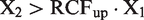
Similarly, a decrease is considered significant when

([X 2 - X 1] / X 1) \cdot 100 < - RCV = > X 2 < (1 - RCV / 100) \cdot X 1

where (1–RCV/100) can be regarded as a factor to multiply the first result to provide the downward significant limit for a decrement. This factor is defined as the reference change factor (RCF_down = 1–RCV/100) and is substituted into the relation as

X 2 < RCF down \cdot X 1

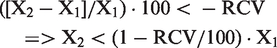
By definitions, RCF_up = 1 + RCV/100 and RCF_down = 1–RCV/100. By substitution of RCV into the relations, the following relation is derived

RCF down = 2 - RCF up

The latter relationship states that, when the RCF_up factor is calculated, then the corresponding RCF_down factor is easily derived for normally distributed data.

Normal distributions of data from simulated healthy individuals were generated with a mean (μ) plus a random number (random) from a normal distribution (with mean = 0 and standard deviation = 1) multiplied by the CV_T and μ. According to Bliss,⁹ this is mathematically expressed as

individualresult = μ + random \cdot CV T / 100 \cdot μ

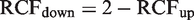
A total of 10,000 simulated healthy normally distributed results were generated for each investigated CV_T (10.0, 20.0, 30.0 and 40.0%). The database of results consisted of 100 columns and 100 rows. From each column, two results were selected as representing serial results from an individual. From one column, sets of two results were selected for testing; i.e. 99 sets consisting of two results from each column were tested. In total, from 100 columns, 9900 individual sets of paired serial results were tested. For each test, it was recorded if X₂ was increased significantly as compared to X₁. Since all the normal distributed data sets were regarded as results from 9900 healthy individuals, the significant increases of X₂ could be recorded as false-positive increases. The RCF_up factor was then determined when 5% of the 9900 tested sets were recorded as having a significant increase for a unidirectional probability of 95% (or the same as when 5% of the X₂ results exceeded the upper significant limit given by the determined RCF_up factor), i.e. when

X 2 (false positiveresults (5 %)) > uppersignificantlimit = RCF up \cdot X 1

In the same way, the RCF_up factor was determined when 1% false-positive results were recorded as having a significant increase for a unidirectional probability of 99%.

Three and more serial results, normal distributions

The difference between three consecutive results, X₁, X₂ and X₃, are considered significant when at least one of the two results (X₂ or X₃) exceed the upper significant limit (RCF_up · X₁); i.e.

If X 2 > RCF up \cdot X 1 or X 3 > RCF up \cdot X 1

Similarly, as for the procedure for two serial results, sets consisting of three results were selected for testing. From one column, sets of three results were selected for RCV testing when three serial results were examined; i.e. 98 sets consisting of three results from each column were tested as serial results from 98 individuals. In total, 9800 individual sets of three serial results were tested. For each test, it was recorded if X₂ or X₃ had a significant increase as compared to X₁. If X₂ or X₃ showed a significant increase, the tested set was recorded as having a significant increase. The RCF_up factor was then determined when the provided upper significant limit recorded 5% and 1% of the 9800 test sets as having significant increases. Similarly, RCF_up factors were calculated for four serial results and then up to 20 serial result sets consisting of 2, 3, 4, 5, 6, 7, 8, 9, 10, 15 and 20 serial results were tested. In total, 99,500 sets of serial results were tested for each CV_T and including four different percentages of CV_T (10.0, 20.0, 30.0 and 40.0%) consequently 398,000 sets (from 398,000 individuals) of serial results were tested. All RCF_up factors were calculated for the significant upper limits of a constant unidirectional probability of 95% (P < 0.05) and 99% (P < 0.01).

Log-normal distributions

Data follow a log-normal distribution if the logarithms follow a normal distribution. The normal distribution is generated as: individual results = μ + random · CV_T/100 · μ. Taking the exponential function of this normal distribution will give an ln-normal distribution. This is mathematically expressed as

individualresult = exp (μ + random \cdot CV T / 100 \cdot μ)

CV_T/100 · μ = standard deviation (σ) which is the standard deviation of the underlying normal distribution. σ is substituted into the relation and is then expressed as

individualresult = exp (μ + random \cdot σ)

Fokkema et al.⁴ have described the relation between σ and CV_T

σ = (ln [(CV T / 100) 2 + 1]) 1 / 2

and we used this for ln-normal calculations for different percentages of CV_T (10.0, 20.0, 30.0, 40.0%) for two and up to 20 serial results. As for normal distributions, RCV_up factors were calculated based on 10,000 of ln-normal distributed results. The number of tested sets of results was the same as for normal distributions. As for normal distributions, the RCF_up factors were calculated to give upper significant limits for a constant unidirectional probability of 95% and 99%, respectively.

Fokkema et al.⁴ have also described the following formulae

RCF_up = exp(Z · 2^½· σ) and RCF_down = exp(–Z · 2^½· σ) and the following is derived from these relationships

RCF up = 1 / RCF down, and RCF down = 1 / RCF up .

As for normal distributions, when RCF_up has been calculated, the corresponding RCF_down is easily derived. Z_n-score calculations were based on ln-normal simulated data. The formula RCF_up = exp(Z_n·2^½·σ) was then rearranged to: Z_n = ln(RCF_up)/(2^½ · σ) in order to calculate the Z_n-scores.

Results

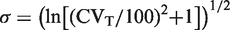
The factors for calculating the upper significance limit, RCF_up, are listed in Table 1 with variables (CV_T, number of results, unidirectional probability of 95% and 99%) for normal distributed and ln-normal distributed simulated data.

Table 1.

RCF_up factors for calculating the upper limits for a significant increase at a constant cumulated unidirectional probability of 95% and 99%.

Number of results^a	RCF_up (95% probability)
	CV_T = 10.0%		CV_T = 20.0%		CV_T = 30.0%		CV_T = 40.0%
	Normal^b	Ln-normal^c	Normal^b	Ln-normal^c	Normal^b	Ln-normal^c	Normal^b	Ln-normal^c
2	1.26	1.26	1.62	1.58	2.16	1.98	3.16	2.44
3	1.31	1.31	1.75	1.71	2.44	2.22	3.76	2.84
4	1.34	1.34	1.82	1.78	2.61	2.35	4.14	3.07
5	1.35	1.36	1.87	1.83	2.68	2.44	4.36	3.23
6	1.37	1.37	1.90	1.87	2.78	2.53	4.57	3.37
7	1.38	1.38	1.93	1.90	2.83	2.60	4.68	3.50
8	1.39	1.39	1.96	1.92	2.86	2.63	4.77	3.56
9	1.40	1.40	1.97	1.94	2.91	2.68	4.80	3.64
10	1.40	1.41	1.98	1.97	2.95	2.73	4.87	3.74
15	1.43	1.44	2.04	2.05	3.08	2.90	5.10	4.05
20	1.44	1.46	2.09	2.10	3.14	3.01	5.29	4.24
	RCF_up (99% probability)
2	1.39	1.38	2.05	1.90	3.52	2.59	13.0	3.49
3	1.45	1.44	2.20	2.05	3.91	2.89	14.1	4.03
4	1.47	1.46	2.28	2.11	4.09	3.03	16.3	4.29
5	1.49	1.48	2.36	2.19	4.41	3.19	20.2	4.58
6	1.52	1.50	2.41	2.24	4.55	3.30	20.3	4.80
7	1.52	1.51	2.43	2.27	4.77	3.37	20.3	4.92
8	1.52	1.52	2.45	2.30	4.85	3.42	21.2	5.02
9	1.53	1.53	2.46	2.32	4.89	3.47	21.2	5.12
10	1.54	1.53	2.48	2.33	4.90	3.49	21.3	5.16
15	1.56	1.55	2.55	2.39	5.03	3.65	22.5	5.47
20	1.58	1.59	2.61	2.49	5.22	3.86	25.1	5.87

RCF_up: factor to multiply the first result when calculating the upper limit for a significant increase in concentrations; CV_T: total coefficient of variation.

Simulated concentration data from healthy individuals.

Data based on normal (Gaussian) distributions.

Data based on ln-normal (ln-Gaussian) distributions.

Normal distributions

Normal data distributions are symmetrical around the mean. The generated simulated data sets showed that more results were extremely low (near zero) or even negative when CV_T increased. According to the practical use of the traditional RCV calculations, the change between two results is related to the first result (see Methods). If the first result (X₁) is low or zero, the second result (X₂) will be recorded as a significant increase. Therefore, also very small increments will be recorded as significant. Consequently, the RCF_up factors calculated in Table 1 based on simulated data sets are greater than the theoretically RCF_up calculations (based on [RCF_up = 1 + RCV/100]). For example, for two serial results and use of a unidirectional probability of 95% (Z = 1.65), the RCF_up results based on the theoretically RCF_up calculations were 1.23; 1.47; 1.70 and 1.93 for CV_T (10.0, 20.0, 30.0 and 40.0%), respectively; and the corresponding RCF_up results based on the simulations (Table 1) were 1.26; 1.62; 2.16 and 3.16. Obviously, these differences increase as CV_T increases. For CV_T = 40% and 99% probability, the RCF_up factors were extremely high (RCF_up > 13, Table 1).

Ln-normal distributions

The results for RCF_up factors listed in Table 1, for two measurements and based on simulated ln-normally distributed data, are approximately the same as calculated from the formula: RCF_up = exp(Z · 2^½· σ).⁴ In Table 2, the Z_n-scores are calculated for different percentages of CV_T and number of results (n). For two results, the Z₂-scores for 95% and 99% probability are approximately constant and indistinguishable from the Z-scores 1.65 and 2.33 used in the formula: (RCF_up = exp[Z · 2^½· σ]). Similarly, the Z_n-scores are calculated for three and up to 20 results and these Z_n-scores remain also approximately constant. Thus, the formula is also valid for more than two serial results with Z_n-scores increasing with number of results. This increase in Z_n-scores reflects the cumulated significance of more false-positive results with more tests (Table 2). Also, the results for RCF_down factors calculated based on simulation data are the same as calculated from the formula: RCF_down = exp(−Z · 2^½· σ).⁴ Furthermore, the relationship σ = (ln[(CV_T/100)²+ 1])^½ was confirmed in CV_T calculations of all the ln-normal data (data not shown). From the same relationship, it can be shown that σ ∼ CV_T; i.e. σ and CV_T are approximately the same up to about CV_T = 30%. Therefore, in practice, the following relation is useful for RCF_up calculations for CV_T < 30% and relevant number of results, n

RCF up = exp (Z n \cdot 2 1 / 2 \cdot CV T / 100)

Table 2.

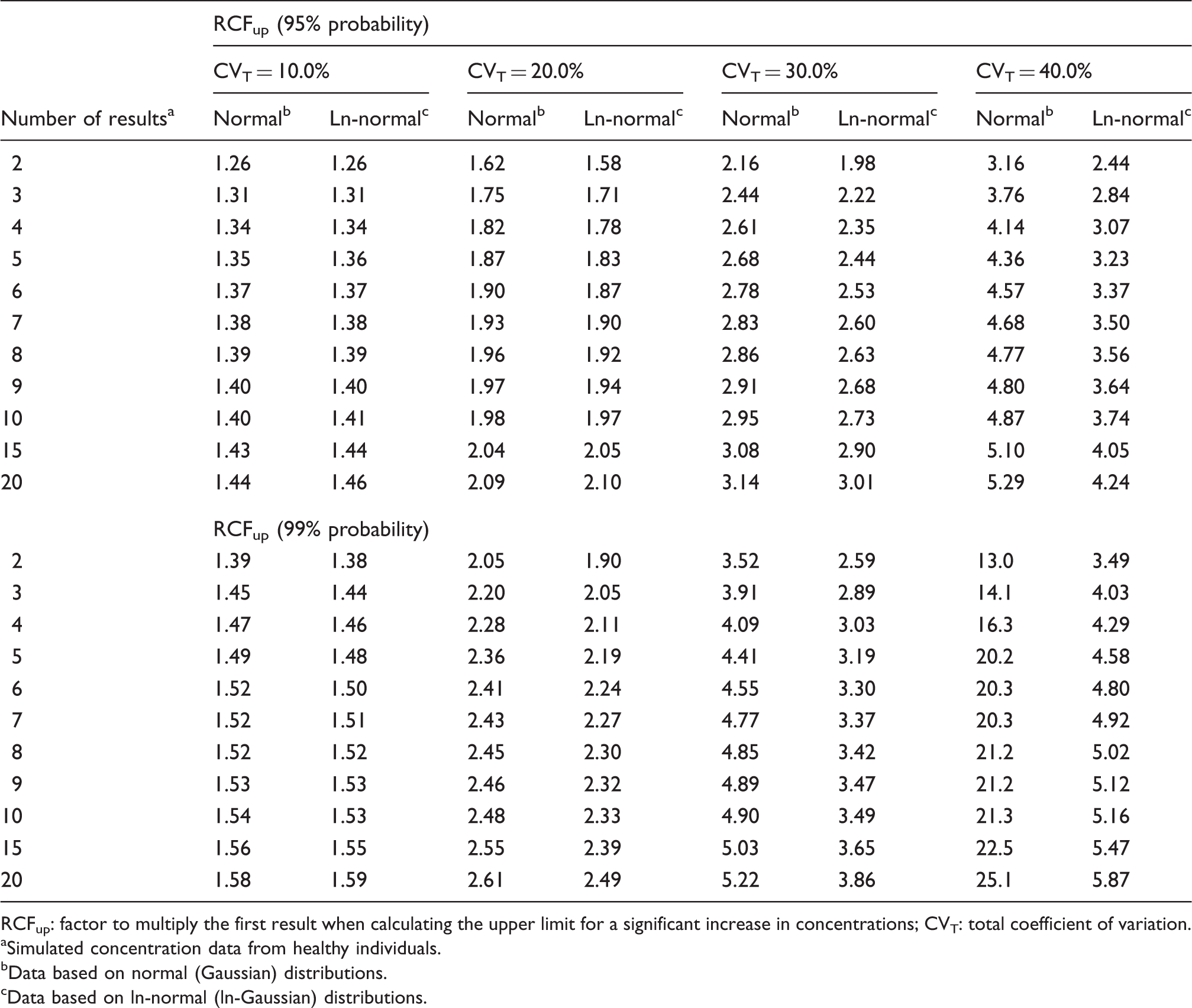
Z_n-scores^a dependent on the number of serial results (n).

Number of results (n)	Z_n-scores^a (95% probability)
Number of results (n)	CV_T= 10.0%	CV_T= 20.0%	CV_T= 30.0%	CV_T= 40.0%
2	1.64^b	1.63^b	1.65^b	1.64^b
3	1.91	1.92	1.92	1.92
4	2.07	2.06	2.06	2.06
5	2.18	2.16	2.15	2.15
6	2.23	2.24	2.24	2.23
7	2.28	2.29	2.30	2.30
8	2.33	2.33	2.33	2.33
9	2.38	2.37	2.38	2.37
10	2.43	2.42	2.42	2.42
15	2.58	2.56	2.57	2.57
20	2.68	2.65	2.65	2.65
	Z_n-scores^a (99% probability)
2	2.28^c	2.29^c	2.29^c	2.29^c
3	2.58	2.56	2.56	2.56
4	2.68	2.67	2.67	2.67
5	2.78	2.80	2.79	2.79
6	2.87	2.88	2.88	2.88
7	2.92	2.93	2.93	2.92
8	2.97	2.97	2.96	2.96
9	3.01	3.01	3.00	3.00
10	3.01	3.02	3.01	3.01
15	3.11	3.11	3.12	3.12
20	3.29	3.26	3.25	3.25

Z_n-scores were used to calculate RCF_up factors for unidirectional changes during serial monitoring. Z_n-scores were calculated using the formula Z_n = ln(RCF_up)/(2½ • σ). RCF_up results are used from Table 1 giving a constant cumulated unidirectional probability of 95%, and 99% and are based on ln-normal distributions from healthy individuals. σ = (ln[(CV_T/100)²+ 1])^½ and is calculated based on different CV_T^. CV_T, denotes total coefficient of variation.

Z₂ results estimated from simulations should be equal to Z = 1.65 used for traditional RCV.

Z₂ results estimated from simulations should be equal to Z = 2.33 used for traditional RCV.

Discussion

General considerations

With the introduction of the concept of RCV, in 1983,¹ an excellent tool for interpretation of consecutive unidirectional measurements in patients became available and today practically all articles about the application of data on biological variation include calculations of RCV. Originally, Harris and Yasaka¹ used standard deviations for the calculations but following numerous publications showing rather constant coefficients of CV_I, the consequence was that the RCV most often became based on CV_T.² Within the last decade, discussions about normal and ln-normal distributions of biological parameters have become intense and the tendency is now moving towards the application of ln-distributions.^4–8 One problem with the RCV is that it can only be used in assessment of differences between two serial results, which makes it susceptible to the effect of repeated testing, where the probability of false-positive results increases with the number of results available. Therefore, a new concept to overcome the problems with repeated testing, by keeping the probability of false-positive results constant for several consecutive results and only dependent on the number of results available seems worthwhile.

The new model

In the new model, we have solved the problem of repeated testing by expanding the actual test value, denoted Z_n, in relationship to the number of results available in the monitoring sequence. Thereby, the cumulated probability of false-positive results, either 5% or 1%, is kept constant for the individual during the whole monitoring period. These Z_n scores are independent of CV_T and make it easy to calculate the limit for each new result according to the chosen total cumulated level of unidirectional significance for the individual. Furthermore, we have investigated the influence of normally distributed individual data and found that practical use of the traditional RCV method to test a difference through assessment of the difference from the first measurement is susceptible to low concentration values for the first result. This is not a problem for the ln-normally distributed data (Table 1). We have shown that the practical use of traditional RCV calculations will produce too many false-positive results, especially for high values of CV_T, compared to theoretical RCV calculations. On the other hand, the calculated RCF_up factors are comparable for both normal and ln-normal distributions up to about CV_T = 20.0% (Table 1). At higher CV_T, the RCF_up factor results for normal distributions will exceed the RCF_up factors for ln-normal distributions and, in addition, the RCF_up factors will also be greater than 2 (Table 1). From the relation RCF_down = 2–RCF_up, it is also obvious that RCF_down will be negative for RCF_up >2 and make no sense, since the significant limit for decreasing results will be negative for normal distributions. Consequently, we recommend that all calculations of limits for unidirectional significant differences should be based on ln-normal distributions, i.e. RCF_up = exp(Z_n · 2^½ · CV_T/100). Compared with traditional RCV calculation (RCV = [Z · 2^½ · CV_T]), the proposed significance calculations based on ln-normal distributions may seem more complicated. However, the only difference in variables compared with traditional RCV calculations is the Z_n-score obtained from Table 2 for more than two serial results. It should be noticed, that the Z_n-scores are dependent on the number of serial results (n) and probability level – but are independent of CV_T. In contrast to traditional RCV calculations, an additional merit of use of RCF factors is that the significant limits are given as simple numbers with appropriate units. For the sake of clarity and space, we have focused on unidirectional differences. However, the RCV, RCF_up, RCF_down and Z_n calculations could also be applied to bidirectional differences. A bidirectional change is used when both increases and decreases of results are being considered. This aspect will be addressed in another communication.

Simulation models have also been used in several monitoring studies to validate the utility of different criteria to interpret increments in serial cancer biomarker concentrations.^10–12 In addition, this model system may also be suitable for Phase I development of new cancer biomarker assessment and to optimize already existing criteria.¹³

An example of calculation of limits for significant unidirectional differences for up to six serial results

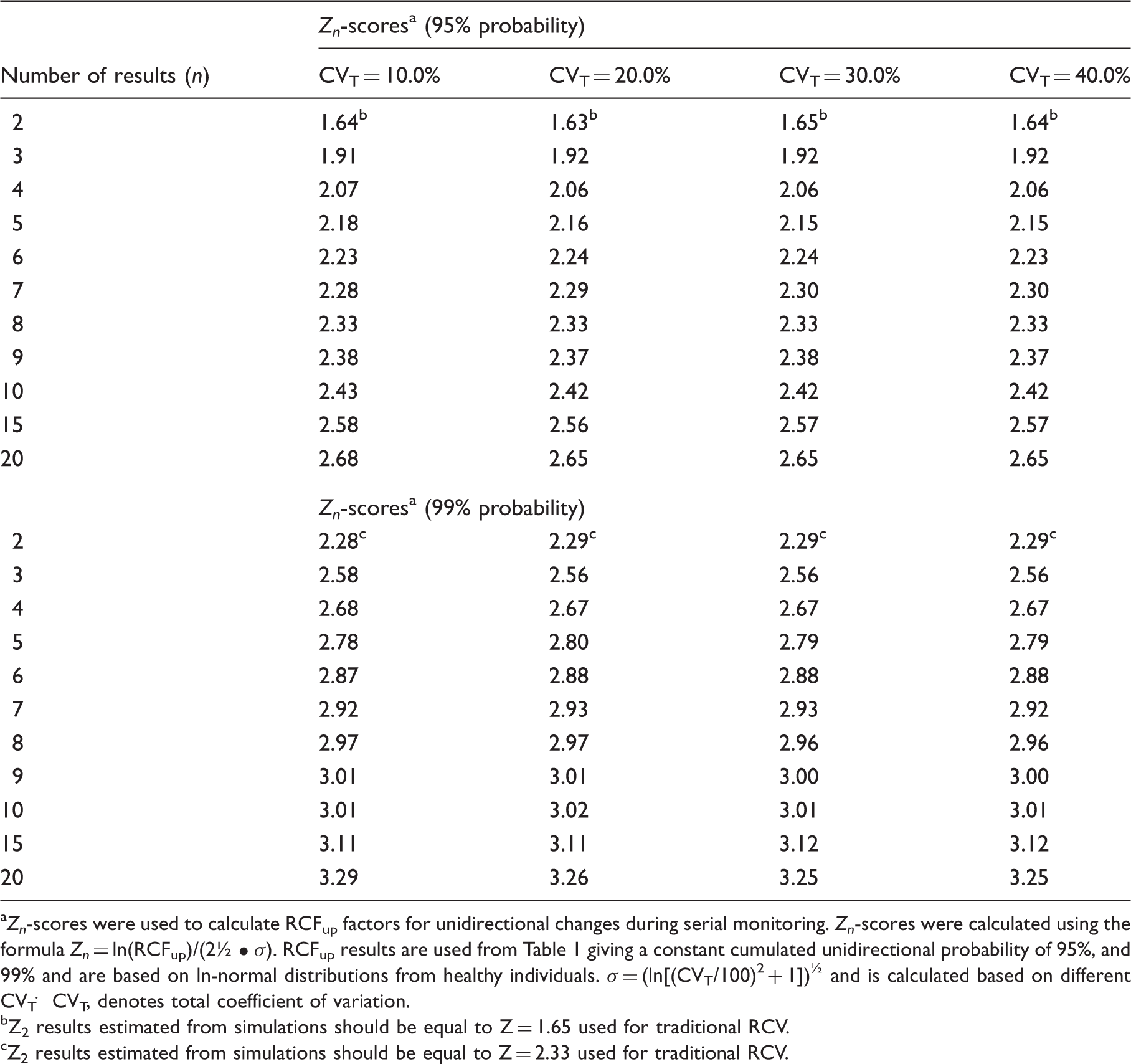
As an example, Fraser³ has described a case of changes in liver function tests in a 63-year-old man who was prescribed statin therapy to lower his less-than-ideal serum cholesterol concentration. The serum aspartate aminotransferase (AST) concentration rose with time (16, 18, 24, 40, 54, 69 U/L). 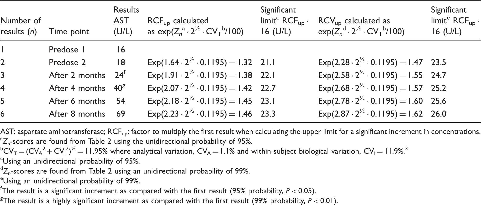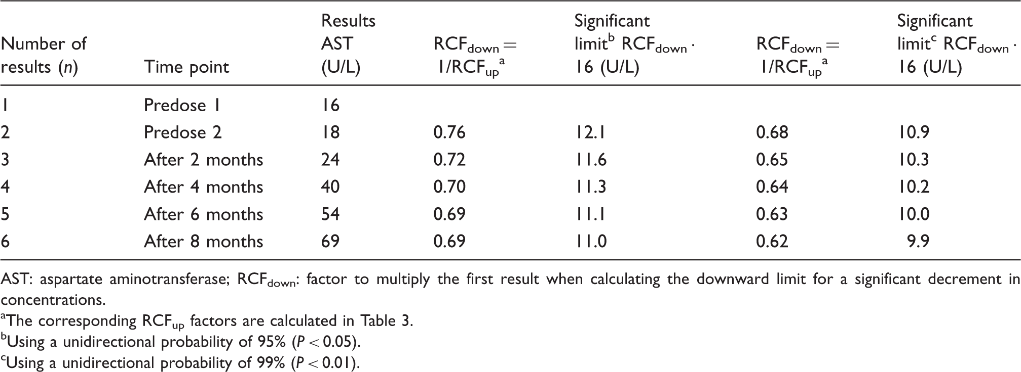The results of the serum AST activities from the patient treated with statin are used for the calculations.³ The method is also presented in Table 3 and (RCF_up = exp[Z_n · 2^½ · CV_T/100]) is used for the calculations. The limits for both significant (P < 0.05) and highly significant (P < 0.01) increments are calculated (RCF_up factor multiplied by first result) and listed with the serial results in Table 3. These results are also illustrated in Figure 1. From both Table 3 and Figure 1, it is clearly shown that, when the increments in serial concentrations exceed the significant limit (result 3) and the highly significant limit (result 4). Note that, as a consequence of the developed method, the concentration limits increase with the number of results due to the constant cumulated percentage of false positives during repeated testing. For application of the complete method, the downward significant limits are also calculated and listed in Table 4 – although not relevant for the actual example.

Figure 1.

Serum aspartate aminotransferase concentrations in a patient treated with statin. The significant upper limits for increments were calculated using unidirectional probabilities of 95% and 99%.

Table 3.

Calculation of upper limits for significant increments in serum AST concentrations in a patient treated with statin.³

Number of results (n)	Time point	Results AST (U/L)	RCF_up calculated as exp(Z_n^a · 2^½ · CV_T^b/100)	Significant limit^c RCF_up · 16 (U/L)	RCV_up calculated as exp(Z_n^d · 2^½ · CV_T^b/100)	Significant limit^e RCF_up · 16 (U/L)
1	Predose 1	16
2	Predose 2	18	Exp(1.64 · 2^½ · 0.1195) = 1.32	21.1	Exp(2.28 · 2^½ · 0.1195) = 1.47	23.5
3	After 2 months	24^f	Exp(1.91 · 2^½ · 0.1195) = 1.38	22.1	Exp(2.58 · 2^½ · 0.1195) = 1.55	24.7
4	After 4 months	40^g	Exp(2.07 · 2^½ · 0.1195) = 1.42	22.7	Exp(2.68 · 2^½ · 0.1195) = 1.57	25.2
5	After 6 months	54	Exp(2.18 · 2^½ · 0.1195) = 1.45	23.1	Exp(2.78 · 2^½ · 0.1195) = 1.60	25.6
6	After 8 months	69	Exp(2.23 · 2^½ · 0.1195) = 1.46	23.3	Exp(2.87 · 2^½ · 0.1195) = 1.62	26.0

AST: aspartate aminotransferase; RCF_up: factor to multiply the first result when calculating the upper limit for a significant increment in concentrations.

Z_n-scores are found from Table 2 using the unidirectional probability of 95%.

CV_T = (CV_A²+ CV_I²)^½= 11.95% where analytical variation, CV_A = 1.1% and within-subject biological variation, CV_I = 11.9%.³

Using an unidirectional probability of 95%.

Z_n-scores are found from Table 2 using an unidirectional probability of 99%.

Using an unidirectional probability of 99%.

The result is a significant increment as compared with the first result (95% probability, P < 0.05).

The result is a highly significant increment as compared with the first result (99% probability, P < 0.01).

Table 4.

Calculation of downward limits for significant decrements in serum AST concentrations in a patient treated with statin.³

Number of results (n)	Time point	Results AST (U/L)	RCF_down = 1/RCF_up^a	Significant limit^b RCF_down · 16 (U/L)	RCF_down = 1/RCF_up^a	Significant limit^c RCF_down · 16 (U/L)
1	Predose 1	16
2	Predose 2	18	0.76	12.1	0.68	10.9
3	After 2 months	24	0.72	11.6	0.65	10.3
4	After 4 months	40	0.70	11.3	0.64	10.2
5	After 6 months	54	0.69	11.1	0.63	10.0
6	After 8 months	69	0.69	11.0	0.62	9.9

AST: aspartate aminotransferase; RCF_down: factor to multiply the first result when calculating the downward limit for a significant decrement in concentrations.

The corresponding RCF_up factors are calculated in Table 3.

Using a unidirectional probability of 95% (P < 0.05).

Using a unidirectional probability of 99% (P < 0.01).

Conclusions

A simple calculation of limits for significant unidirectional differences in two or more results of a biomarker. The upper limit for significant increment of serial results is calculated by a factor RCF_up. If X₁ is the first result, then upper limit is found with X₁ multiplied by RCF_up

upperlimit = X 1 \cdot RCF up

The RCF_up factor is calculated from the relationship

RCF up = exp (Z n \cdot 2 1 / 2 \cdot CV T / 100)

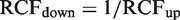
The Z_n is found from Table 2 and CV_T is calculated using estimates of CV_A and CV_I (CV_T = [CV_A²+ CV_I²]^½). The corresponding downward limit for a significant decrement of serial results is calculated by a factor RCF_down (downward limit = X₁ · RCF_down). RCF_down factor is found from the relationship

RCF down = 1 / RCF up

Footnotes

Acknowledgements

The authors would like to thank Merete Frejstrup Pedersen for her assistance in generating the figure.

Declaration of conflicting interests

None.

Funding

This research received no specific grant from any funding agency in the public, commercial, or not-for-profit sectors.

Ethical approval

Not required.

Guarantor

FL.

Contributorship

FL and PHP designed and generated the computer simulations. FL wrote the first draft of the manuscript. All authors contributed to the discussions, and reviewed and edited the manuscript.

References

Harris

Yasaka

. On the calculation of a “reference change” for comparing two consecutive measurements. Clin Chem 1983; 29: 25–30.

Ricós

Garcia-Lario

Alvares

. Biological variation database on biological variation: pros, cons and progress. Scand J Clin Lab Invest 1999; 59: 491–500.

Fraser

. Biological variation: from principles to practice, Washington, DC: AACC Press, 2001.

Fokkema

Hermann

Muskiet

FAJ

. Reference change values for brain natriuretic peptides revisited. Clin Chem 2006; 52: 1602–1603.

Klersy

d'Ezril

GVM

Barassi

. Advantages of the lognormal approach to determining reference change values for N-terminal propeptide B-type batriuretic peptide. Clin Chim Act 2012; 413: 544–547.

Møller

Hyltoft Petersen

Rejnmark

. Biological variation of soluble CD163. Scand J Clin Lab Invest 2003; 63: 15–22.

Tuxen

Sölétormos

Hyltoft Petersen

. Interpretation of sequential measurements of cancer antigen 125 (CA 125), carcinoembryonic antigen (CEA), and tissue polypeptide antigen (TPA) based on analytical imprecision and biological variation in the monitoring of ovarian cancer. Clin Chem Lab Med 2001; 39: 531–538.

Limpert

Stahel

Abbt

. Log-normal distribution across the sciences: keys and clues. BioScience 2001; 51: 341–352.

Bliss

. Statistics in biology, New York: McGraw-Hill Book Company, 1967.

10.

Sölétormos

Hyltoft Petersen

Dombernowsky

. Progression criteria for cancer antigen 15.3 and carcinoembryonic antigen in metastatic breast cancer compared by computer simulation of marker data. Clin Chem 2000; 46: 939–949.

11.

Petersen

Sölétormos

Pedersen

. Interpretation of increments in serial tumour biomarker concentrations depends on the distance of the baseline concentration from the cut-off. Clin Chem Lab Med 2011; 49: 303–310.

12.

Lund

Hyltoft Petersen

Pedersen

. Criteria to interpret cancer biomarker increments crossing the recommended cut-off compared in a simulation model focusing on false positive signals and tumour detection time. Clin Chim Act 2014; 431: 192–197.

13.

Sölétormos

Duffy

Hayes

. Design of tumor biomarker-monitoring trials: a proposal by the European Group on Tumor Markers. Clin Chem 2013; 59: 52–59.

Calculation of limits for significant unidirectional changes in two or more serial results of a biomarker based on a computer simulation model

Abstract

Background

Methods

Results

Conclusions

Keywords

Introduction

Materials and methods

Two serial results, normal distributions

Three and more serial results, normal distributions

Log-normal distributions

Results

Normal distributions

Ln-normal distributions

Discussion

General considerations

The new model

An example of calculation of limits for significant unidirectional differences for up to six serial results

Conclusions

Footnotes

Acknowledgements

Declaration of conflicting interests

Funding

Ethical approval

Guarantor

Contributorship

References