A dynamic reference change value model applied to ongoing assessment of the steady state of a biomarker using more than two serial results

Abstract

Background

Reference change values are used to assess the significance of a difference in two consecutive results from an individual. Reference change value calculations provide the limits for significant differences between two results due to analytical and inherent biological variations. Often more than two serial results are available. Using the reference change value concept on more than two measurements results in an increased number of false-positive results. This problem has been solved for both uni- and bidirectional differences through use of wider limits when additional results are included.

Methods

Based on normally (Gaussianly) distributed simulated data, a dynamic reference change value model was developed using more than two results and total coefficients of variation. The dynamic reference change value model includes validation of a set-point as the mean of the four first serial results and additional results are assessed for compliance to the steady state with the same set-point. Furthermore, the dynamic reference change value model compensates for increasing false-positive results with subsequent results. The dynamic reference change value model was designed to calculate significant limits for bidirectional differences.

Results

Reference change factors were calculated for multiplication of the mean of previous results to create the limits for significant differences. The reference change factors are provided as a function of number of results and total coefficients of variation both in tables and in figures.

Conclusions

The dynamic reference change value model is appropriate for ongoing assessment of the steady state of a biomarker using more than two serial results.

Introduction

Reference change values (RCV) are used to assist with the objective assessment of differences in the results of two consecutive measurements of a biomarker from an individual. RCV calculations provide the limits for differences in two results due to analytical variation and inherent within-subject biological variation, i.e. if a measured difference is greater than the theoretical RCV limits, it is considered significant. Harris and Yasaka ¹ first described the application of RCV in which, for two results, X1 and X2, the RCV limits for a change in concentration are RCV = ± Z · 2^½ · SD_T, where SD_T is the total standard deviation (SD) of analytical (SD_A) plus within-subject biological variation (SD_I), [SD_T = (SD_A² + SD_I²)^½]. Z is the number of SD appropriate to the probability desired for detecting whether a difference has occurred: this was documented as a two-sided (bidirectional) application. However, in practice, data on within-subject biological variation for most measurands are given as coefficients of variation (CVs). Therefore, the most commonly cited and applied formula for calculating RCV limits is RCV = ± Z · 2^½ · (CV_A² + CV_I²)^½, where CV_A is the analytical coefficient of variation and CV_I is the within-subject biological variation. Often the formula is given as RCV = ±Z · 2^½ · CV_T, where CV_T, as above, is the total CV, CV_T = (CV_A² + CV_I²)^½. Nevertheless, when using this usual, or what we have termed ‘common’, RCV formula with CV_T, the calculated symmetric limits will be incorrect due to the ‘skew’ measured difference (X2−X1)/X1, where X1 and X2 are the found results. Recently, it has been shown that this ‘common’ RCV method will give up to 9.32% false-positive results as compared with the theoretical 5.0% false-positive results for increasing concentrations (when CV_T = 20% and using unidirectional differences at P < 0.05 with Z = 1.65). ²

The ‘common’ RCV calculation is based on only two consecutive results, but in practice, often more than two serial results from an individual are available. However, if further simple RCV calculations are used in sequence, the probability will change, so every time an individual is re-tested (repeated testing), the number of false-positive results will increase. Using simulation studies concerning serial testing, this problem has been solved for both uni- and bidirectional changes by use of wider limits when additional results are included.^3,4 In the model of Lund et al.,^3,4 the RCV limits were performed wider with use of Z_n score dependent of number (n) of serial results based on simulations. Following this, Liu et al. ⁵ introduced a mathematical formula to calculate the same Z_n scores. In consequence: the ability to detect minor changes in results will be reduced. Jones and Chung ⁶ introduced an alternative RCV concept for serial results in which the limits will become narrower when further results are included. Assumptions in this model require that the results should follow a normal (Gaussian) distribution in steady state both before and after a possible clinical event. Moreover, this concept uses the mean from all results before a clinical event as an estimate of a homeostatic set-point and, similarly, uses the mean of results after the event as an estimate of a (possibly) new set-point. However, these RCV calculations are only valid when SD is used and the assumptions used in their model have not been subjected to objective examination. ⁷ Subsequently, these authors concluded ‘that developing appropriate calculations for RCV is indeed a difficult task’ when using more than two results and total variations are given as CV_T. ⁸ The concept of using the mean of further results for estimating a set-point is an excellent idea if steady state conditions can be confirmed, but Jones and Chung ⁸ did not provide an answer to their stated difficulty.

A potential method to overcome the difficulty could be to test the steady state condition for each additional result in a continuous process up to, for example, four results and calculating the mean to be subsequently used as the set-point for assessment of whether further results are different. Then, the variation around this set-point is reduced by half and, thus, the ability to detect smaller significant differences in serial results from an individual will increase substantially. ⁶

The aim of this project was to develop a dynamic RCV (d-RCV) model using more than two serial results and total variations given as CV_T. Firstly, an estimate of a homeostatic set-point as a mean of four serial results is validated. Secondly, if a set-point is determined, then additional serial results are tested to assess whether they are in steady state with the same set-point. Thirdly, the d-RCV calculations should be compensated for increasing false-positive results due to the repeated testing. Finally, the d-RCV model is compared with other RCV concepts and the influence of repeated testing on the RCV calculations is documented.

Materials and methods

All data for the simulations were generated using Microsoft Excel version 2010. The fundamental basis for the model is the use of repeated testing of an individual, i.e. every time a new result is obtained, it is compared with previous results.

Simulations

The simulation methods have been described in detail in previous publications.^3,4 Briefly, the d-RCF calculations were based on normally (Gaussianly) distributed simulated data. Based on the d-RCV model, bidirectional changes were considered, i.e. both increases and decrease in results were calculated. ⁴ The Z value was chosen as Z = 1.96, i.e. 2.5% false-positive results > upper significant limit plus 2.5% false-positive results < downward limit. The simulations were generated with use of repeated testing; i.e., every time a new result is compared with previous results, the number of false-positive results is cumulated and kept constant (as ± 2.5%) after every simulation.

d-RCV model – Validation of a homeostatic set-point for increases (also described in Figure 1)

All d-RCF (Up and Down) values were calculated using simulations.

N is the number of serial results.

N = 2

Given two consecutive results, X1 and X2, X1 (=mean₁) is regarded as an estimate of the set-point. d-RCF_up is the factor used to multiply the first result to provide the upper significant limit for a rise (Table 1). If X2 > X1, i.e. an increase in results has occurred and, if

$$\text{X2}>\text{d}\text{-}{\text{RCF}}_{\text{up2}}\cdot {\text{mean}}_{\text{1}}$$

the increase is significant and this set-point (X1= mean₁) is not accepted as the set-point. However, X2 could be an estimate of a new set-point and the test procedure could start again. In contrast, if

$$\text{X2}<\text{d}-{\text{RCF}}_{\text{up2}}\cdot {\text{mean}}_1$$

then the increase is actually within the limit for variation of CV_T and a new (and better) estimate of the set-point is indicated as a mean of the two results, i.e. mean₂ = (X1 + X2)/2. Similarly, the further calculation procedures with additional results (X3, X4 etc.) are shown in Figure 1 using the d-RCF_up factors (d-RCF_up2 to d-RCF_up11) from Table 1.

Figure 1.

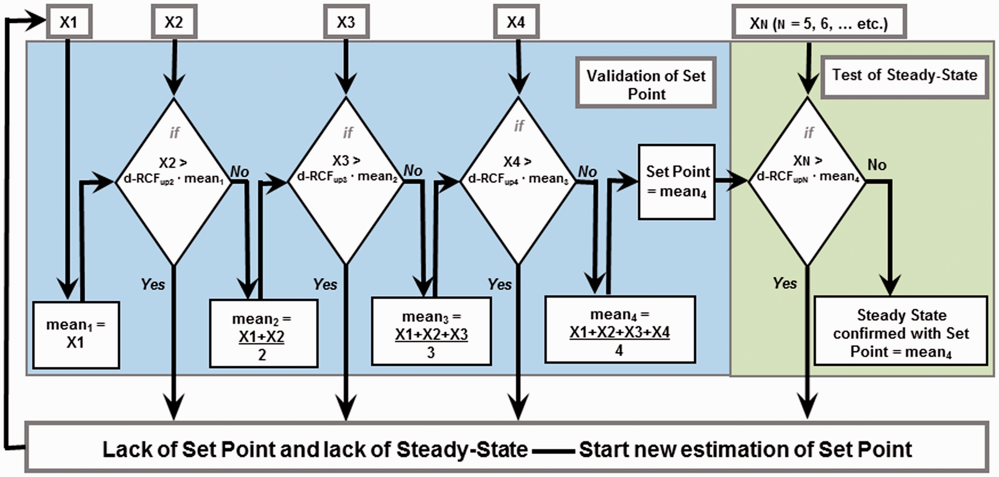
The dynamic RCV (d-RCV) model used to calculate limits of a biomarker to assess steady state. Given is increasing X serial results and validation of a homeostatic set-point: Given is two consecutive results, X1 and X2. First result X1 is mean₁ and an increase X2 is compared with d-RCF_up2 · mean₁. If X2 > d-RCF_up2 · mean₁, the increase is significant and the individual has no set-point and is not in steady state. X2 could then be an estimate of a set-point and a new assessment could be started. In contrast, if X2 < d-RCF_up2· mean₁, the increase is not significant and mean of X1 and X2 is an estimate of a possible set-point. Given then the third result X3, which is compared with d-RCF_up3 · mean₂, and the similar procedure is repeated as with two results until the fourth result X4 and if differences between all these results are not significant, a set-point is determined as mean₄. Assessment of steady state for further results XN (N = 5, 6, …etc.) in a similar procedure is assessed as being in steady state with use of mean₄ and the associated d-RCF_up value. The d-RCF_up values are provided in Table 1.

Table 1.

Simulated calculations of d-RCF_up (up for increase) and d-RCF_down (down for decrease) for bi-directional changes; CV_T is from 1.0% to 20.0%, Z = 1.96 with use of repeated testing applied in the d-RCV model based on normal (Gauss) distributed simulated results.

CVT%	d-RCF	N=2	N=3	N=4	N=5	N=6	N=7	N=8	N=9	N=10	N=11
1	Up	1.028	1.030	1.031	1.032	1.032	1.032	1.033	1.033	1.033	1.034
	Down	0.9726	0.9706	0.9697	0.9692	0.9687	0.9683	0.9679	0.9676	0.9673	0.9671
2	Up	1.057	1.061	1.063	1.064	1.065	1.065	1.066	1.067	1.067	1.068
	Down	0.9459	0.9419	0.9401	0.9390	0.9381	0.9374	0.9364	0.9358	0.9353	0.9348
3	Up	1.087	1.093	1.095	1.097	1.098	1.099	1.100	1.101	1.102	1.103
	Down	0.9200	0.9140	0.9112	0.9095	0.9081	0.9068	0.9056	0.9047	0.9039	0.9031
4	Up	1.117	1.126	1.129	1.131	1.133	1.134	1.135	1.136	1.137	1.139
	Down	0.8945	0.8867	0.8830	0.8805	0.8788	0.8770	0.8753	0.8740	0.8728	0.8719
5	Up	1.149	1.160	1.164	1.166	1.168	1.170	1.171	1.173	1.174	1.176
	Down	0.8700	0.8600	0.8553	0.8522	0.8499	0.8477	0.8455	0.8438	0.8424	0.8413
6	Up	1.181	1.195	1.199	1.202	1.205	1.207	1.209	1.210	1.211	1.214
	Down	0.8457	0.8337	0.8280	0.8244	0.8215	0.8190	0.8160	0.8142	0.8125	0.8111
7	Up	1.215	1.231	1.236	1.240	1.242	1.245	1.247	1.248	1.250	1.253
	Down	0.8220	0.8080	0.8016	0.7970	0.7937	0.7905	0.7872	0.7850	0.7830	0.7813
8	Up	1.250	1.268	1.274	1.278	1.281	1.284	1.286	1.288	1.290	1.293
	Down	0.7990	0.7828	0.7755	0.7703	0.7660	0.7625	0.7590	0.7562	0.7593	0.7520
9	Up	1.286	1.307	1.313	1.318	1.321	1.324	1.327	1.329	1.331	1.334
	Down	0.7765	0.7580	0.7497	0.7438	0.7389	0.7350	0.7310	0.7277	0.7251	0.7231
10	Up	1.325	1.3470	1.354	1.359	1.362	1.366	1.368	1.371	1.373	1.377
	Down	0.7543	0.7340	0.7243	0.7180	0.7125	0.7079	0.7035	0.6995	0.6967	0.6942
11	Up	1.363	1.389	1.397	1.401	1.406	1.409	1.412	1.414	1.417	1.421
	Down	0.7324	0.7100	0.6995	0.6922	0.6860	0.6809	0.6764	0.6720	0.6685	0.6656
12	Up	1.404	1.433	1.441	1.446	1.450	1.453	1.457	1.459	1.462	1.467
	Down	0.7110	0.6865	0.6749	0.6667	0.6600	0.6540	0.6493	0.6445	0.6406	0.6372
13	Up	1.446	1.478	1.487	1.492	1.496	1.500	1.503	1.506	1.509	1.514
	Down	0.6900	0.6633	0.6505	0.6417	0.6340	0.6275	0.6219	0.6170	0.6130	0.6094
14	Up	1.490	1.525	1.535	1.540	1.544	1.548	1.552	1.555	1.558	1.564
	Down	0.6695	0.6408	0.6266	0.6169	0.6087	0.6015	0.5950	0.5900	0.5857	0.5820
15	Up	1.537	1.575	1.585	1.590	1.595	1.599	1.603	1.606	1.609	1.614
	Down	0.6492	0.6185	0.6031	0.5922	0.5830	0.5755	0.5686	0.5630	0.5586	0.5545
16	Up	1.587	1.626	1.637	1.643	1.647	1.651	1.655	1.657	1.662	1.668
	Down	0.6294	0.5965	0.5800	0.5679	0.5580	0.5500	0.5425	0.5368	0.5315	0.5272
17	Up	1.638	1.680	1.691	1.697	1.702	1.706	1.710	1.713	1.717	1.723
	Down	0.6100	0.5744	0.5565	0.5438	0.5335	0.5245	0.5165	0.5100	0.5048	0.5001
18	Up	1.692	1.737	1.750	1.755	1.760	1.764	1.766	1.770	1.775	1.781
	Down	0.5905	0.5530	0.5335	0.5198	0.5090	0.4990	0.4910	0.4844	0.4779	0.4730
19	Up	1.748	1.797	1.809	1.815	1.820	1.825	1.828	1.832	1.837	1.843
	Down	0.5710	0.5318	0.5110	0.4959	0.4843	0.4735	0.4650	0.4581	0.4515	0.4461
20	Up	1.811	1.860	1.873	1.878	1.884	1.888	1.893	1.897	1.901	1.909
	Down	0.5521	0.5107	0.4885	0.4722	0.4597	0.4490	0.4395	0.4320	0.4254	0.4193

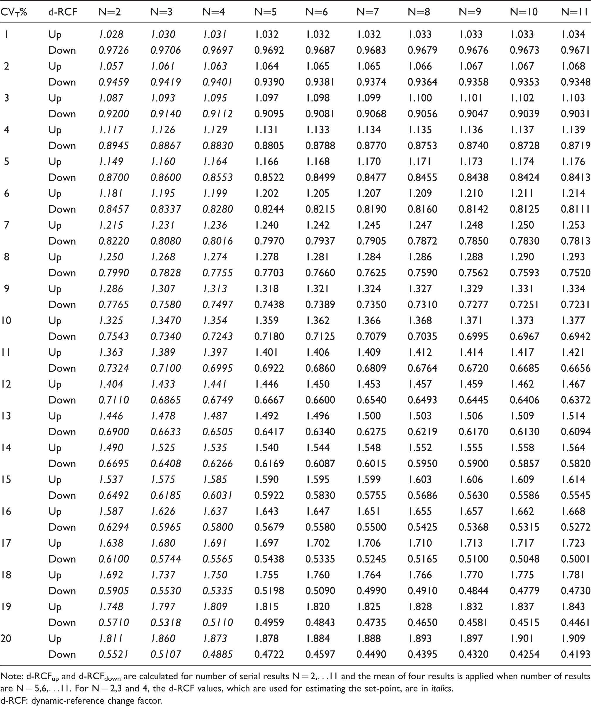
Note: d-RCF_up and d-RCF_down are calculated for number of serial results N = 2,…11 and the mean of four results is applied when number of results are N = 5,6,…11. For N = 2,3 and 4, the d-RCF values, which are used for estimating the set-point, are in italics.

d-RCF: dynamic-reference change factor.

If four results are validated as having no significant increases, a steady state with a set-point is determined as mean₄. Further results (X5, X6, etc.) are all compared with mean₄ in the calculations. If the new results are not significantly different, the steady state is confirmed for each new result. If this new result is a significant increase, the steady state has ended and the new result could be an estimate of a new set-point and the process of objective assessment of whether an increase has occurred can start again.

d-RCV model – Testing of a homeostatic set-point for decreases

Similarly, when the last result is a decrease compared with the mean of previous results (up to mean₄), the analogous d-RCF_down factors (d-RCF_down2 to d-RCF_down11) are used (Table 1).

Conversion from d-RCF to d-RCV%

Figure 2 was generated using the d-RCF results from Table 1 by conversion to d-RCV% as d-RCV% Up and d-RCV% Down using the following two formulae

$$\text{d}-\text{RCV}\%\text{Up}=\left(\text{d}-{\text{RCF}}_{\text{up}}-\text{1}\right)\cdot \text{1}00$$

$$\text{d}-\text{RCV}\%\text{Down}=\left(\text{d}-{\text{RCF}}_{\text{down}}–\text{1}\right)\cdot \text{1}00$$

Figure 2.

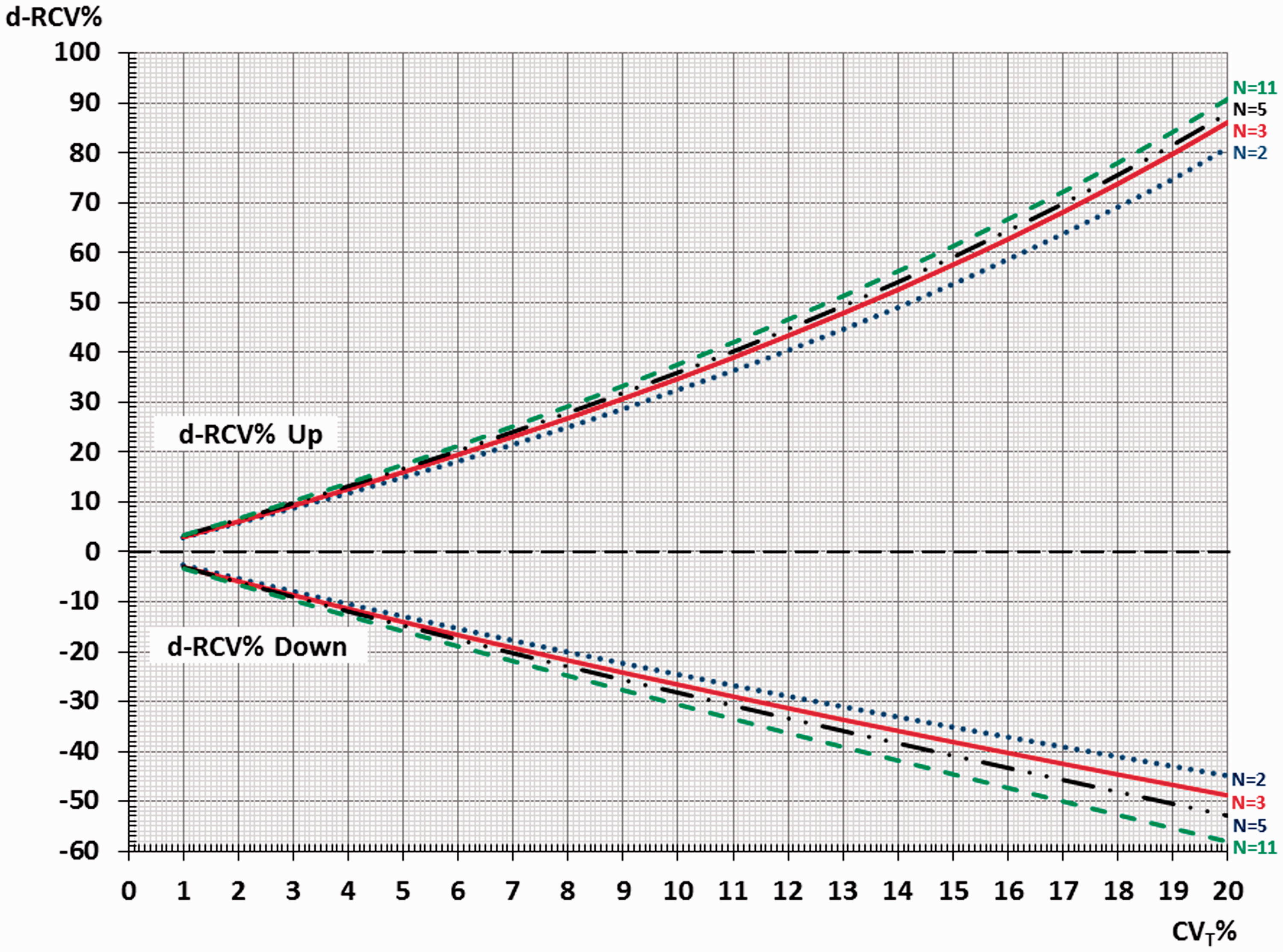
The dynamic RCV (d-RCV) values (based on RCF-factors in Table 1) are shown for both percentages of increase in results (d-RCV% Up) and percentages of decrease in results (d-RCV% Down). The graphs show the d-RCV values for the number of serial results (N = 2, 3, 5, 11) as a function of CV_T% (from 1% to 20%). N = 2 is blue (····), N = 3 is red (−−−), N = 5 is black (· · −− · ·), N = 11 is green (− − −).

N = 2

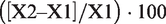
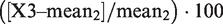
In the simulations and conversion calculations, the percentages difference between two results, X1 and X2, is calculated as

$$\left(\left[\text{X2}–\text{X1}\right]/\text{X1}\right)\cdot \text{1}00$$

N = 3

In the simulations for three results, X1, X2 and X3, the percentage difference is

$$\left(\left[\text{X3}–{\text{mean}}_2\right]/{\text{mean}}_2\right)\cdot \text{1}00$$

where mean₂ is the mean of X1 and X2.

N = 4 and N5–N11

For N = 4, the percentage difference is calculated in an analogous manner and for N = 5 to N = 11, mean₄ is maintained as a constant.

RCV calculations according to the proposal of Jones and Chung ⁶

This RCV concept uses n₁ as number of results before a clinical event and n₂ as the number of results after the event. In the RCV simulations, only the new result (n₂ = 1) is chosen and compared with the mean of the previous results (when n₁ is increasing from 1 to 10). ⁶ RCV formulae for RCV% Up and RCV% Down developed by Lund et al., ⁷ based on the model of Jones and Chung, ⁶ were used to generate the purple graphs in Figure 3 denoted ‘Jones and Chung ⁶ ’.

Figure 3.

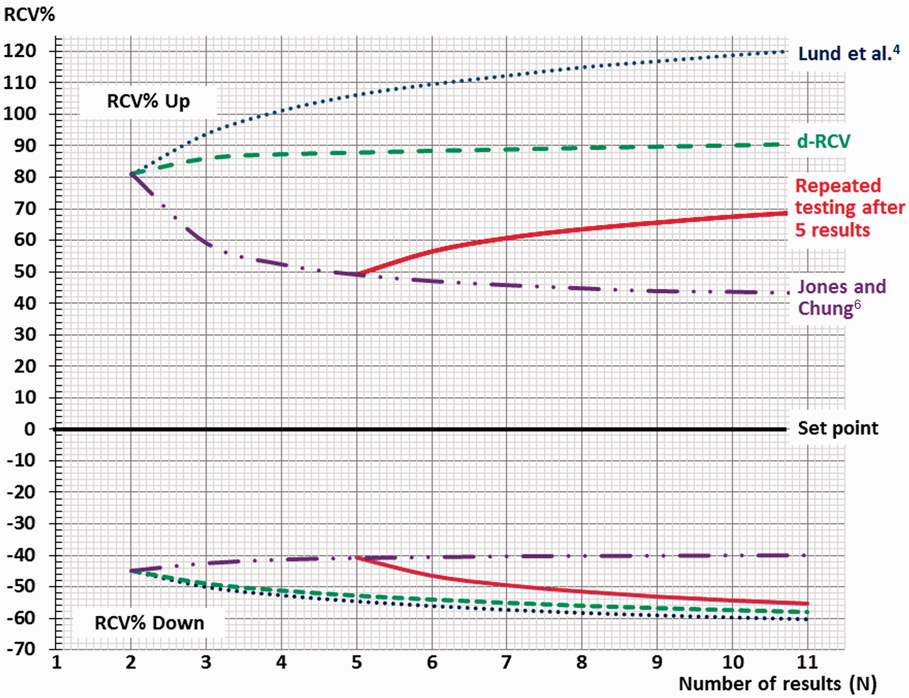
The RCV% Up and RCV% Down limits for significant differences as a function of number of results are presented as graphs from three serial RCV concepts, when CV_T = 20%. The green graphs (− − −) illustrate the dynamic RCV model (d-RCV), where the mean of the first results up to four results is an estimate of set-point following repeated testing. The blue graphs (····) represent the serial RCV concept of Lund et al., ⁴ where the first result is used as an estimate of a set-point and all subsequent results examined using repeated testing. The purple graphs (−− · · −−) represent the RCV concept of Jones and Chung, ⁶ where the mean of previous results is assumed as an estimate of set-point without ongoing assessment. The red graphs (−−−) combine the RCV concept of Jones and Chung ⁶ until four results are obtained and, as an example, use of the d-RCV concept with repeated testing from 5 to 11 serial results.

RCV calculations according to ‘Repeated testing after five results’ in Figure 3

With up to five serial results, the RCV concept is identical with the ‘Jones and Chung ⁶ ’ concept in Figure 3. From six serial results, the RCV concept is identical with d-RCV (i.e. all further results are compared with mean₄ in the calculations) and this is illustrated as the red graphs in Figure 3.

RCV calculations according to ‘Lund et al. ⁴ ’ in Figure 3

This RCV concept uses the first result as an estimate of the set-point. In the simulations, all further results were only compared with this fixed initial result when RCV calculations were made. Based on this model, the blue graphs in Figure 3 were generated.

RCV calculations according to ‘d-RCV’ in Figure 3

The green graphs in Figure 3 were generated using conversion from d-RCF to d-RCV%.

Results

In Table 1, the simulation results from the d-RCF_up2 factors for two serial results (N = 2), d-RCF_up3 for three serial results (N = 3) and on the remainder of the series up to d-RCF_up11 (N = 11) are provided as a function of CV_T%. Similarly, d-RCF_down factors for two, and up to 11 results, are also provided in the table.

Based on the same simulation results, Figure 2 is generated after transformation of the d-RCF values to d-RCV% for both percentages of increase in results (d-RCV% Up) and percentages of decrease in results (d-RCV% Down). The graphs show the d-RCV% values for number of serial results (N = 2, 3, 5, 11) as a function of CV_T% (from 1% to 20%). The similar RCV% Up and RCV% Down results are visualized as green graphs in Figure 3 as a function of the number of available serial results (from N = 2 to N = 11) for CV_T = 20%.

Discussion

RCV for two consecutive results

Recently, three groups of authors have reviewed the ‘common’ calculation of RCV and have obtained a consensus that it is incorrect to use CV.^2,9,10 In the theoretical ‘common’ (incorrect) RCV calculations, the limits for a significant increase and decrease are identical (symmetrical). But use of this ‘common’ RCV will generate more false-positive results than that expected in theory for increased concentrations over time and, as expected, will generate too few false-positive results when decreases occur, due to the skew (logarithmic) measured difference (X2–X1)/X1. Consequently, the correct RCV limits for CV must be higher for increased results and lower for decreased results compared with the ‘common’ symmetrical limits. This asymmetrical phenomenon of correct RCV limits is illustrated in Figure 2 (for N = 2, 3, 5 and 11) and in Figure 3 (with CV_T = 20% and N = 2, the RCV% Up = 81.1% and RCV% Down = −44.8%). A further consequence of the use of the correct asymmetrical limits is that it is more difficult to reveal an upward difference whereas downward differences are more easily detected. However, when small CV_T exist (less than 5%), the d-RCV% Up and d-RCV% Down are nearly symmetrical and become more asymmetrical as CV_T increases (Figure 2).

Problems in RCV calculations using more than two serial results (time series analysis)

As an example, Fraser ¹¹ has described a case of changes in liver function tests in a 63-year-old man who was prescribed a statin to lower his less-than-ideal serum cholesterol concentration. The serum aspartate aminotransferase (AST) activity rose with time (16, 18, 24, 40, 54, 69 U/L) over eight months. RCV calculation between successive pairs of serial results showed that two of the increases were not significant (and three of the increases were significant) at 95% probability, although the AST activity results rose from a ‘baseline’ of 16 U/L to 69 U/L after eight months. The RCV problem, with inconsistent interpretation of the significance of the differences seen, was obvious when the pattern of serial results was made of small differences in one direction and ended up far from ‘baseline’, then the RCV calculations did not flag any significance differences. This also illustrates the problem when serial results of a biomarker may have been generated too frequently in an individual. But, this RCV problem is solved by applying the d-RCV model which uses mean of the first four results, without significant changes, as a fixed set-point, and compares all the following results with this set-point. In this way, the significance limits are practically constant and even small persistent rises (or falls) will be flagged as significant changes over time.

Repeated testing applied to d-RCV

The d-RCV calculations are based on CV_T simulations. Therefore, the d-RCV limits (d-RCV% Up and d-RCV% Down in Figure 2) are asymmetrical due to skew measured (%) difference which arises using CV_T. In addition, repetitive testing is used in the d-RCV model, i.e. every time a new result is obtained, it is compared with previous results. In fact, the calculation determines whether this new result is significantly different from previous results. The use of repeated testing implies that the number of false-positive results increases. In the d-RCV model, repeated testing is compensated for by making the limits for a significant difference wider when more results are included, maintaining the false-positive rate at 2.5% in each direction, as also illustrated in Figure 3.

Interpretation of changes in serial results using d-RCV

If the first four results are within the limits calculated for detection of differences, a steady state with a homeostatic set-point as the mean₄ of four results is verified with a probability of 95%. Further results (N = 5, 6,…) within the limits given in Table 1 confirm the set-point. Although the determination of set-point is confirmed, additional results (N = 5, 6, …) increase the number of false-positive results and, to maintain 5% false-positive results, the limits must be wider (Table 1). If a new result is outside the limits, the steady state situation has ended and this biomarker result could then be the first result in estimation of a new homeostatic set-point. To determine a possible new set-point, four additional results are then needed. In assessment of new biomarker results compared with former results, the d-RCV model is designed to be user-friendly. No calculations of d-RCF or d-RCV% are needed. Given the number of results (N) and CV_T%, the actual d-RCF is listed in Table 1 or the corresponding d-RCV% is interpolated from the graph shown in Figure 2. Then, the limits for significant differences (up or down) can (simply) be calculated by multiplying the actual d-RCF factor with the mean of the previous results (mean₄). Similarly, percentages (using d-RCV%) to calculate the limits for significant differences (up or down) are compared with the mean of the previous results (up to mean₄ for four results and with mean₄ for additional results) as interpolated from Figure 2. The advantage of using d-RCV is that when (minor) increases or decreases of a biomarker are difficult to assess, then the d-RCV calculations will objectively determine whether the differences in serial results are significant or insignificant.

Examples in testing for steady state using d-RCV

Two constructed examples of the application of the d-RCV model on seven and eight results for HbA1c concentration from two diabetic patients over two years are illustrated in Figure 4(a) and (b). CV_T is assumed to be 8%. In Figure 4(a), it should be noted that the limits for significant differences are increased from 60 mmol/mol up to the fifth result and then the limits approach horizontal straight lines for the sixth and seventh result. According to the d-RCV model, the variation in results from this patient is interpreted as having a homeostatic set-point (=mean₄) and is considered to be in steady state over the monitoring period with a probability of 95%. In Figure 4(b), the patient had a significant increase in HbA1c from the first (60 mmol/mol) to the second result (85 mmol/mol). Therefore, the patient was not in steady state during this time. In contrast, throughout the period from the second (85 mmol/mol) to the last result (73 mmol/mol), this patient was in steady state for HbA1c and had a set-point (77.5 mmol/mol). The associated d-RCV calculations are provided in Table 2.

Figure 4.

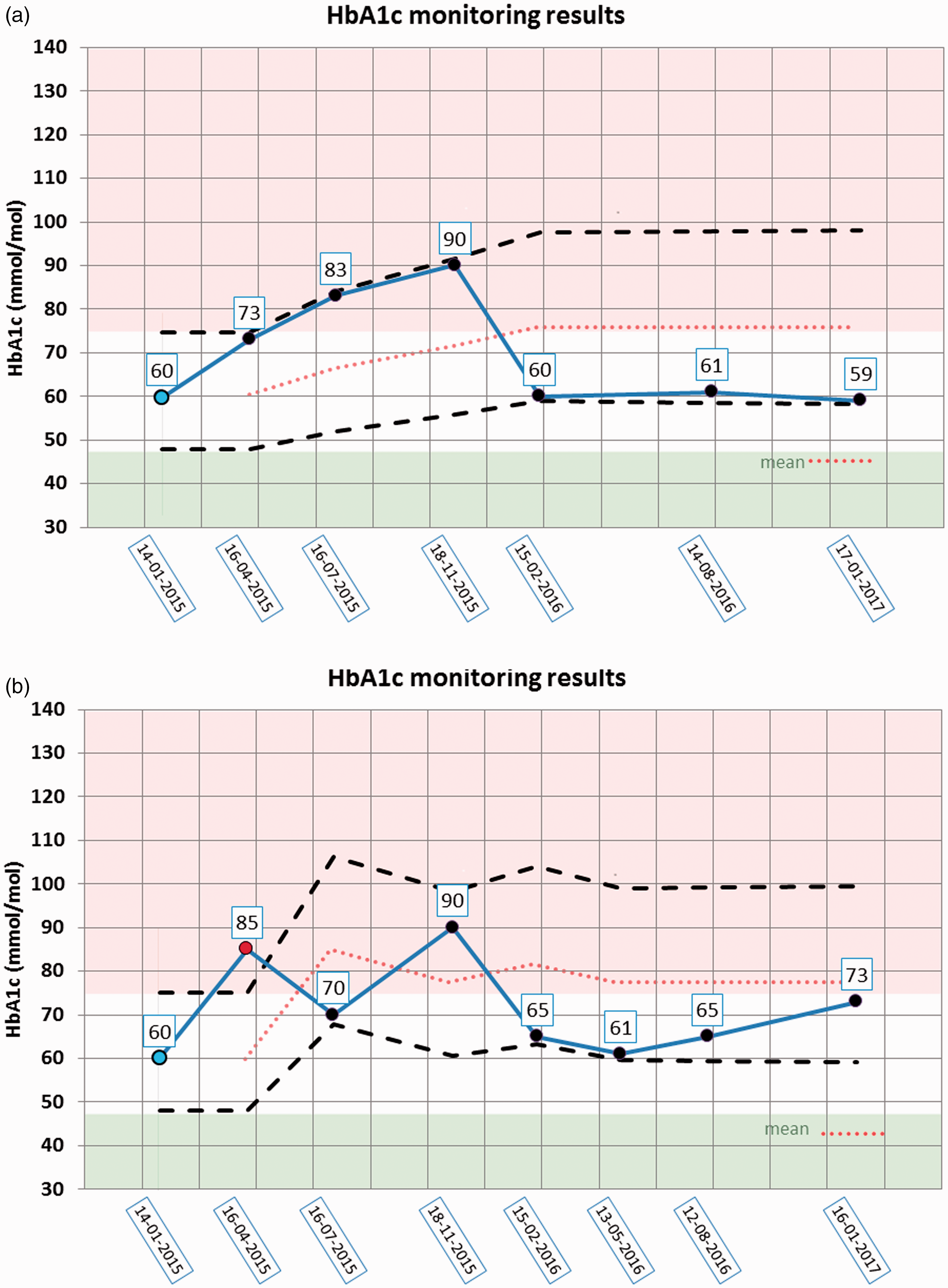
(a and b) Examination for steady state of HbA1c using the d-RCV model. Two patients have had seven and eight samples for examination of HbA1c (mmol/mol) over two years for monitoring of diabetes. The dotted lines show the upper and downward limits for remaining in steady state and are calculated in Table 2. Upper on the circles show the actual results of HbA1c. Start point (blue bullet), point outside steady state and used for new start (red bullet), points within steady state (black bullets). Green area (HbA1c< 48 mmol/mol) are normal values, white area (48<HbA1c < 75 mmol/mol) are therapeutic appropriate values for stable diabetes patients and red area (75<HbA1c mmol/mol) are too high values and which should be avoided.

Table 2.

Two constructed examples of calculated d-RCV upper and downward limits for assessment of homeostatic set-point and steady state in HbA1c (mmol/mol) results from two diabetic patients (also illustrated in Figure 4(a) and (b)).

HbA1c (mmol/mol):	Results	Mean	Upper limit (d-RCFup · mean)	Downward limit (d-RCFdown · mean)
Figure 4(a)	X1 = 60
	X2 = 73	60.00	1.250 · 60.00 = 75.0	0.7990 · 60.00 = 47.9
	X3 = 83	66.50	1.268 · 66.50 = 84.3	0.7828 · 66.50 = 52.1
	X4 = 90	72.00	1.274 · 72.00 = 91.7	0.7755 · 72.00 = 55.8
	X5 = 60	76.50	1.278 · 76.50 = 97.8	0.7703 · 76.50 = 58.9
	X6 = 61	76.50	1.281 · 76.50 = 98.0	0.7660 · 76.50 = 58.6
	X7 = 59	76.50	1.284 · 76.50 = 98.2	0.7625 · 76.50 = 58.3
Figure 4(b)	X1 = 60
	X2 = 85 a	60.00	1.250 · 60.00 = 75.0	0.7990 · 60.00 = 47.9
	X3 = 70	85.00 a	1.250 · 85.00 = 106.3	0.7990 · 85.00 = 67.9
	X4 = 90	77.50	1.268 · 77.50 = 98.3	0.7828 · 77.50 = 60.4
	X5 = 65	81.67	1.274 · 81.67 = 104.1	0.7755 · 81.67 = 63.3
	X6 = 61	77.50	1.278 · 77.50 = 99.1	0.7703 · 77.50 = 59.7
	X7 = 65	77.50	1.281 · 77.50 = 99.3	0.7660 · 77.50 = 59.4
	X8 = 73	77.50	1.284 · 77.50 = 99.5	0.7625 · 77.50 = 59.1

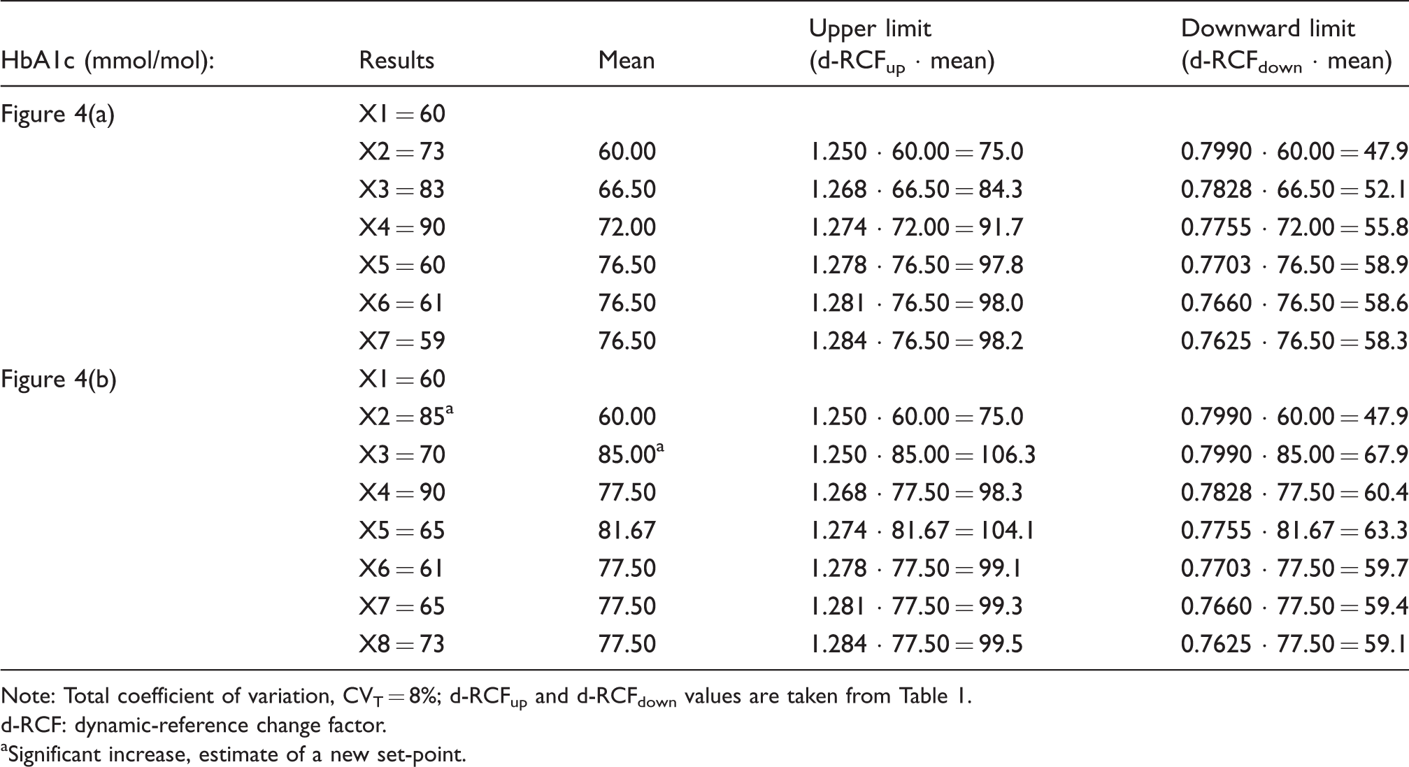
Note: Total coefficient of variation, CV_T = 8%; d-RCF_up and d-RCF_down values are taken from Table 1.

d-RCF: dynamic-reference change factor.

^aSignificant increase, estimate of a new set-point.

d-RCV vs the Lund et al. ⁴ RCV concept

In Figure 3, d-RCV is shown as the green graphs. In Figure 3, the blue graphs for RCV% Up and RCV% Down from the concept of Lund et al. ⁴ using (only) the initial concentration with subsequent testing are also shown. For RCV% Up for more than two results, the (blue) curve is considerably higher than the similar curve from d-RCV (green) because the serial blue results are compared with an uncertain initial result as an estimate of the set-point, whereas the d-RCV curve (green) is based on a more accurate dynamic estimation of set-point based on the first four results. A consequence of these differences is that the percentages of increased results between the green and blue curves are considered as significant using d-RCV and not significant using the concept of Lund et al. ⁴ Conversely, for decreases in results (RCV% Down), the model of Lund et al. ⁴ (blue curve) and d-RCV (green curve) performs similarly (Figure 3).

d-RCV vs the Jones and Chung ⁶ RCV concept

The purple graphs in Figure 3 represent the RCV calculated from the concept of Jones and Chung. ⁶ In this version of their RCV concept, steady state is assumed of, e.g. up to 10 serial results before a clinical event and only one result after an event. In other words, after a clinical event, the purple graphs in Figure 3 illustrate the limits for one new result to be assessed as a significant difference as compared with estimation of the set-point based on serial results before the event. In comparison with the green d-RCV model, the RCV model of Jones and Chung ⁶ assumes steady state (an assumption – which is not examined) and, therefore, has narrower limits for significant differences with additional number of serial results (purple graphs vs. green graphs in Figure 3). However, we believe that clinicians usually assess new biomarker results in an individual and compare them with previous results, continuously. It should be emphasized that the previous results must not be compared with new results (as repeated testing) when applying the RCV concept of Jones and Chung ⁶ because, then, the number of false-positive results obtained will considerably change the limits for significant differences. This phenomenon is illustrated in Figure 3 with the purple graph and can be regarded as a combination of the concept of Jones and Chung ⁶ for the first results and repeated testing after five results as assessed using the d-RCV concept (i.e. the mean of first four results is used as a constant set-point [mean₄] and further results are compared with this set-point in the calculations). As a consequence of this repeated testing, the red graphs immediately differ from the purple graphs after five results (Figure 3). In this way, the presented d-RCV model using repeated testing is more comparable to clinical practice.

Repeated testing always increases the number of false-positive results

When a test is going to be applied the number of false-positive results that is considered acceptable requires careful considerations. Usually, 5% false-positive results are accepted. If a test is repeated, an increased number of false-positive results is obtained. And, if the new test is independent from the first, the per cent of false-positive results can be calculated using the following formula: FP% = 100–100(1–p)^m, where FP% is the number false-positive results in percentage terms, p is the number of false-positive results from one test and m is number of independent repeated tests. ¹² So, if we repeat a test with 5% false-positive results (P = 0.05), 10% false-positive results are obtained, minus in the few cases in which both tests are positive simultaneously, i.e. the cumulated number of false-positive results is 9.75% using the formula. If the test is repeated 14 times, then the number of cumulated false-positive results is 51.23% using the formula, i.e. the probability to obtain one false-positive result after 14 tests is 51.23%. Expressed in a thought-provoking manner, instead of performing 14 tests a coin could be simply tossed – and the probability would be similar (50%). Accordingly, if a test for which the results is negative is repeated often, the results will become (false) positive.

The formula for FP% can also be applied in RCV calculations. An example: the results are normally (Gaussianly) distributed using SD (in steady state situation) and only significant increases in concentrations (U/L) are calculated. Given are SD = 20 U/L, Z = 1.96, set-point = 100 U/L which gives RCV Up = 55.4 U/L. So, when two independent results (X1 and X2) are generated, a false-positive increase will occur if X2–X1 > 55.4 U/L. When two new independent results (X3 and X4) are available, a new independent RCV test can be performed and using the formula; FP = 4.94%. Similar calculations of FP% for independent results have been produced using simulations and the same results were obtained as found using the formula (data not shown). If the corresponding FP% for four results are calculated and d-RCV concept is applied with constant upper limit for increases (RCV = 55.4 U/L), the FP% is lesser than for independent results. The explanation is that d-RCV applies repeated RCV testing, but the results are not independent, because new results are compared with previous results. If similar FP% calculations are performed using Jones and Chung ⁶ RCV concept, small FP% will be obtained when using more results (Table 3). The explanation is that Jones and Chung ⁶ only use one RCV test when obtaining more results (Table 3). An example: when four results are obtained (X1, X2, X3 and X4), Jones and Chung ⁶ only record significant increases if X4–1/3(X3 + X2 + X1) > 55.4 U/L. This implies that X2 must not be compared with X1 and X3 must not be compared with either X2 or X1. In consequence, for four results, FP = 0.82% using one RCV test from Jones and Chung ⁶ and FP = 4.46% using d-RCV (with three repeated RCV tests, Table 3). However, which concept should be used in clinical practice?

Table 3.

False-positive results in per cent (FP%) calculated with use of d-RCV and the Jones and Chung ⁶ RCV concept (the last result is compared with mean of previous results).

N	2	4	6	8	10
FP% d-RCV	2.51 (1)	4.46 (3)	5.70 (5)	6.85 (7)	8.00 (9)
FP% Jones and Chung 6	2.51 (1)	0.82 (1)	0.56 (1)	0.47 (1)	0.45 (1)

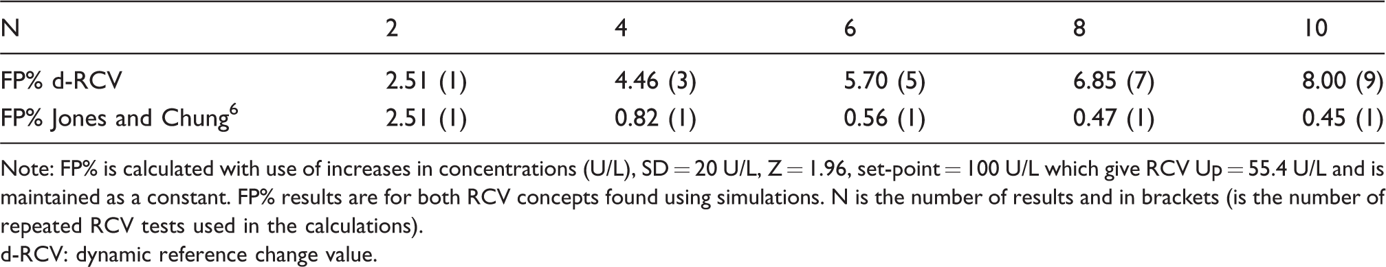
Note: FP% is calculated with use of increases in concentrations (U/L), SD = 20 U/L, Z = 1.96, set-point = 100 U/L which give RCV Up = 55.4 U/L and is maintained as a constant. FP% results are for both RCV concepts found using simulations. N is the number of results and in brackets (is the number of repeated RCV tests used in the calculations).

d-RCV: dynamic reference change value.

In the following example, the way in which a clinician interprets results of a biomarker is considered. In this example, the clinician only is interested in possible increasing results. When the clinician obtains a new result (X2), the clinician might well compare the result with a previous result (X1). If X2–X1 < an upper intuitive (‘RCV’) limit, then the X1 and X2 are similar (first ‘RCV’ test). The clinician has established this ‘RCV’ limit based on many years of clinical experience. Later, the clinician will obtain a third result (X3) and compare it with the previous results (X2 and X1). If X3 is unexpectedly significant higher than X1 and X2 (second ‘RCV’ test), a further investigation may well be requested (X4). If X4 is similar with X1 and X2 (third ‘RCV’ test), X3 might be considered as a laboratory error. Nevertheless, X3 could well be a false-positive result. In this case, the clinician undertook (probably without knowing) repeated ‘RCV’ testing three times and ought to have considered that the probability of obtaining false-positive results during this process had risen considerably.

The initial intuitive impression could be that further results and RCV tests make the measurements uncertain due to the increased number of false-positive results. But, the design of d-RCV takes care of this increase. Therefore, the second more reflective impression could be that more results make the data interpretations more certain using d-RCV. In other words, further results on a biomarker, which are within the limits given from d-RCV, confirm that the patient is indeed in steady state.

RCV calculations based on SD and changes in differences vs. RCV calculations based on CV and changes in percentage terms

In the example mentioned previously, SD = 20 U/L and increase in concentrations (U/L) for the RCV calculation were used. When the set-point =100 U/L and RCV = 55.4 U/L, then the RCV Up = 55.4%. In Figure 3 and in Table 1, it is shown that the corresponding RCV Up = 81.1% using CV_T = 20%. Obviously, there is a marked increase in RCV% Up using CV_T and this phenomenon is caused by general problems with per cent calculations. A simple example illustrates the problem: a rise from 10 to 50 U/L (40 U/L) is an increase of 400%, whereas an apparently larger rise from 100 to 150 U/L (50 U/L) is only an increase of 50%. These results in percentage terms demonstrate the problem with low values in percentage term calculations, i.e. when low values near zero are included in the denominator. The similar problem is clear, when RCV is calculated with low initial concentration using CV_T% and causes the asymmetrical limits for RCV% Up and RCV% Down (Figure 3, Table 1). This asymmetrical problem is not seen using SD and differences in concentrations when RCV is calculated. On the other hand, (nearly) all biological variations data are given as CV% and, therefore, the d-RCV may be used.

Other factors affecting the RCV calculations

With the use of CV for biological variation, some biomarkers fail to meet the assumption of homogeneity of variance, i.e. the biological variation data applied could be more individual. The clinician ought also to note that some biomarker results could be analysed on different equipment and the analytical variation could be different. Furthermore, the assumption for RCV calculations is that the results are normally (Gaussianly) distributed but many biomarkers follow a logarithmic normal (log Gaussian) distribution.

Thus, many assumptions should be fulfilled before using RCV (and d-RCV). Nevertheless, with use of d-RCV, the clinician has an objective tool to measure when results of a biomarker show that a patient is in steady state or otherwise.

Conclusions

Use of the ‘common’ RCV based on two consecutive results is incorrect when CV_T are used.

This ‘common’ RCV is inconsistent in interpretations when applied to more than two serial results in an individual.

The developed dynamic model (d-RCV) for more than two serial results, based on CV_T simulations, gives clear and correct answers to the interpretation of differences in serial results.

In the d-RCV model, every new result is tested for steady state and the mean of previous results are used as an estimate of the homeostatic set-point.

When the first four results are in steady state, the mean is used as the set-point for assessment of further results.

The d-RCV model compensates for the increasing number of false-positive results which occur due to the repeated testing for steady state.

If a difference is significant, then the steady state has ended and the new result could be an estimate of a new set-point and the analysis of possible differences begun again.

The d-RCV model is convenient for ongoing testing for steady state of a biomarker in the monitoring of an individual.