
Abstract
Background
Reference change values provide objective tools to assess the significance of a change in two consecutive results for a biomarker from an individual. The reference change value calculation is based on the assumption that within-subject biological variation has random fluctuation around a homeostatic set point that follows a normal (Gaussian) distribution. This set point (or baseline in steady-state) should be estimated from a set of previous samples, but, in practice, decisions based on reference change value are often based on only two consecutive results. The original reference change value was based on standard deviations according to the assumption of normality, but was soon changed to coefficients of variation (CV) in the formula (reference change value = ± Z ċ 2½ ċ CV). Z is being dependent on the desired probability of significance, which also defines the percentages of false-positive results. The aim of this study was to investigate false-positive results using five different published methods for calculation of reference change value.
Methods
The five reference change value methods were examined using normally and ln-normally distributed simulated data.
Results
One method performed best in approaching the theoretical false-positive percentages on normally distributed data and another method performed best on ln-normally distributed data. The commonly used reference change value method based on two results (without use of estimated set point) performed worst both on normally distributed and ln-normally distributed data.
Conclusions
The optimal choice of method to calculate reference change value limits requires knowledge of the distribution of data (normal or ln-normal) and, if possible, knowledge of the homeostatic set point.
Keywords
Introduction
Reference change values (RCVs), also known as critical differences, are tools to assist with objective analysis of differences in the results of two consecutive measurements of a biomarker in an individual. The basis for this aid to interpretation is that, for a difference in serial results to be significant, this must be greater than the inherent variation. The most commonly cited and applied formula for calculating RCV limits is RCV = ± [Z ċ 2½ ċ (CVA2 + CVI2)½], where CVA is the analytical coefficient of variation (CV) and CVI is the within-subject biological variation. Often, the formula is given as RCV = ± [Z ċ 2½ ċ CVT], where CVT is the total CV, CVT = (CVA2 + CVI2)½. Z is the number of standard deviations appropriate to the probability desired for detecting differences. Usually, 95% probability (P < 0.05 when 5.0% are false-positives) is regarded as significant, and 99% probability (P < 0.01 when 1.0% are false-positives) is highly significant. Thus, in general, 1.65 and 2.33 are the appropriate Z-scores to use for a unidirectional change, i.e. when increases or decreases in concentration are being considered (one-tailed). However, before applying the RCV calculation for interpretation of the difference in two results, the assumptions inherent in the calculation of RCV should be considered. The RCV calculation is based on the assumption that CVI represents random fluctuation around a homeostatic set point and follows a normal (Gaussian) distribution. This set point (or baseline in steady-state) ideally should be estimated from more than one sample, but in practice, RCV calculations often are based on only two consecutive results. In consequence, the percentage of false-positive results will differ from the theoretical. This fact was observed in 2015, when we studied methods to calculated limits for significant uni- and bidirectional differences in two or more serial results of a biomarker based on a computer simulation model.1,2 During this work, we observed that the percentages of false-positive results from simulated data-sets were greater than those calculated theoretically for an increase in concentration and less for a decrease in concentration.
Harris and Yasaka, 3 described the first application of RCV where for two consecutive results, X1 and X2, the significant limits for a change in concentration are: X2 − X1 = ± Z ċ 2½ ċ SDT, where SDT is the total standard deviation (SD) of analytical (SDA) plus within-subject biological variation (SDI), [SDT = (SDA2 + SDI2)½]. Shortly after, Costongs et al. 4 expanded the concept to alternate between SD and CV in calculation of RCV. In making this change, an important factor has turned out to be the value used to change the difference in results (in the assay units) into a per cent difference, as differences in the choice of this value give different percentage changes for the same difference in assay units. Fraser and Harris 5 redefined RCV through using CV instead of SD as: RCV = ± [Z ċ 2½ ċ (CVA2 + CVI2)½] and included a table and a formula where the number of specimens required to assess the homeostatic set point at different levels of analytical imprecision were specified. This approach uses the set point (mean of baseline results) to convert the difference in results to a percentage change. However, the common use of RCV is based on only two results and comparison of the difference to the first result (i.e. the first result is an estimate of the set point, albeit rather uncertain). In this process, one important assumption for RCV is altered in that CV is considered to be the constant rather than SD and, in consequence, the original RCV calculation method 3 should be modified. Jones 6 pointed out the problem with the assumption of constant SD and revised the RCV calculations with the assumption of constant CV. Consequently, Jones postulated new RCV limits based on a formula detailed without rigorous mathematical explanation. We recently discovered, using the same assumptions, that our calculated limits for significant changes in two results based on a computer simulation model were in perfect agreement with the mathematically calculated RCV limits from Jones.1,2 Thus, it seemed that the assumptions applied (e.g. constant CV or constant SD) for calculation and application of the different RCV methods are very important.
The RCV calculations also assume that CVI shows a normal (Gaussian) distribution. However, it has become more and more apparent that, for many measurands, within-subject variations are more appropriately described as ln-normal distributions. A data-set is ln-normally distributed if the natural logarithms of that data-set are normally distributed. For example, Fokkema et al. 7 found that the CVI distribution of brain natriuretic peptides showed a right-skewed distribution and developed an RCV calculation method by addressing the skewness of the distribution. Therefore, Fokkema et al. 7 stated more correct formulae for RCV calculations when a data-set is ln-normally distributed.
The aim of this study was to investigate the performance of five published calculation methods for RCV applied to normally and ln-normally distributed simulated data appropriate to apparently healthy individuals. The performance of the RCV methods was assessed by simulations and the percentages of false-positive results for each method calculated and then compared to the theoretical percentages. The RCV performance was investigated by varying both CVT and percentages of theoretical results (i.e. use of different Z-scores). Based on the simulation results, an optimal choice of RCV method is possible, depending on whether the distributions of the data are normal or ln-normal or unknown and whether the homeostatic set point is known or unknown.
Materials and methods
All data for the simulations were generated using Microsoft Excel version 2010.
RCV calculation methods
For two consecutive results, X1 and X2, five methods for calculating RCV were studied. Four methods use the formula [(X2 − X1)/Y] = RCV for a change in concentration, where the value of Y is dependent on the method.
RCV method ‘Common’ 8
([X2 − X1]/Y) = ([X2 − X1]/X1) = RCV = ± Z ċ 2½ ċ CVT are the limits for a difference in concentration. In this method, Y = X1 and is the first result and the only estimate of the mean of the individual’s homeostatic set point.
RCV method ‘Sölétormos’ 9
([X2 − X1]/Y) = (X2 − X1)/(0.5 ċ [X1 + X2]) = RCV = ± Z ċ 2½ ċ CVT are the limits for a difference in concentration. In this method, Y = 0.5 ċ (X1 + X2), and the mean is an estimate of the individual’s homeostatic set point.
RCV method ‘Fraser’ 5
([X2 − X1]/Y) = RCV = ± Z ċ 2½ ċ CVT are the limits for a difference in concentration. Y is the individual’s homeostatic set point and is estimated as a mean of further serial results. The number of specimens required for a confident estimate of the homeostatic set point is n = (Z ċ CVT/D) 2 , where n is the number of specimens required and D is the desired percentage closeness to the homeostatic set point.
RCV method ‘Jones’ 6
[(X2 − X1)/Y] = [(X2 − X1)/X1] = RCV = {#x02212; (CVT)2 ± [(CVT)4 – 2 ċ (CVT)2 ċ ((CVT)2 – 1/Z2)]½}/((CVT)2–1/Z2) are the limits for a difference in concentration. Y = X1 is the first result and is the only estimate of the mean of the individual’s homeostatic set point.
RCV method ‘Fokkema’ 7
X2/X1 = exp(±Z ċ 2½ ċ σ) are the limits for a difference in concentration where σ = [ln((CVT)2 + 1)]½. X1 is the first result and is the only estimate of the mean of the individual’s homeostatic set point.
These five described RCV calculations were used on normally and ln-normally distributed data generated from simulations. The RCV limits were calculated using Z = 1.65 and 2.33 corresponding to theoretical unidirectional percentage of false-positive results of 5.00% and 1.00%, respectively. The RCV were calculated for CVT = 5.0%, 10.0%, 15.0% and 20.0% (representative of most often encountered values in everyday practice calculations of RCV). It should be noted that CVT for ln- normally and CVT of the underlying normally distributed data are not the same. The CVT for ln-normal distributions is calculated using CVT = [exp(σ2) − 1]½, where σ2 is the variance of the underlying normal distribution. 7 A total of 10,000 simulated normally and ln-normally distributed results, as would be found in apparently healthy individuals, were generated for each CVT. The method to estimate percentages of false-positive results has been described in detail in a previous publication. 1
Results
Estimation of false-positive results when unidirectional RCV a were calculated using five different methods on simulated concentration data as from apparently healthy individuals with varying coefficients of variation and theoretical false-positive results.
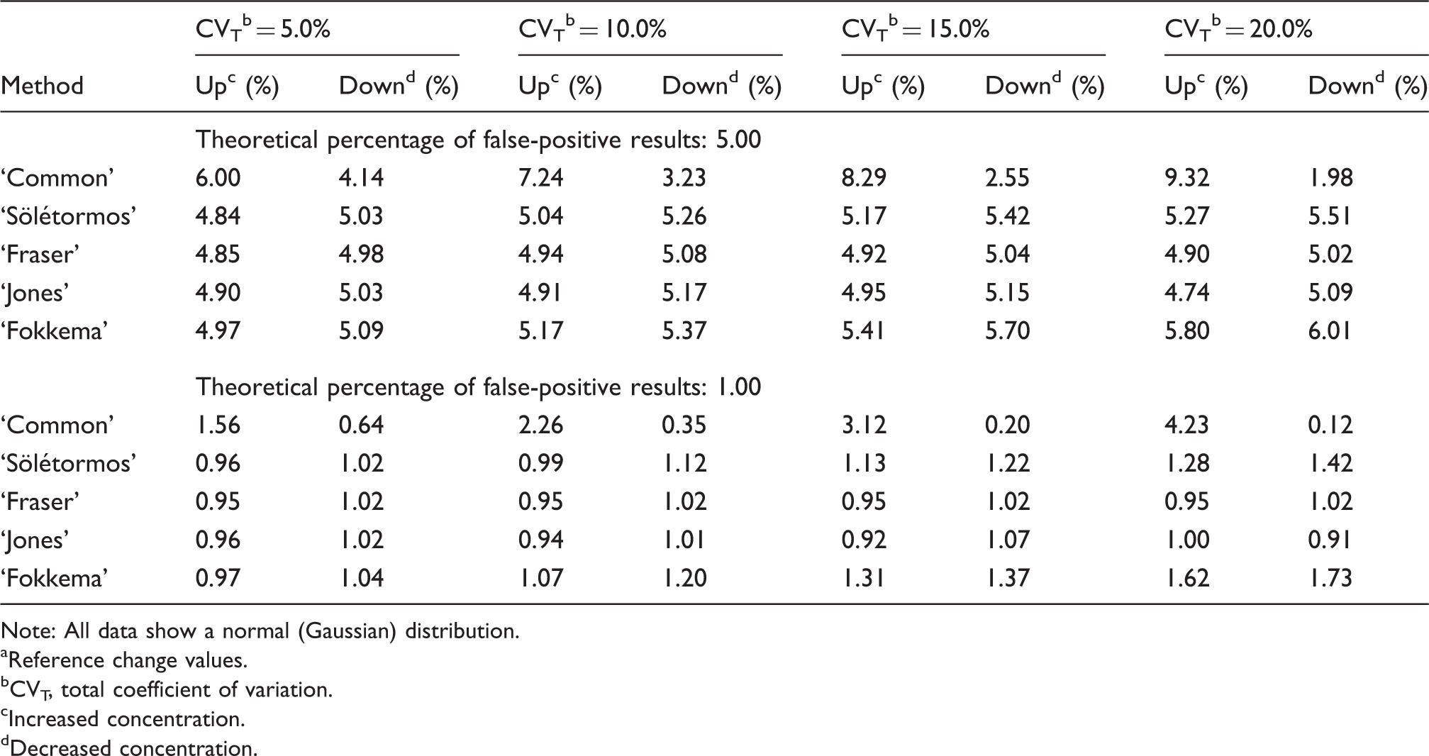
Note: All data show a normal (Gaussian) distribution.
Reference change values.
CVT, total coefficient of variation.
Increased concentration.
Decreased concentration.
Estimation of false-positive results when unidirectional RCV a were calculated using five different methods on ln-normally distributed simulated concentration data as from apparently healthy individuals with varying coefficients of variation and theoretical false-positive results.
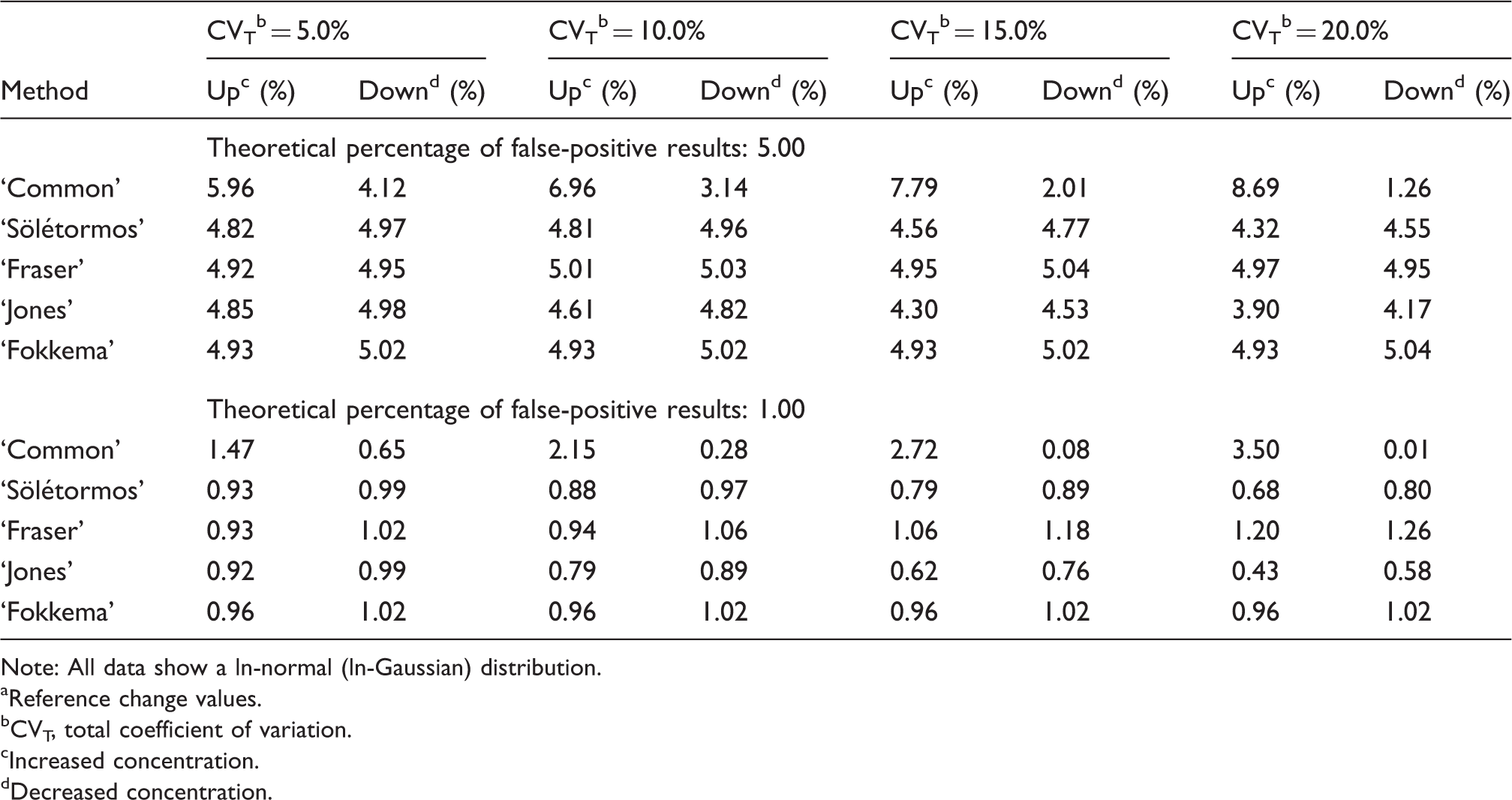
Note: All data show a ln-normal (ln-Gaussian) distribution.
Reference change values.
CVT, total coefficient of variation.
Increased concentration.
Decreased concentration.
Discussion
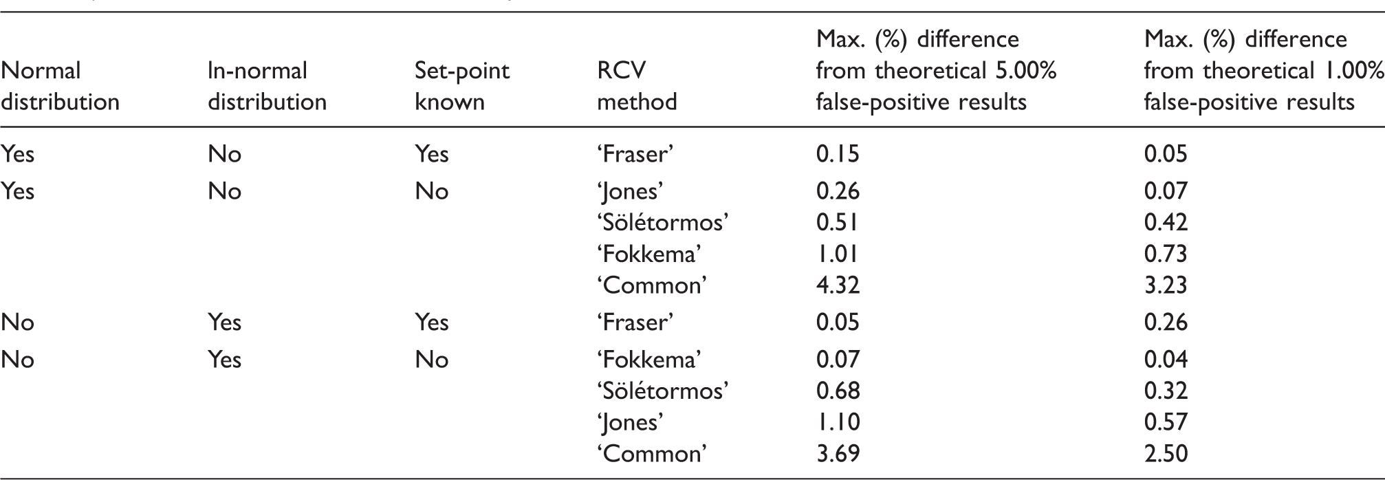
Estimated maximal difference from the expected theoretical percentages of false-positive results (5.00 and 1.00) using five reference change value (RCV) calculation methods (unidirectional), when the data display a normal (Gaussian) or ln-normal (ln-Gaussian) distribution, and the homeostatic set-point is known or unknown, and, the total coefficient of variation, CVT ≤ 20%.
Normal (Gaussian) distribution, Table 1
RCV method ‘Common’
The percentage of false-positive results was always greater than theoretical for increased concentration: i.e. using this RCV ‘Common’ method will always generate more false-positive results than expected. For example, the percentages of false-positive results were increased from 6.00 to 9.32% for an expected theoretical false-positive result of 5.00%, when CVT was increased from 5.00 to 20.00%. In contrast, the ‘Common’ method generated fewer false-positive results than theoretical when the concentration decreased. For example, the percentages of false-positive results were decreased from 4.14 to 1.98% for an expected theoretical 5.00%, when CVT was increased from 5.00 to 20.00%, respectively. This distortion of false-positive results is a consequence of changing the calculation formula from constant SD to constant CV and using the first result as a rough estimate of the homeostatic set point. In other words, a difference of two results (X2 − X1) is transformed from a linear scale to a new scale when the difference is related to the first result (i.e. [X2 − X1]/X1 = X2/X1 − 1). For increased concentrations, this new scale (X2/X1 − 1) is greater than a linear scale (and is more like a logarithmic function because X2/X1 has a logarithmic scale). Consequently, for increased concentrations, the ‘Common’ RCV method produces, relatively, more false-positive results when CVT is increased, and less for decreased concentrations. In our comparison of the tested five RCV methods, the ‘Common’ method performed worst, and in consequence, is not optimal as a method to calculate significant limits for differences in concentration of a biomarker in serial results from an individual.
RCV method ‘Sölétormos’
Compared with ‘Common’, the ‘Sölétormos’ method had better performance (max differences: 0.51%, Table 3). The ‘Sölétormos’ RCV method uses the mean of two results and thereby compensates for extreme results and leads to a better estimate of the homeostatic set point.
RCV method ‘Fraser’
Of the five RCV methods ‘Fraser’ method performed best, i.e. the percentages of false-positive results were very close to the theoretical values (max differences: 0.15%, Table 3). On the other hand, this good performance is dependent on a reliable estimate of the homeostatic set point. Therefore, associated with the description of the RCV method, a formula was stated with the number of specimens required to ensure that the mean result is, e.g. ± 5.00% of the individual’s homeostatic set point. 5 The ‘Fraser’ method is based on the original RCV concept from Harris and Yasaka, 3 i.e. a calculation of a significant difference of two consecutive results (X1 and X2). When RCV is calculated using CVT instead of original SDT, this difference should be compared with the homeostatic set point (Y), i.e. RCV = (X2 − X1)/Y. In this process, the SDT value is still a constant, mathematically, and the good performance results of the simulations from ‘Fraser’ method (Table 3), thus indicate that the original RCV concept from Harris and Yasaka 3 was correct.
RCV method ‘Jones’
The ‘Jones’ RCV method performed nearly as well as the ‘Fraser’ method (max differences: 0.26%, Table 3). The strength of the ‘Jones’ method is that knowledge of homeostatic set point is not required. ‘Jones’ method applies the same procedure as the ‘Common’ method by using the first result (X1) as an estimate of the homeostatic set point, [(X2–X1/X1]), but compensate the distortion of false-positive results by extending the significant limits for an increase in concentration, and, lowering for a decrease in concentration (see section RCV method ‘Common’ above). Thus, the ‘Jones’ method has greater significant limits for increased concentrations compared with both ‘Common’ and ‘Fraser’ RCV methods. Consequently, the use of ‘Jones’ and ‘Fraser’ RCV method (both with comparable good performances, Table 3) on two serial results from an individual could lead to different interpretations. Therefore, if the homeostatic set point from an individual is available, it should be applied in the ‘Fraser’ RCV method, and if the set point is unknown the ‘Jones’ method is recommended. Jones
6
did not fully document the mathematical explanations and calculations for the RCV limits but these are now stated here. A mathematical formula for RCV can be generated by changing the original RCV calculation from constant SD to constant CV using the following: from X2 − X1 = Z ċ 2½ ċ SDT to (X2 − X1)/X1 = RCV = Z ċ ([SD1/X1]2 + [SD2/X1]2)½, where SD1 is the SD for the first result and SD2 is the SD for the second result. From this, equation can be derived X2 = (1 + RCV) ċ X1 and SD1/X1 = CVT and SD2 = CVT ċ X2 (CVT is considered as a constant) and these are substituted into the equation which is derived as: RCV = Z ċ ([CVT]2 + [1 + RCV]2 ċ [CVT]2)½. The latter equation can be considered as a quadratic with two solutions, one for an increase and one for a decrease in concentration. Jones realized the RCV calculation becomes ‘a little more complex’ and documented calculated RCV limits for limited CVT values in a Table. For practical use, we have created Figure 1 for further CVT values, where all the associated RCV limits can be read directly.
Illustration of bi-directional RCV limits for two consecutive measurements in accordance with ‘Jones’ for normal (Gaussian) distributions.
6
(a) is a larger version of a component of (b). RCV% up is the limit for a significant increase and RCV% down is the significant limit for a decrease in concentration as a function of CVT%. The RCV limits can be read for 90%, 95% or 99% probability.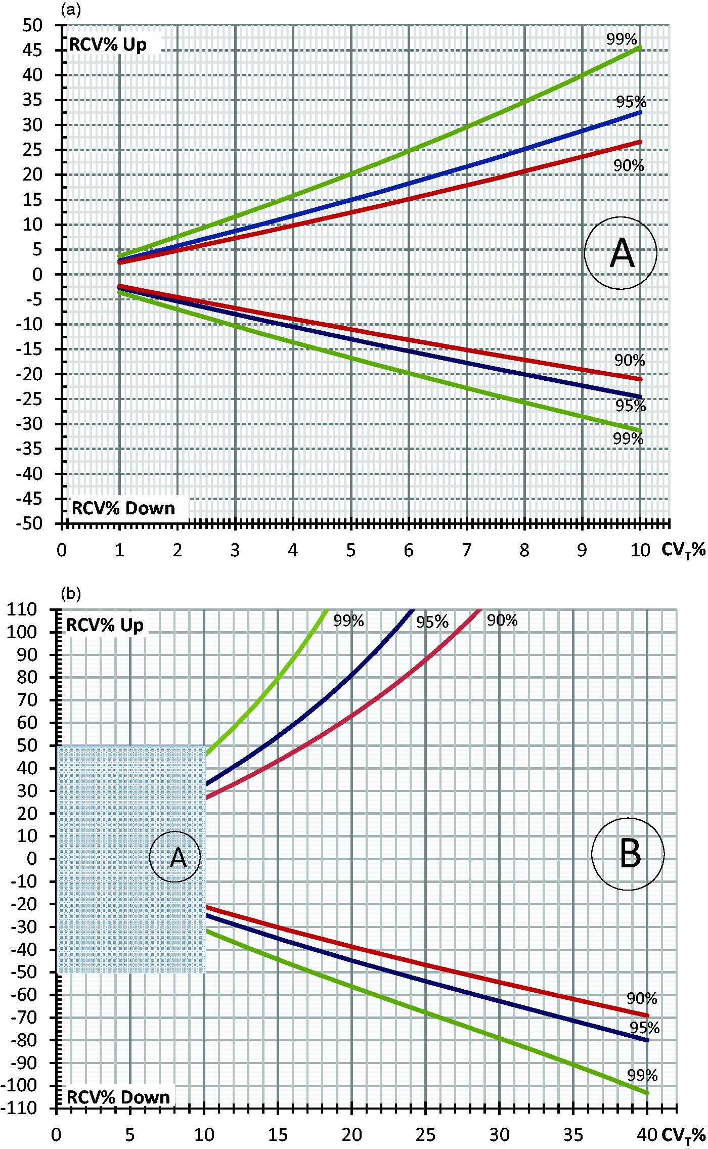
RCV method ‘Fokkema’
The ‘Fokkema’ RCV method is designed for ln-normal distributed data and produced more false-positive results than theoretical expected for both increased and decreased differences in concentration. Notably, the Fokkema method worked better with smaller CVT than with higher. This is expected as ln transformation of data sets with a narrow variation has less effect on the shape of the distribution.
ln-normal (ln-Gaussian) distribution, Table 2
RCV method ‘Common’
As with normally distributed data, the ‘Common’ method also performed worst on ln-normal distributed data (max differences: 3.69%, Table 3). Again, the ‘Common’ method produced too many false-positive results for an increase in concentration and too few false-positive results for a decrease in concentration. Compared with the other RCV methods, the ‘Common’ method is not optimal.
RCV method ‘Sölétormos’
‘Sölétormos’ method performed comparably on both normally distributed data (max differences: 0.51%, Table 3) and on ln-normally distributed data (max differences: 0.68%, Table 3).
RCV method ‘Fraser’
Also, the ‘Fraser’ method performed comparably well on both normally (max differences: 0.15%, Table 3) and ln-normally distributed data (max differences: 0.26%, Table 3).
RCV method ‘Jones’
The ‘Jones’ method is specifically designed for normally distributed data and produced fewer false-positive results than the theoretically expected (max differences: 1.10%, Table 3).
RCV method ‘Fokkema’
Uniquely, the ‘Fokkema’ RCV method is specifically designed for ln-normally distributed data and performed best giving false-positive results comparable with the theoretical percentages (max differences: 0.07%, Table 3). Another advantage of the ‘Fokkema’ methods is that knowledge of homeostatic set point is not required.
In conclusion, the optimal choice of method to calculate RCV limits requires knowledge of the distribution of data (normal or ln-normal), and if possible, knowledge of the homeostatic set point. In Table 3, a guide is given to use the optimal RCV method for available data on an individual. It is important to note that the likely most often used RCV method, i.e. the ‘Common’ method, performed worst and is not optimal in any situation.
Footnotes
Acknowledgements
We would like to thank Merete Frejstrup Pedersen for her assistance in generating the figure.
Declaration of conflicting interests
The author(s) declared no potential conflicts of interest with respect to the research, authorship, and/or publication of this article.
Funding
The author(s) received no financial support for the research, authorship, and/or publication of this article.
Ethical approval
Not applicable.
Guarantor
FL.
Contributorship
FL and PHP designed and generated the computer simulations. FL wrote the first draft of the manuscript. All authors contributed to the discussions and reviewed and edited the manuscript.