Sage Journals: Discover world-class research

Abstract

In this paper, we examine a data‐driven optimization approach to making optimal decisions as evaluated by a trained random forest, where these decisions can be constrained by an arbitrary polyhedral set. We model this optimization problem as a mixed‐integer linear program. We show this model can be solved to optimality efficiently using pareto‐optimal Benders cuts for ensembles containing a modest number of trees. We consider a random forest approximation that consists of sampling a subset of trees and establish that this gives rise to near‐optimal solutions by proving analytical guarantees. In particular, for axis‐aligned trees, we show that the number of trees we need to sample is sublinear in the size of the forest being approximated. Motivated by this result, we propose heuristics inspired by cross‐validation that optimize over smaller forests rather than one large forest and assess their performance on synthetic datasets. We present two case studies on a property investment problem and a jury selection problem. We show this approach performs well against other benchmarks while providing insights into the sensitivity of the algorithm's performance for different parameters of the random forest.

Keywords

random forests machine learning data‐driven optimization

INTRODUCTION

There has been significant recent interest within the operations community in prescriptive analytics—leveraging data to make decisions. In this setting, the data may include previous decisions and the corresponding outcomes that have resulted from these decisions. It is natural for practitioners to want to learn from this data, and use this information to make new decisions that are more likely to result in favorable outcomes.

Oftentimes, the exact relationship between the decisions and outcomes is unknown a priori, but data exist on previous performance. This can be due to incomplete knowledge of how the underlying system works, or due to inherent uncertainty in the problem. In this setting, the data can be leveraged to build a richer understanding of the decision‐making process. This has led to a number of applications where this relationship is learned from data using machine learning techniques where the outcome is predicted as a function of the decision. Some recent applications are included in Table 1. One significant advantage of this approach is that some machine learning functions can capture the complex, nonlinear relationships and interactions that often occur in real problems, resulting in more accurate models and potentially more useful decisions. However, this complexity can make the decision‐making process more difficult.

A practical challenge that arises with this approach is choosing the best decision as evaluated by the trained machine learning model. In this setting, the trained machine learning function can be thought of as the objective function that is being optimized over. In particular, if

z

is the decision vector required to be within some feasible set

Z

, and

R (z)

is the trained machine learning model which predicts the outcome of the decision, we aim to solve the optimization problem:

\underset{z \in Z}{maximize} R (z) .

TABLE 1

Some examples of optimization problems with an uncertain relationship between actions and outcomes

Problem	Actions( $z$ )	Scenarios/additional data ( $w$ )	Outcome(y)
Insurance Besbes et al. (2010)	Insurance rate to offer	Characteristics of customer characteristics loan requested	Profit
Online retail Ferreira et al. (2015)	Price of an item	Characteristics of item prices of other items	Revenue
Drug trials Bertsimas et al. (2016)	Chemotherapy regimens	Characteristics of patients	Survival/toxicity
Promotion vehicle scheduling Baardman et al. (2019)	Promotions (fliers, commercials, etc) to schedule	Planned prices	Revenue

In certain situations, where the decision set is small, all possible decisions can be enumerated and evaluated by the machine learning model. However, in many practical applications, the decision set is large and complex. This includes settings where the decision variables are continuous and/or multidimensional. Furthermore, decisions are often constrained to lie within a complex feasible set. In this case, enumeration methods are not possible and more sophisticated optimization approaches must be used, which is the focus of this paper. The models we will explore in this paper have polyhedral feasible sets, combined with integer‐variable restrictions on the decision variables. This provides a rich framework for modeling a wide variety of real‐world problem instances but may result in combinatorial challenges when solving this optimization problem.

In many cases, the decision made depends on relevant contextual data, which define the scenario in which the decision takes place. For example, a data‐driven decision about how to price a particular good might depend on features of the customer and the good being sold. Incorporating this contextual data are important for making effective decisions. We can incorporate the contextual data

w

into the problem by including it in the feasible set for the decision

z \in Z (w)

. This allows us to model situations where the constraints are different for distinct scenarios. Furthermore, it is often desirable to restrict the decisions made to be a function of the contextual data, that is,

z = π (w)

, where

π (w)

is often referred to as a policy. Often we want the policy to be restricted to a particular function class Π. For example, it is common for the policy to be restricted to linear or tree functions to make the policy interpretable, so it can be understood and verified before being deployed (Amram et al., 2022; Biggs et al., 2021). If the function class Π can be modeled using mixed‐integer program (MIP) constraints, this can easily be incorporated into our framework. Linear functions can be trivially incorporated into our approach by setting

z = B w

, while trees can be modeled using the methodology from Bertsimas and Dunn (2017).

We will focus our attention on the case where the machine learning model is a random forest (Breiman, 2001). A random forest is an example of an ensemble method, which combines predictions from several decision trees. A decision tree uses a tree structure to predict an outcome for a feature vector

z

. An example of a decision tree for classifying gender is given in Figure 1. In this case, the feature vector is

z = (h e i g h t, w e i g h t)

. At each internal node of the tree, starting at the root node, a feature is tested against a condition, for example, “is

h e i g h t < 180 c m

?”. Depending on whether this statement is true or false, the next node visited will be either the left or the right child node. After being evaluated on a sequence of such conditions, the feature will be assigned to a leaf node that is associated with a prediction. For example, if the height of the person being classified is less than 180 cm, next we would check whether their weight is greater than 80 kg. If this is true, we would predict this person is a man; otherwise, we would predict they are a woman.

FIGURE 1

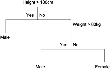
Example tree for classifying gender

FIGURE 2

Example tree to illustrate formulation with given

x

belonging to leaf 6

In practice, individual decision trees are often associated with high variance predictions and poor out‐of‐sample predictive accuracy. They will often overfit the data if they are not restricted in size (Breiman, 1996). Random forests decrease this variance using bagging. This involves taking the average of many trees, each trained by randomly sampling the training data and features that are used in the splits (Breiman, 2001). Random forests can be applied for either regression or classification problems.

Using a random forest as an objective function has many advantages. Random forests are a very powerful prediction algorithm which can fit unknown nonlinear and complex interactions of features with minimal feature engineering, making them popular and widely used in machine learning (Biau & Scornet, 2016). Furthermore, they are generally recognized as being able to deal effectively with high dimensional data and have few parameters to tune (Biau & Scornet, 2016). Of particular relevance to optimization, random forests have a special combinatorial structure which allows us to leverage the power of mixed‐integer linear programming and powerful existing solvers to solve large‐scale problems.

Contributions

First, we show how to solve optimization problems with random forest objective functions, with general polyhedral constraints. This allows us to model practical business considerations and restrict the policy to a particular function class. We show that it is possible to formulate this problem as a MIP, which can be further decomposed and solved iteratively using pareto‐optimal Benders cuts. Although the subproblems contain complicated binary logic, we provide a naturally integer subproblem formulation. This in turn allows us to consider the dual formulation and thus consider Benders cuts.

Second, we provide analytical guarantees on an approach that approximates a large‐scale random forest optimization problem by sampling and optimizing over a smaller forest. For axis‐aligned trees, we show that the number of trees we need to sample to be within ε of the optimal solution with probability
$1 - δ$
is sublinear in the size of the target forest. We achieve this by bounding the number of sets in a forest with axis‐aligned trees, and by showing, empirically, that this number is even smaller in many real‐world datasets. We also provide instances where this approach performs better than optimizing over trees with truncated depth.

Third, for very large problem instances, we propose heuristic algorithms that optimize over smaller forests using an approach inspired by cross‐validation. We derive analytical upper and lower bounds on the performance of the optimal solution from the heuristic.

Finally, we explore the performance of these algorithms using synthetic datasets as well as two original case studies with real data: a property investment and a jury selection case study. We show that our approaches outperform benchmarks optimizing other machine learning objective functions.

Our paper follows the following outline: in Section 3, we introduce the model, the MIP formulation, and show how to decompose this MIP using Benders decomposition and implement pareto‐optimal Benders cuts. In Section 4, we prove some analytical results about the suboptimality of a smaller random forest as an approximation to a large forest and introduce a heuristic based on cross‐validation for optimization. In Section 5, we introduce case studies on property investment and jury selection, respectively, and we explore the properties of the random forest algorithms on these datasets.

RELEVANT LITERATURE

Data‐driven optimization

There has been significant recent interest in incorporating machine learning techniques into data‐driven optimization problems. In particular, often machine learning is used to estimate the objective as a function of decisions and auxiliary covariates, which is called a “predict then optimize” approach. Bertsimas et al. (2016) use ridge regression in a data‐driven approach to design chemotherapy regimens for cancer. Baardman et al. (2019) use multiplicative regression (log‐linear) to estimate demand for promotion vehicles, which is used to maximize revenue. Besbes et al. (2010) optimize over a Nadaraya–Watson kernel regression function, where the kernel is Gaussian. Further examples of operations management problems incorporating covariate data into optimization problems include Ban et al. (2016); Ban & Rudin (2018); Aouad et al. (2019); Cohen et al. (2020); Bertsimas & Kallus (2020); Ban & Keskin (2021); Chen et al. (2021); Elmachtoub & Grigas (2022). There has recently been significant recent interest in modeling trained neural networks in this context using mixed‐integer optimization techniques (Anderson et al., 2020; Fischetti & Jo, 2018; Tjeng et al., 2017). We focus on modeling this relationship using tree ensembles.

There is some recent literature that incorporates random forests into a predict‐then‐optimize framework. Ferreira et al. (2015) study a pricing problem in retail, where prices come from a discrete ladder. They use a random forest to estimate the demand for the product conditioned on the price and make predictions for all price‐product combinations. This avoids having to optimize over the structure of the random forest, which would be necessary if the set of prices was significantly larger or continuous.

Since the initial version of this paper was released online, we became aware of Mišić (2020), who has simultaneously and independently studied optimizing tree‐based ensembles. The MIP formulation in Mišić (2020) is effective but is restricted to unconstrained problems or problems with box constraints on decision variables. In contrast, our model admits general polyhedral constraints. This provides flexibility for modeling a greater range of applications, and in particular, allows the policy class to be specified and modeled. Another significant difference is in heuristics used to solve large‐scale random forests. Mišić (2020) uses an approach that truncates trees at a certain depth, while we use an approach where we optimize over fewer trees and use cross‐validation procedure. We analyze the theory of optimizing over smaller forests and derive bounds on the suboptimality of doing so.

In the data mining community, there have been several papers studying sensitivity analysis for machine learning algorithms, in terms of the impact of an input of a predictive approach on its output. In particular, the inverse classification stream studies the problem of minimizing a probability of an event by finding the optimal set of actions (Aggarwal et al., 2010; Pendharkar, 2002). Some papers have introduced constraints in the optimization framework to enforce the solution's feasibility. These can be constraints that are imposed to eliminate extreme solutions (Barbella et al., 2009), to separate the contextual features from the decision features (Chi et al., 2012; Yang et al., 2012), or to limit the range of possible changes to the decision features (Lash & Zhao, 2016). However, when these constraints are considered altogether, nondifferentiable classifiers are underexplored. In contrast, our MIP formulation offers a more flexible framework with a wider class of constraints to optimize a random forest output (which is nonconvex and nondifferentiable). Furthermore, to solve this problem, these papers use heuristic‐based methods such as variable neighborhood search (VNS), genetic algorithms, and hill‐climbing leading to locally optimal solutions. In our work, we can solve the MIP formulation globally optimally as well as improve the speed of the MIP solver by introducing Benders cuts.

There have been recent efforts to apply modern optimization techniques to estimate globally optimal classification trees, rather than by following a greedy estimation heuristic as has been done in CART. Bertsimas and Dunn (2017) present a mixed‐integer linear programming (MIP) formulation and show it outperforms widely used heuristics for datasets of a reasonable size. They focus on training trees (optimal estimation), whereas our optimization is focused on choosing the best “input feature vector” given an ensemble of trees.

Relation to causal inference

In the causal inference literature, the approach of estimating a model from data, and then using this model to estimate the reward of a policy is often broadly referred to as a direct method or direct comparison approach (Qian & Murphy, 2011). Our approach falls within this class of problems but focuses on the difficulty of solving the resulting optimization problem when the model is a tree ensemble model and the decision is complex (multi‐dimensional and/or constrained), so a simple enumeration or search for the optimal policy is not tractable. As such, we are agnostic to the estimation procedure used to train the tree ensemble, and indeed, our approach can be adapted to optimize tree ensembles trained using different techniques, as would be appropriate under different assumptions on the data.

The success of direct comparison methods depends on whether the fitted model is a good representation of the relationship between outcome, decision, and scenario data. A prerequisite for this is to have appropriate data. One key assumption made in direct comparison methods is unconfoundedness. This requires measurement of the right covariates to separate the effect of the treatment itself from the effect of the assignment. More precisely, under the potential outcomes framework, where we observe the action
$Z_{i}$
, the outcome for that action
$Y_{i}$
, and covariates
$W_{i}$
for a sample but do not observe the counterfactual outcome
$Y_{i} (z)$
if some other action z had been taken, the assumption is that
$Y (z) ⊥ ⊥ Z | W$
. This means that the outcome is independent from the decision conditioned on the observed covariates. Under this assumption,
$E [Y (z) | W] = E [Y | W, Z = z]$
(Kallus, 2017). If the fitted model is close to the conditional expected value, a standard random forest model can be expected to work well. For example, in an ideal setting of a randomized trial, where the decision/treatment is applied randomly to the population of interest, using a standard random forest can find optimal personalized policies.

If the unconfoundedness assumption is not satisfied, in particular, if there are hidden confounding variables that affect both the observed decision and the outcome, then different techniques need to be used, such as instrumental variables. These can be incorporated into a random forest approach (Athey et al., 2019). We can also adapt other tree ensemble methods from the causal inference literature, such as causal random forests (Wager & Athey, 2017). These are intended for estimating individual treatment effects with binary treatments, so they cannot be directly plugged into our framework, but the core idea of using honest trees (Athey & Imbens, 2016) is applicable to our setting. Honest trees incorporate a sample splitting procedure so that different data are used to construct the tree (a sequence of variables splits), to the data used to estimate the outcomes in each leaf. This generally improves estimates in each leaf as they are no longer correlated with the tree construction. Causal forests also require the unconfoundedness assumption. There is a variety of different causal inference methods which are suitable for different data settings. Many of these approaches involve estimation using tree ensembles, and as long as they give estimates of the reward given the decision and outcome, our method can be used to solve the corresponding optimization problem.

MODEL

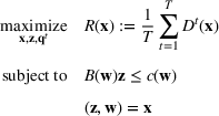
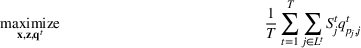
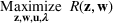
Our goal is to maximize
$R (z, w)$
, where
$z$
is a decision,
$w$
is a scenario represented by covariate data, and
$R (z, w)$
is the predicted outcome from a trained random forest model. Our decision variables lie in some feasible polyhedral set
${(z, w) | B (w) z \leq c (w)}$
, potentially depending on the scenario. Concrete examples of data‐driven optimization problems with decisions, outcomes, and scenario‐dependent polyhedral sets are given in Sections 5.1 and 5.2. For notational convenience, we introduce
$x = (z, w)$
.

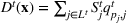
The random forest is the average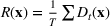
$R (x) = \frac{1}{T} \sum D_{t} (x)$
, where
$D_{t} (x)$
is the predicted outcome from that a single tree t and T is the number of trees in the random forest. A decision tree iteratively partitions the space of
$x$
, by branching on conditions relating to those features. If
$a_{i t}^{'} x \geq b_{i}^{t}$
, then we move to the right child node of i in the tree; otherwise, we move to the left child node of i. In most commonly used implementations of random forests, splits are axis‐aligned, such that only one dimension of x is involved in the split,
$x_{j} \geq b_{i}^{t}$
. After a number of splits, we arrive at a leaf, which is a set of
$x$
that share the same score.

We introduce the following notations for our model: For every tree
$t \in [T]$
, denote
$N^{t}$
the set of interior nodes (not leaves) in tree t. Specifically,
$N_{r}^{t}$
(respectively
$N_{l}^{t}$
) is the set of interior right nodes (respectively left nodes). Let
$L^{t}$
be the set of leaves in tree t. Specifically,
$L_{r}^{t}$
(respectively
$L_{l}^{t}$
) is the set of right leaves (respectively left leaves). For every node
$i \in N^{t}$
,
$p_{i}$
,
$l_{i}$
and
$r_{i}$
are the immediate parent, the left child, and the right child of node i.
$S_{j}^{t}$
is the score of each leaf
$j \in L^{t}$
. We introduce binary variables to track which leaf a solution
$x$
belongs to, according to the branches of the tree. For every node i and
$j \in {r_{i}, l_{i}}$
,
$q_{i, j}^{t}$
is a binary variable such that
$q_{i, j}^{t} = 1$
if and only if the solution
$x$
is in a leaf that is a descendant of node j. This notation is illustrated in Figure 2 which gives an example of how variables are set for a given tree. In view of the introduced notation, we can write
$D^{t} (x) = \sum_{j \in L^{t}} S_{j}^{t} q_{p_{j}, j}^{t}$
as the score of a tree and thus our problem is to maximize:
$\begin{matrix} \underset{x, z, q^{t}}{maximize} & R (x) : = \frac{1}{T} \sum_{t = 1}^{T} D^{t} (x) \\ subject to & B (w) z \leq c (w) \\ (z, w) = x \end{matrix}$
2In other words, this objective is to maximize the average of the scores of the leaves that are active because the solution
$x$
lies within the leaf. In the following, we will present a MIP formulation that encodes the tree dynamics.

MIP formulation

We need logical constraints which determine which leaf a solution
$x$
lies in. If at an interior node i in tree t we move to the right child of i, that is,
$a_{i, t}^{'} x \geq b_{i}^{t}$
, we force the MIP to only consider the leaves that are a descendant of right child of node i, by setting
$q_{i, l_{i}}^{t}$
to 0. Likewise, if
$a_{i, t}^{'} x \leq b_{i}^{t}$
, we set
$q_{i, r_{i}}^{t}$
to 0. These two logical constraints can be modeled using the big‐M method :
$\begin{matrix} a_{i, t}^{'} x - M (1 - q_{i, l_{i}}^{t}) \leq b_{i}^{t}, and a_{i, t}^{'} x + M (1 - q_{i, r_{i}}^{t}) \geq b_{i}^{t} . \end{matrix}$
3This assumes that
$x$
is bounded, so that
${\underset{̲}{x}}_{i} \leq x_{i} \leq {\bar{x}}_{i}$
for some
${\underset{̲}{x}}_{i} \leq {\bar{x}}_{i}$
. If the splits are axis‐aligned, as is the case for Breiman's original random forest, we can replace M with
$\max {| {\underset{̲}{x}}_{j} |, | {\bar{x}}_{j} |} + b_{i}^{t}$
. Similarly for oblique splits, we replace M by
$\max_{\underset{̲}{x} \leq x \leq \bar{x}} a_{i, t}^{'} x + b_{i}^{t}$
. We can now write the following MIP formulation (P):
$\begin{matrix} \underset{x, z, q^{t}}{maximize} & \frac{1}{T} \sum_{t = 1}^{T} \sum_{j \in L^{t}} S_{j}^{t} q_{p_{j}, j}^{t} \end{matrix}$
P
$\begin{matrix} subject to & a_{i, t}^{'} x - M (1 - q_{i, l_{i}}^{t}) \leq b_{i}^{t}, \forall t \in [T], i \in N^{t} \end{matrix}$
4
$\begin{matrix} a_{i, t}^{'} x + M (1 - q_{i, r_{i}}^{t}) \geq b_{i}^{t}, \forall t \in [T], i \in N^{t} \end{matrix}$
5
$\begin{matrix} q_{i, r_{i}}^{t} + q_{i, l_{i}}^{t} = q_{p_{i}, i}^{t}, \forall t \in [T], i \in N^{t} \end{matrix}$
6
$\begin{matrix} \sum_{i \in L^{t}} q_{p_{i}, i}^{t} = 1, \forall t \in [T] \end{matrix}$
7
$\begin{matrix} q_{i, l_{i}}^{t}, q_{i, r_{i}}^{t}, q_{p_{i}, i}^{t} \in {0, 1}, \forall t \in [T], i \in N^{t} \end{matrix}$
8
$\begin{matrix} B (w) z \leq c (w) \end{matrix}$
9
$\begin{matrix} (z, w) = x \end{matrix}$
10Constraint (6) enforces that if a parent node is not active, then the children will not be active either, but if a child is active then the parent is active too. Constraint (7) enforces that for each tree t, there is only one leaf that is active. Constraints (4)–(8) are sufficient to uniquely determine the active leaf for a given solution
$x$
for every tree. Constraint (9) is the (possibly scenario dependent) problem‐specific feasible set for our decision, while constraint (10) is for ease of notation.

Alternative MIP formulations for trees are possible, such as the union of polyhedra formulation of Biggs and Perakis (2019). However, it is shown in that article that the numerical performance is generally not superior to the big‐M formulation presented in this article in the case of modeling tree ensemble objectives. In addition to that, it does not allow for Benders decomposition (Section 3.2), which greatly improves its performance. Furthermore, the formulation of Mišić (2020) cannot be applied to this setting with general polyhedral constraints without introducing considerable complexity.

Another powerful tree ensemble method which often has a higher predictive accuracy than random forests is gradient‐boosted trees, including AdaBoost (Freund & Schapire, 1997), XGBoost (Chen & Guestrin, 2016), and LightGBM (Ke et al., 2017) approaches. Gradient‐boosted trees iteratively fit new trees to the residuals of the previous ensemble model, therefore, improving in model accuracy (at least on the training set) with subsequent rounds. The final model is a weighted sum of trees
$\frac{1}{T} \sum_{t} γ_{t} D_{t}^{'} (x)$
. We can easily adapt our MIP formulation and Benders decomposition approach to model these trees by setting
$S_{i}^{t} = γ_{t} S_{i}^{t^{'}}$
, where
$S_{i}^{t^{'}}$
is the score and
$γ_{t}$
is the weight associated with the boosting round t.

Benders decomposition

The previous formulation can be slow to solve to optimality for large problem instances, as explored in Section 5.3. Fortunately, this problem has a structure that makes it an attractive candidate for Benders decomposition with lazy constraint generation. The problem can be decomposed into the master problem (MP) that chooses a solution
$x$
, and T subproblems that find the variables which determine the score of the leaf for each tree t for a given solution
$x$
. One requirement for Benders decomposition to provide an improvement is that the subproblem solves quickly. We show that if we introduce additional variables and reformulate the problem (P), the resulting subproblem is naturally integer. By strong duality, we reformulate the linear primal subproblem and generate constraints iteratively using Benders cuts. We present the related mixed‐integer formulation and the algorithm‐generating Benders cuts in Section S1.1.

To generate Benders cuts, we can solve the dual linear problem to retrieve the dual solution. However, This can be time‐consuming for large problem instances, since we need to solve an LP to generate a cut every time. Due to the special structure of the dual problem, we can find an explicit analytical expression of a viable solution to the dual solution. We provide the expression of the analytical solution in Section S1.2.

Using Benders cuts results in a significant speed improvement because we only generate cuts for the objective as required. This improvement is explored numerically in Section 5.3. An issue with our dual subproblem is degeneracy. There are often multiple optimal dual solutions. Pareto‐optimal cuts have been implemented in many applications employing Benders decomposition (Mercier et al., 2005; Santoso et al., 2005), and in the work conducted by Magnanti and Wong (1981) and Tang et al. (2013), it has been shown that their use can speed up the convergence of the algorithm.¹ Magnanti and Wong (1981) propose a method to generate pareto‐optimal cuts when the objective of the subproblem dual is linear with the variable vector
$x$
. In Section S1.3, we show in detail how we generate pareto‐optimal cuts in our particular setting where the subproblem is nonlinear with
$x$
(but still linear with respect to the auxiliary variable vector g). This is necessary to apply Benders decomposition in our setting.

APPROXIMATING LARGE RANDOM FORESTS

Analytical results

While the MIP formulation can solve many real‐world datasets to optimality in a reasonable amount of time, for large‐scale data, the MIP can be prohibitively slow. Motivated by this, we explore a sampling heuristic that is faster while still obtaining good solutions. Suppose we have a large target forest
$R_{T}$
with T trees that we would like to use as our ideal objective function. Instead of optimizing this large forest, we propose randomly sampling the trees which make up the target forest and optimizing over a smaller, sampled forest. In this section, we will analyze how the quality of this solution changes with the size of the sampled forest.

We can consider the random forest to be a partition of the feature space into m disjoint sets indexed by
$i \in [m]$
. This restricts the search for the optimal feature vector to m different feature vector regions. Suppose we look at the scores of a forest
$R_{n}$
composed of a random sample of n trees. Denote
$X_{i}^{t}$
to be the score of a sampled tree t for set i, and let
$Y_{i} = \frac{1}{n} \sum_{t = 1}^{n} X_{i}^{t}$
be the score of the sampled forest for set i. We note that
$X_{i}^{t}$
and
$Y_{i}$
are random variables because they depend on which trees are sampled. Let
$s_{i}$
be the score of set i in the target random forest such that
$Y_{i}$
is a noisy estimate of the score
$s_{i}$
, and
$E [X_{i}^{t}] = E [Y_{i}] = s_{i}$
.

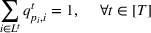
The only assumption we make is that the scores between trees for the same set are independent and identically distributed (i.i.d.), that is, for any pair of trees
$t_{1}, t_{2}$
and set i,
$X_{i}^{t_{1}}$
and
$X_{i}^{t_{2}}$
are i.i.d. This assumption is justified since the trees are sampled independently with replacement from the target random forest. This assumption is also satisfied when creating trees in Breiman's original algorithm as long as we condition on the training data, due to the random variables defining data sampling, feature sampling, and split generation being independent. We allow the scores of sets in a partition within the same tree to have an arbitrary dependence structure.

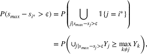
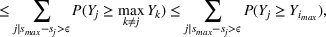
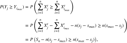
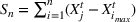
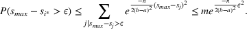
If we optimize over the sample random forest, the set to which the chosen solution belongs is
$i^{} = {arg max}_{i} {Y_{i}}_{i = 1}^{m}$
. The optimal set
$i^{}$
is also a random variable because the set we choose in the sampled forest will depend on which trees are sampled. However, we are interested in the score of this solution as evaluated on the target random forest, as this is our best estimate of the performance of the solution. We can quantify the suboptimality of our solution by calculating
$s_{m a x} - s_{i^{}}$
, where
$s_{m a x}$
is the optimal objective of the target random forest:
$s_{m a x} = \max_{i} {s_{i}}_{i = 1}^{m}$
. We note that in practice we are optimizing over a subset of the m sets since not all sets in the random forest are necessarily feasible for a given scenario in an optimization problem. For example, if
$w$
is fixed, then we are restricted to leaves that contain
$w$
. As such, m is an upper bound on the number of sets. However, for simplicity, we omit this dependence from our notation. We next present a result which shows how the probability of the proposed solution being suboptimal decays as we increase the size of the sampled random forest n. Theorem 1
Let
$X_{i}^{t}$
be random variables, independent with respect to t, that lie in the interval
$[a, b]$
, with
$E [X_{i}^{t}] = s_{i} \forall t \in [T], i \in [m]$
. Let
$Y_{i} = \frac{1}{n} \sum_{t = 1}^{n} X_{i}^{t}$
and
$i^{} = {arg max}_{i} {Y_{i}}_{i = 1}^{m}$
, while
$s_{m a x} = \max_{i} {s_{i}}_{i = 1}^{m}$
. Let
$δ \in (0, 1)$
. Then with probability at least
$1 - δ$
:
$s_{m a x} - s_{i^{}} \leq \sqrt{2} (b - a) \sqrt{\frac{l o g (m) + l o g (1 / δ)}{n}} .$
11In other words, to guarantee
$s_{m a x} - s_{i^{}} \leq ε$
with probability at least
$1 - δ$
, the amount of trees sampled should be
$n \geq Ω (\frac{l o g (m) + l o g (1 / δ)}{ε^{2}}) .$
12

Proof of Theorem 1
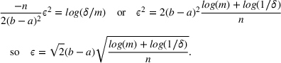
We previously defined
$s_{m a x} = \max_{i} {s_{i}}_{i = 1}^{m}$
. Denote the set index
$i_{m a x}$
such that
$s_{m a x} = s_{i_{m a x}}$
. We have:
$\begin{matrix} P (s_{m a x} - s_{i^{}} > ε) & = P (⋃_{j | s_{m a x} - s_{j} > ε} 1 {j = i^{}}) \\ = P (\cup_{j | s_{m a x} - s_{j} > ε} Y_{j} \geq \max_{k \neq j} Y_{k}), \end{matrix}$
13
$\begin{matrix} \leq \sum_{j | s_{m a x} - s_{j} > ε} P (Y_{j} \geq \max_{k \neq j} Y_{k}) \leq \sum_{j | s_{m a x} - s_{j} > ε} P (Y_{j} \geq Y_{i_{m a x}}), \end{matrix}$
14where the second equality results from the definition of
$i^{}$
and the first inequality is a result of the probability union bound. We can then rewrite
$P (Y_{j} \geq Y_{i_{m a x}})$
as the following:
$\begin{matrix} P (Y_{j} \geq Y_{i_{m a x}}) & = & P (\sum_{i = 1}^{n} X_{j}^{t} \geq \sum_{i = 1}^{n} X_{i_{m a x}}^{t}) \\ = & P (\sum_{i = 1}^{n} X_{j}^{t} - \sum_{i = 1}^{n} X_{i_{m a x}}^{t} - n (s_{j} - s_{m a x}) \geq n (s_{m a x} - s_{j})) \\ = & P (S_{n} - n (s_{j} - s_{m a x}) \geq n (s_{m a x} - s_{j})), \end{matrix}$
15where we denote
$S_{n} = \sum_{i = 1}^{n} (X_{j}^{t} - X_{i_{m a x}}^{t})$
. We have
$E [S_{n}] = n (s_{j} - s_{m a x}) < - n ε < 0$
for all
$j \in {k | s_{m a x} - s_{k} > ε}$
. Furthermore,
${X_{j}^{t} - X_{k}^{t}}_{t = 1}^{n}$
are iid and bounded by
$[n (a - b), n (b - a)]$
. Using Hoeffding's inequality, it follows that:
$\begin{matrix} P (S_{n} - n (s_{j} - s_{m a x}) \geq n (s_{m a x} - s_{j})) \leq e^{\frac{- 2 n^{2} {(s_{m a x} - s_{j})}^{2}}{n {(2 b - 2 a)}^{2}}} \leq e^{\frac{- n {(s_{m a x} - s_{j})}^{2}}{2 {(b - a)}^{2}}} . \end{matrix}$
16It follows from inequalities (17) and (14) that
$P (s_{m a x} - s_{i^{}} > ε) \leq \sum_{j | s_{m a x} - s_{j} > ε} e^{\frac{- n}{2 {(b - a)}^{2}} {(s_{m a x} - s_{j})}^{2}} \leq m e^{\frac{- n}{2 {(b - a)}^{2}} ε^{2}} .$
17

Setting the right hand side bound equal to δ and solving for ε, we have:
$\begin{matrix} \frac{- n}{2 {(b - a)}^{2}} ε^{2} = l o g (δ / m) or ε^{2} = 2 {(b - a)}^{2} \frac{l o g (m) + l o g (1 / δ)}{n} \\ so ε = \sqrt{2} (b - a) \sqrt{\frac{l o g (m) + l o g (1 / δ)}{n}} . \end{matrix}$
18

That is, with probability at least
$1 - δ$
, we have:
$s_{m a x} - s_{i^{}} \leq \sqrt{2} (b - a) \sqrt{\frac{l o g (m) + l o g (1 / δ)}{n}} .$
19

$□$

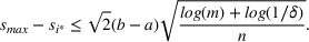
Theorem 1 allows us to bound the suboptimality of the sampled solution by
$O (\sqrt{l o g (m) / n})$
with probability at least
$1 - δ$
. In particular, as long as the number of sets m does not scale exponentially with the number of trees in the target random forest T, the accuracy will converge to 0 with a sublinear rate.

A relevant result to Theorem 1 can be found in Kleywegt et al. (2002) where the authors bound the suboptimality of the SAA approximation of stochastic discrete optimization using Cramér's large deviation (LD) theorem. Similar to our use of Hoeffding's inequality, the LD theory can be used to derive exponential bounds on tail distributions of sums of independent random variables. However, estimating the theoretical bounds in Kleywegt et al. (2002) is not a straightforward task, and thus can complicate the practical use of the SAA approximation method. 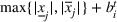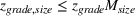Instead, the bound in Theorem 1 only uses the number of sets in the random forest m and the bounds on the set scores a and b. Finally, Kleywegt et al. (2002) considers a setting with a finite discrete feasible set and the size of the feasible set impacts their theoretical error bounds. The authors mention that it can potentially grow exponentially with the problem input parameters, but a deep analysis of this behavior and how it impacts their results is beyond the scope of their paper. In contrast, we provide this analysis for the random forest setting. In particular, due to the importance of m in the bound in Theorem 1, we examine how large m is for a given target forest of T trees.

For this analysis, we focus on axis‐aligned splits, which are implemented in the most widely used tree ensemble methods. These are splits of the form
$x_{i} \leq b_{j}$
, where each split only occurs on one dimension
$x_{i}$
. The number of splits is equal to the number of interior nodes in the forest. In this setting, the number of sets m is limited because the axis‐aligned hyper‐planes can only intersect each other a limited number of times. In particular, in the worst case, the number of sets m in the random forest scales polynomially with the number of trees in the forest T, where the polynomial's degree is d (the dimension of the feature space). This is proved in the following Lemma. Lemma 1
For a random forest with T trees and at most
$h_{m a x}$
axis‐aligned splits per tree and feature space
$X^{d}$
, the number of sets m is polynomial in T with degree d:
$m \leq {(\frac{T h_{m a x} + d}{d})}^{d}$
20

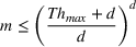
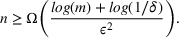
The proof can be found in S2. A similar bound can be derived from the known result that arranging n hyperplanes in d‐dimeniosnal space can cut the space into upto
$\sum_{i = 0}^{d} (\binom{n}{i})$
regions, which is also
$O (T^{d})$
. We now have the following corollary which incorporates the size of m from Lemma 1. Corollary 1
In the setting of Theorem 1, if the target random forest has axis‐aligned splits and feature space dimension d, then to guarantee
$s_{m a x} - s_{i^{}} \leq ε$
with probability at least
$1 - δ$
, the amount of trees sampled should be
$n \geq Ω (\frac{d \cdot l o g (T \frac{h_{m a x}}{d} + 1) + l o g (1 / δ)}{ε^{2}}) .$
21

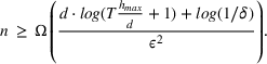
This corollary provides guidance on how to select the number of trees in the sampled random forest to obtain a desired accuracy level. In particular, it suggests choosing n larger than
$Ω (l o g (T))$
, which can result in a significant reduction in solve time, as it is exponential in the number of trees due to the complexity of optimizing the MIP formulation. Furthermore, to prevent overfitting, often
$h_{m a x}$
is relatively small and can be chosen by tuning the complexity parameter, depth of the tree, or minimum sample size per leaf during tree construction. Also, in our setting, the sum of the decision and covariate dimension is
$d = d_{z} + d_{w}$
. The covariate dimension
$d_{w}$
can be made smaller by dimensionality reduction or feature importance selection, although care needs to be taken to avoid potential confounding issues.

Also, it is worth noting that Lemma 1 provides an upper bound on the actual number of sets m, while in practice m is likely to be much smaller than that bound. This is because we often make decisions that are conditional on the scenario/covariate data
$w$
. In this case, there is only a much smaller subset of leaves/sets where our decision can fall. Furthermore, each tree only has at most
$h_{m a x} + 1$
sets, due to each split in the tree splitting an existing set in two, therefore creating one additional set. The proof above assumes that each axis‐aligned split can intersect all splits from each dimension which often does not occur for each tree. This is explored in the next section, where we numerically analyze several sets that are formed in random forests on real‐world datasets, suggesting the subset selection approach is stronger than stipulated in Corollary 1.

Number of sets in a random forest: a simulation study

We have shown that for trees with axis‐aligned splits, m is at worst polynomial in T, with degree d. However, in practice, the scaling is often not as severe as this worst‐case scenario. We provide experimental evidence to show that in many real‐world datasets, m scales with T according to a low order polynomial, and often the scaling is even linear or sublinear.

We provide the following experimental setup to explore this relationship. The number of nonempty sets m in a given random forest is difficult to calculate in an exact manner. As a proxy, we set up a uniform grid over the feature space and evaluate the random forest at each point. To approximately estimate the number of sets, we count the number of points in the grid which have a unique score. If the grid is sufficiently fine, this is likely to be a good approximation. The number of data points to form a grid of fixed resolution is exponential in the dimension. For tractable experiments, we fix the number of points in the grid at 10,000,000, and use a lower resolution for the higher dimension tests. While this approach is most effective for low dimension datasets as the grid is the most dense, we tractably test datasets of dimension 1–5, by scaling the number of data points per dimension by
$10, 000, 000^{\frac{1}{d}}$
. For example, for
$d = 2$
, we use a grid which is 3162 × 3162.

We evaluate the approximate number of sets on datasets which have been used in the context of optimizing tree ensembles. In particular we evaluate on wine (Cortez et al., 2009), solubility (Huuskonen, 2000), concrete (Yeh, 1998) from Mišić (2020), and housing (Harlfoxem, 2016) described in detail in Section 5.1. These datasets have size of
$n = 1599, 951, 1030, 21614$
, and dimension
$d = 11, 228, 8, 19$
, respectively. We repeat experiments for each dataset increasing dimension from 1 − 5 according to feature relevance. We count the number of unique sets for forests with increasing number of trees
${1, 2, 4, 8, 16, 32, 64}$
. All forests are trained using default settings from Scikit‐learn RandomForestClassifier.

To evaluate the scaling between number of sets and number of trees, we fit different regression models to see which best fit this relationship empirically. In particular, we fit the following models: (i) linear
$m = θ_{1} T + θ_{0}$
, (ii) exponential
$m = θ_{0} e^{θ_{1} T}$
, and (iii) multiplicative
$m = θ_{0} T^{θ_{1}}$
.

We report the R ² of each model to evaluate which model best captures the relationship between the number of sets and the number of trees. A stronger R ² suggests the model is more suitable for the scaling. This can be observed in Table 2. We also report on θ₁ from the multiplicative model. This represents the approximate degree of a model which is polynomial in T. In particular, if
$θ_{1} \approx 1$
, this suggests the scaling is approximately linear, while if
$θ_{1} \leq 1$
, this suggests the scaling is sublinear. This can be observed in Table 3.

TABLE 2
R ² of regression models describing relationship between number of sets and number of trees

Dimension

Dataset Model 1 2 3 4 5

house Linear 0.55 0.83 0.98 0.99 0.99

Exponential 0.55 0.73 0.69 0.58 0.55

Multiplicative 0.93 0.99 0.98 0.99 0.91

solubility Linear 0.67 0.74 0.53 0.72 0.72

Exponential 0.59 0.60 0.51 0.61 0.58

Multiplicative 0.91 0.88 0.90 0.94 0.90

wine Linear −0.40 0.99 0.99 1.00 1.00

Exponential −0.15 0.62 0.65 0.76 0.77

Multiplicative 0.73 0.93 0.98 1.00 1.00

concrete Linear 0.58 1.00 0.99 0.99 0.99

Exponential 0.55 0.53 0.41 0.40 0.36

Multiplicative 0.90 0.85 0.79 0.79 0.72

Plots of the relationship between the number of sets, the number of trees, and the dimension can be found in Figure 3. Overall, we observe that for these datasets, the number of sets with unique scores often scales sublinearly with the number of trees in the forest. This can be observed in particular for house and solubility datasets. Furthermore, Table 3 shows that the degree of polynomial which best describes the relationship between the number of trees and number of sets is often less than 1, showing that it is often sublinear. The highest degree in all experiments is 2.07, which is still relatively low.

FIGURE 3
How the number of sets scales with the number of trees. Rows: housing, solubility, wine, and concrete datasets. Columns: Dimension
$d = 1, 3, 5$

Furthermore, Table 2 shows that the exponential model never fits as well as the linear or multiplicative models, suggesting that the true relationship between the number of sets and the number of trees is unlikely to be exponential. While these experiments are imperfect and are less reliable for large d, this evidence combines to suggest that the bounds from Theorem 1 will be relatively strong in practice, as these simulations show that m does not scale adversely with T. Also in line with these results, we observe promising performance for forests even with a small number of trees in Section 5.3.4. This motivates us to explore heuristics limiting the number of trees since we get diminishing returns on adding trees to the random forest when it is large, but the solve time is exponential in the number of trees due to the MIP formulation.

TABLE 3
Degree of polynomial θ₁ for best regression model describing relationship between number of sets and number of trees

Dimension

Dataset 1 2 3 4 5

house 0.28 0.39 0.91 1.43 1.38

solubility 0.46 0.63 0.37 0.43 0.58

wine 0.14 1.19 1.30 0.92 0.91

concrete 0.39 1.53 1.93 1.98 2.07

Cross‐validation for optimization

Following the previous section, we propose a heuristic where we decompose a large target random forest into several smaller random forests. For each random forest subset, we select the optimal solution using our MIP formulation. We then test each solution against the forests it was not optimized over, to get the average score referred to from now on as the out‐of‐forest score. We then pick the solution which has the best out‐of‐forest score. The rationale behind this heuristic is that we can solve many smaller MIPs much faster than we can solve one large MIP. Furthermore, we can pick a solution that is robust relative to different forests, mitigating the effects of overfitting due to using a limited number of trees in the optimization. We describe the procedure below more formally (Algorithm 1):

ALGORITHM 1
Cross‐validation for optimization

1: Train τ forests $R_{1} (\cdot), …, R_{τ} (\cdot)$ on the data

2: Find optimal solution for each forest
$x_{i} = {arg max}_{x \in X} R_{i} (x) \forall i \in [τ]$

3: Calculate
$\bar{R} (x_{i}) = \frac{1}{τ} \sum_{j} R_{j} (x_{i}) \forall i \in [τ]$

4: Pick
$x^{C V} = {arg max}_{i \in [τ]} \bar{R} (x_{i})$

We can derive analytical bounds on the performance of this algorithm. Due to a random forest being the average of several trees (or equivalently average of smaller random forest), the global optimal solution is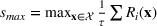
$s_{m a x} = \max_{x \in X} \frac{1}{τ} \sum R_{i} (x)$
. Proposition 1
Let
$x^{C V}$
be the solution derived from the cross‐validation for optimization procedure over τ forests
$R_{1}, …, R_{τ}$
. Then,
$\frac{1}{τ} \sum_{i = 1}^{τ} R_{i} (x^{C V}) \leq s_{m a x} \leq \frac{1}{τ} \sum_{i = 1}^{τ} \max_{x \in X} R_{i} (x)$
.

The proof can be found in Section S2. These bounds are very useful in practice; if we solve the heuristic for forests of a certain size, we know how good the obtained solution is relative to the best solution, and how much we could potentially gain by repeating the heuristic with larger forests. This allows the practitioner to make an informed decision about whether to increase the forest size with consideration of the computational burden.

Although it is straightforward to adapt the MIP techniques in this article to boosted trees, the sampling and cross‐validation approaches we provide are not suitable to apply to boosted trees algorithms. There are two issues: First, since in each boosting round the new tree is fitted to the residuals of the existing tree ensemble, the score of each leaf in a tree
$X_{i}^{t}$
will in general not be independent across trees. Second, due to this residual fitting process, each tree is unlikely to be a good estimate of the outcome if the tree ensemble that was fitted in the previous rounds is not included in its entirety. A sampling process that randomly omits trees is unlikely to work well for this reason. A more sensible heuristic to use when optimizing boosted tree ensembles is to batch optimize in the order of the boosting rounds, using the first k ₁ trees, solve to optimality, then introduce the next k ₂ and solve using the previous solution as a warm start, repeating until the desired precision is achieved.

NUMERICAL EXPERIMENTS

We now describe in detail two case studies with real data which both analyze the behavior of the algorithms we have introduced and explore the effectiveness of a random forest compared to optimizing over different objective functions. These case studies are both constrained optimization problems, which cannot be easily solved using unconstrained formulations (such as in Mišić, 2020).

Case study: Property investment

Property investors face difficulty in assessing how much a property will sell for on the market. Residential properties have many different features (such as the number of bedrooms, bathrooms, floors, size of the house, quality of construction, and location), which are prioritized and valued in different ways by different buyers. Furthermore, there is a degree of unpredictability in the sale price depending on which buyers happen to be interested in a property. This makes it hard for property investors to make sound investment decisions when evaluating the different options available. In particular, we look at a situation in which the property investor is interested in buying an empty lot, constructing a new house, and then selling that property to make a profit. We overcome this uncertainty by estimating the sale price for a given property using a random forest model trained from data on previous house sales. We then optimize to find the property which is predicted to achieve the highest price, as predicted by the random forest.

Prediction

We have data from Kaggle on house sale prices for King County, which includes Seattle (Harlfoxem, 2016). It includes 21,613 houses sold between May 2014 and May 2015. We divide the features into those related to the house and those related to the lot as shown in Table 4. Table 5 shows the performance of various algorithms for predicting the sale price of a property. We used a 70% / 30% training / testing split. We see that XGBoost (another ensemble tree approach) performs the best with 90% OOS accuracy while Random Forest performs second best with 88% OOS accuracy. Regression approaches do worse, achieving around 70% OOS accuracy (Table 5).

TABLE 4
Variables of housing dataset

House variables Meaning Lot variables Meaning

bedrooms Number of bedrooms zipcode Zipcode house is located in

bathrooms Number of bathrooms lat Latitude of house

size Square footage of the home lon Longitude of house

base Square footage of the basement sqftlot Square footage of the lot

grade Quality of construction water View of waterfront (binary)

TABLE 5
Predictive accuracy house sales prices

Model Training accuracy (R ²) Testing accuracy (R ²)

Random forest 98 88

XGBoost 100 90

CART 99 76

Ridge regression 70 70

Linear regression (OLS) 70 69

TABLE 6
Variables of jury dataset

Jury variables Meaning Case variables Meaning

police Trust the police deftgend Defendant's gender

amcourts Trust the courts defrace Defendant's race

crmsevre Think crime serious problem victgend Victim's gender

previous Been a juror before victrace Victim's race

civilcrm Previous jury‐criminal of civil victrela Victim's relationship to defendant

gender Gender casetype Case type

age Age

school Highest level of education

race Race/ethnicity

religion Strength of religious beliefs

income Household income

jobstat Job status

occupat Occupation

TABLE 7
Predictive jury verdict averaged over 20 data splits

Model Training accuracy (%) Testing accuracy (%)

Random forest 59 60

XGBoost 100 57

CART 85 51

SVM 53 53

Logistic regression 65 56

Linear regression 53 49

Random forest with only case features (baseline) 55 54

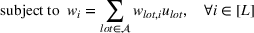
Formulation

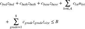
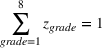
Suppose we have a number of empty sections the investor has to choose between. The investor needs to decide (i) which lot to purchase and (ii) what kind of house to build on that lot. We assume the property investor has a fixed budget with which to buy the lot and construct the house. The property investor wants to maximize the sale price (or predicted value) of the resulting house.

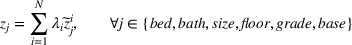
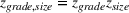
Suppose we have trained a random forest
$R (z, w)$
from data to predict the property sale price, where
$z = (z_{b e d}, z_{b a t h}, z_{s i z e}, z_{g r a d e}, z_{b a s e})$
are the features of the house, while
$w = (w_{z i p}, w_{l a t}, w_{l o n}, w_{s q f t l o t}, w_{w a t e r})$
are the features of the lot, corresponding to Table 4. We want to maximize the sale price by maximizing
$R (z, w)$
as our objective, with
$z$
as our decision variable. We assume that
$R (\cdot, \cdot)$
has been trained a priori on a housing dataset and is treated as an input for the optimization model. We have
$z_{b e d}, z_{b a t h} \in Z^{+}$
,
$z_{s i z e}, z_{b a s e}, \in R^{+}$
and a binary vector
$z_{g r a d e} \in {0, 1}^{8}$
denoting which grade of materials the house is built out of.

Suppose there is a set
$A$
of available lots the property investor has to choose from. Each lot l has a vector of features
$w$
which describes the lot (size, zip code, etc—see Table 4). Let L be the number of features of the lot. Define
$u_{l o t}$
as a binary variable, with
$u_{l o t} = 1$
if we choose lot l, 0 otherwise. Constraint (23) assigns the features of the chosen lot to the vector
$w$
. Constraint (24) specifies that only one lot is chosen.

Let
$c_{l o t}$
be the cost of purchasing a lot,
$c_{b a t h}$
and
$c_{b e d}$
be the cost of building each bathroom and bedroom, respectively. Let
$c_{b a s e}$
be the cost per square foot of constructing a basement, and
$c_{g r a d e}$
be the cost per square foot of constructing a house with a given quality grade. Constraint (25) requires that the cost of purchasing the lot and constructing the house is less than a given budget B. We have an additional constraint (26) requiring that the size of the house is smaller than the size of the lot.

We also require the house chosen to be within the convex hull of the set of properties observed in the data. This ensures the feasible set is bounded, and that the selected house is not too dissimilar from the houses observed in the dataset. Let
${{\tilde{z}}^{i}}_{i = 1}^{N}$
be the features of the N houses in the dataset the random forest was trained on. This restriction is enforced in constraint (28) and (29). Although this introduces N additional variables
$λ_{i}$
, since all variables are continuous, the solve time is not substantially impacted.
$\begin{matrix} \underset{z, w, u, λ}{Maximize} & R (z, w) \end{matrix}$
22
$\begin{matrix} subject to & w_{i} = \sum_{l o t \in A} w_{l o t, i} u_{l o t}, \forall i \in [L] \end{matrix}$
23
$\begin{matrix} \sum_{l o t \in A} u_{l o t} = 1 \end{matrix}$
24
$\begin{matrix} c_{b e d} z_{b e d} + c_{b a t h} z_{b a t h} + c_{b a s e} z_{b a s e} + \sum_{l o t \in A} c_{l o t} u_{l o t} \\ + \sum_{g r a d e = 1}^{8} c_{g r a d e} z_{g r a d e} z_{s i z e} \leq B \end{matrix}$
25
$\begin{matrix} z_{s i z e} \leq w_{s q f t l o t} \end{matrix}$
26
$\begin{matrix} \sum_{g r a d e = 1}^{8} z_{g r a d e} = 1 \end{matrix}$
27
$\begin{matrix} z_{j} = \sum_{i = 1}^{N} λ_{i} {\tilde{z}}_{j}^{i}, \forall j \in {b e d, b a t h, s i z e, f l o o r, g r a d e, b a s e} \end{matrix}$
28
$\begin{matrix} \sum_{i = 1}^{N} λ_{i} = 1 \end{matrix}$
29
$\begin{matrix} z_{g r a d e}, u_{l o t} \in {0, 1}, z_{b e d}, z_{b a t h} \in Z^{+}, z_{s i z e}, z_{b a s e} \in R^{+}, λ_{i} > 0 . \end{matrix}$
30Note, in our actual implementation, we linearized
$z_{g r a d e} z_{s i z e}$
by introducing an additional variable
$z_{g r a d e, s i z e} = z_{g r a d e} z_{s i z e}$
using the big‐M method, such that
$z_{g r a d e, s i z e} \leq z_{g r a d e} M_{s i z e}$
and
$\sum_{g r a d e = 1}^{8} z_{g r a d e, s i z e} = z_{s i z e}$
, where
$M_{s i z e}$
is chosen to be the maximum size for each grade in the dataset. This problem requires cost parameters that were not given as part of the data. We have made efforts to find these costs where available through discussions with construction professionals and research, but acknowledge additional estimation would be required to use this model in practice. We take the cost per square meter for each grade as
$4 = $ 88.45, 5 = $ 98.30, 6 = $ 109.03, 7 = $ 126.59, 8 = $ 148.11, 9 = $ 169.73, 10 = $ 231.25, 11 = $ 330.81, 12 = $ 380.45$
, mapped to indices {1,…,8} in the formulation, and the cost of the basement
$c_{b a s e} = 60$
per square foot. It is not legal to build a new house with a grade of less than 4. These costs are taken from the Craftsman National Building Cost Manual (Moselle (2015)) associated with building a six corner 2000 square feet house, with the descriptions of the grades matched to those described by the King County local government. We use cost per bathroom
$c_{b a t h} = $ 20, 000$
and cost per bedroom
$c_{b e d} = $ 10, 000$
. We use a constant cost per lot
$c_{l o t} = 250, 000$
. To obtain the set of available vacant lots, we randomly sample properties from the dataset of house sales and extract the features relevant to the lot. We assume the budget available is
$B = $ 450, 000$
.

Jury selection case study

Background

Juries are composed of members of the public and decide many court cases. While these jurors are supposed to be impartial and make their decision based solely on the available evidence, several studies have suggested that jurors may have inherent biases based on their race, education, wealth, and political views (Denove & Imwinkelried, 1995). In many legal systems (including in the United States), lawyers are allowed a fixed number of peremptory challenges, whereby they are allowed to reject potential jurors without stating a reason. Lawyers are also able to ask jury members several questions to ascertain personal information about them. This has spawned an industry known as jury consulting (a branch of trial consulting), where experts use a range of qualitative social science and psychology techniques to try and choose favorable juries for a civil or criminal trial. Despite a lack of empirical evidence supporting its efficacy, the trial consulting industry was estimated to be worth 400 million in 1999, with over 400 firms operating in the market (Hartje, 2004).

We study the problem of selecting a jury from a larger juror pool, taking into account information about the demographics and views of the eligible jurors and characteristics of the case. First, we will show that it is possible to predict the verdict of a jury with a higher accuracy than 50%, solely based on this information, then we will show how to combine these predictive models with optimization to pick these jurors intelligently.

Predicting jury verdict

In this section, we explore how the members of a jury influence the verdict. Specifically, we use data on jurors' personal demographics and views, and the characteristics of the case to predict whether the jury will return a guilty or not guilty verdict.

We obtained data from the Inter‐university Consortium for Political and Social Research on noncapital felony jury trials in the state trial courts of Los Angeles (CA), Maricopa (AZ), Bronx (NY), and Washington DC (Hannaford‐Agor et al., 2003). The information was collected for 3497 jurors and 354 cases with 83 features. Some of the features are related to jurors' opinions on the trial and their interpretation of evidence. Since this information is not available before the trial starts, we restricted the dataset to 20 variables that the interviewing lawyer could easily collect before the trial. Table 6 shows a list of these variables.

Table 7 shows the performance of various algorithms for predicting jury outcomes. We used a 70% / 30% training/testing split and averaged our trials over 20 random splits of the data. We see that the random forest model performs the best with 60% OOS accuracy while XGBoost performs second best with 57% OOS accuracy. To estimate the increase in accuracy attributable to having information about the jury and not due to other features of the case, we compared against a baseline random forest that had the jury features omitted. This is a strong baseline to compare against, but we still managed to get a 6% improvement OOS. This is surprising considering we do not use any features in our predictions that are based on the evidence presented in the trial.

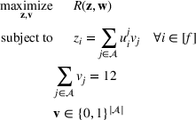
Jury selection formulation

In the jury selection problem, the lawyer has to select a subset
$S$
of jurors from a larger pool of available jurors
$A$
. In most jurisdictions, the number of jurors chosen is 12 (
$| S | = 12$
). In all generality, the probability a jury will return a guilty verdict is a function of the set of jurors chosen, and the inherent biases they might possess. Suppose each juror j has a vector of features
$u^{j}$
(education, religion, etc—see Table 6) which are relevant in predicting their likelihood of voting guilty. We assume the probability of a jury returning a guilty verdict can be modeled using a function
$R (z, w)$
where
$z$
are aggregate jury features, which are additive in the features of the jurors it comprises of
$z = \sum_{j \in S} u^{j}$
; for example, the number of jurors with post‐graduate education is the sum of the jurors who have post‐graduate education. The vector
$w$
is case‐dependent data that the lawyer have no control over, but still may affect the outcome of the case. An example of this is the gender of the victim, which the data suggest interacts with the gender of the juror to influence the verdict. We will restrict our attention to when
$R (z, w)$
is a random forest.

Two main objectives could be considered when choosing a jury: (i) choosing the fairest jury or (ii) choosing a jury that is most likely to return an outcome desired by the lawyer. Both objectives can be modeled under our framework. To align with the lawyer's goals, we would either maximize the probability of returning a guilty verdict by setting the objective to be
$\max_{z} R (z, w)$
as a prosecuting lawyer, or minimize the probability of returning the guilty score as a defending lawyer. To align with the state's goal of selecting the most fair jury, we could set the objective to be
$\min_{z} | R (z, w) - \bar{R} (w)) |$
, where
$\bar{R} (w)$
is the probability of a jury selected from the population at random returning a guilty verdict for a trial with features
$w$
. We define
$v_{j}$
as a binary variable, with
$v_{j} = 1$
if we choose to include juror j in the jury, 0 otherwise, and let f be the number of features of the jury we have data on. We can formulate the jury selection problem for the prosecuting lawyer as follows:
$\begin{matrix} \underset{z, v}{maximize} & R (z, w) \\ subject to & z_{i} = \sum_{j \in A} u_{i}^{j} v_{j} \forall i \in [f] \\ \sum_{j \in A} v_{j} = 12 \\ v \in {0, 1}^{| A |} \end{matrix}$
31

Simulations for optimizing a given forest

In this section, we explore the performance of the various random forest optimization procedures we have proposed in Sections 3.2 and 4. Note that this section is a comparison of how well the algorithms do in optimizing over given a random forest, rather than an analysis of how good random forest optimization is at selecting solutions, which we explore in Section 5.4.1. First, in Section 5.3.2, we test the speed of Benders decomposition compared to the standard MIP formulation, then in Section 5.3.3, we test the accuracy and speed of the cross‐validation performance compared to the MIP. We test the sensitivity of the algorithms discussed with the key parameter of our model; the number of trees in the random forest. Finally, in Section 5.3.4, we provide simulations that compare our approach of optimizing over a subset of trees of full depth to an alternative heuristic suggested in Mišić (2020), which instead truncates the depth of trees in the forest and optimizes over a shallower forest.

Testing environment

The random forests are trained on the datasets in Python using Scikit‐learn RandomForestRegressor and RandomForestRegression from Pedregosa et al. (2011) for jury and property selection, respectively. The optimization formulations were coded in Python and solved using a Gurobi 6.5 solver. For the jury selection problem, the juror pool size used was 20, while in the property investment problem, the number of vacant lots to choose between was 10.

Benders decomposition comparison

The solution times of the different algorithms are shown in Figure 4. As expected, the MIP formulation displays exponential behavior with respect to the number of trees in the random forest. It is very fast for small to medium‐sized problem instances up to 160 trees on the jury dataset (9100 nodes) and 80 trees on the housing dataset (35840 nodes) but takes prohibitively long for forests larger than this. For random forest instances larger than 500 trees on the jury dataset and 300 trees on the housing dataset, the MIP did not solve within the imposed solve limit of 1000 s. The MIP formulation with Benders cuts is slower than the MIP formulation for a small number of trees, but for forests larger than 200 trees on the jury dataset and 100 trees on the housing dataset, Benders is faster. The initial lag of the Benders formulation might be due to Gurobi's effective presolve techniques which are unable to be applied to the MIP formulation with Benders cuts because the master problem starts with very few constraints. As the problem grows larger, the benefits of Benders cuts outweigh the presolve.

FIGURE 4
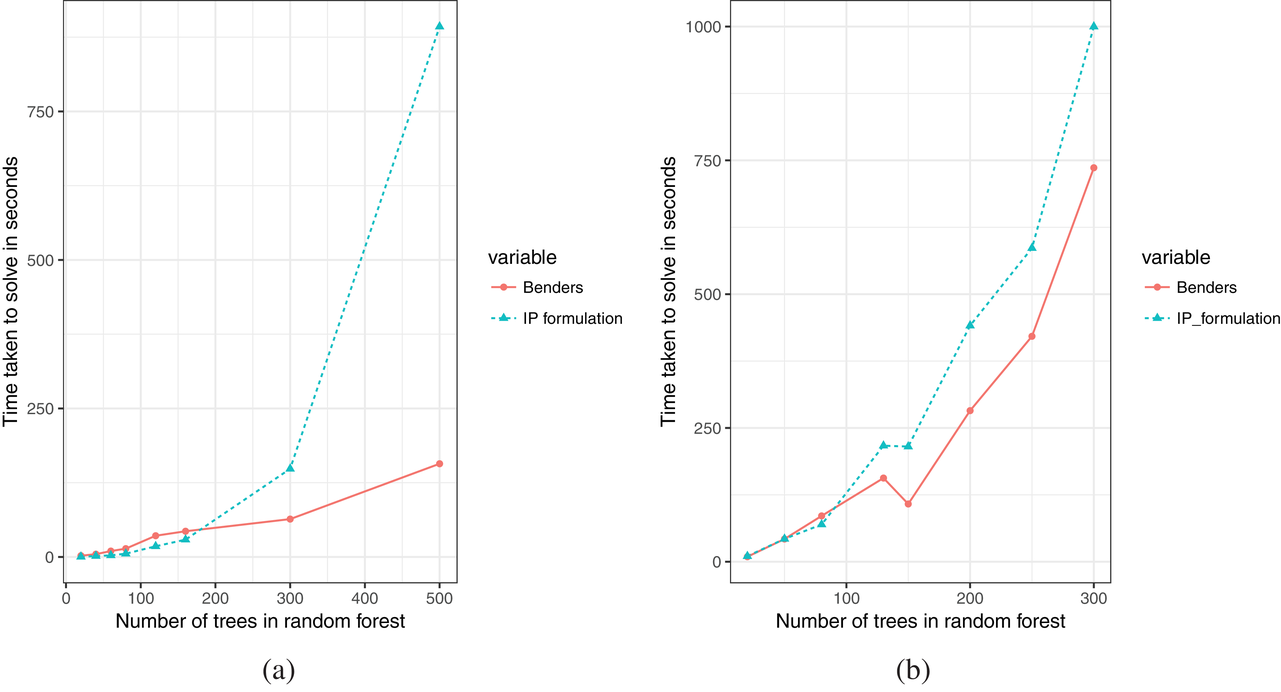
Time taken to solve algorithms for increasing forest size. (a) On the jury dataset. (b) On the housing dataset

Cross‐validation experiments

For each of these experiments, there is a target forest to optimize over, with the number of nodes in that forest given by
$N_{n o d e s}$
(this is an indication of the size of each tree). We compare solving the MIP for this target forest, versus splitting the forest into a number of subsets, solving each one using the MIP, and using cross‐validation to find the best solution.

Tables 8 and 9 show the performance of the cross‐validation algorithms relative to the MIP formulation, both in terms of the percentage of time taken to solve and the score of the cross‐validation solution as a percentage of the optimal MIP solution for the jury and housing datasets. We observe that the cross‐validation procedure can achieve a large percentage of optimality in a fraction of the time taken to solve the full MIP. This is surprising since the forests that cross‐validation is optimizing over are just one‐tenth or twentieth of the size of the target forest for the jury and housing datasets, respectively. Cross‐validation is particularly effective for the jury dataset, where the solve times are less than 10% of the MIP, but achieve over 95% of the accuracy if parameters are chosen correctly. This is because there is high variance in the predictions associated with the jury dataset (each forest subset has comparatively low accuracy), so there is significant value in validating the score of the jury chosen using different forests to the one it was chosen with. This suggests more broadly that cross‐validation is more valuable on noisy datasets where it is difficult to train accurate models. We note the % optimality is not guaranteed to be monotone because the subsets chosen for each experiment are independent. We further explore the behavior of cross‐validation with additional numerical experiments in Section S3.

TABLE 8
Cross‐validation performance on the jury dataset

# trees target 80 $(N_{n o d e s} = 4537)$ 300
$(N_{n o d e s} = 16238)$

# subsets 20 10 5 2 20 10 5 2

# trees per subset 4 4 4 4 15 15 15 15

% optimality 96.25% 96.25% 91.25% 66.25% 98.67% 98.67% 96.67% 81.67%

% time taken 5.55% 3.12% 1.74% 0.92% 12.51% 7.18% 5.12% 3.32%

TABLE 9
Cross‐validation performance on the housing dataset

# trees target 40 $(N_{n o d e s} = 66848)$ 60
$(N_{n o d e s} = 96792)$

# subsets 10 5 2 1 10 5 2 1

# trees per subset 4 4 4 4 6 6 6 6

% optimality 98.5% 96.9% 83.6% 92.8% 100.0% 99.1% 93.9% 93.9%

% time taken 89.0% 45.1% 17.4% 8.7% 74.0% 35.4% 13.6% 6.7%

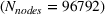
Comparison with depth restricted trees

We use the datasets wine, solubility, and concrete studied in Mišić (2020) and housing, which are described in Section 4.2. We train a large target random forest of 500 trees, with maximum depth 7 and default settings from Scikit‐learn RandomForestRegressor. For the depth‐restricted trees, we repeat trials where trees are truncated at a depth of 1–6 using all 500 trees. For the fewer trees approach, we optimize over a subset of
${5, 7, 11, 15, 20, 40, 60, 80, 120, 200}$
trees. We compare the time taken to find a solution using the MIP formulation to the solution quality as evaluated on the full random forest. We use a time limit of 300 s and only show the outcomes where a solution was found within this range.

The results are shown in Figure 5. We observe that for the solubility and concrete datasets, optimizing over a subset of trees is consistently faster and quicker than the tree methods with a truncated depth. For the other datasets, the results are comparable.

FIGURE 5
Time versus score for truncated tree depth and forest subset heuristics. (a) House dataset. (b) Solubility dataset. (c) Wine dataset. (d) Concrete dataset

In addition, changing the number of trees provides much more flexibility than truncating the depth of trees in achieving the quality versus time taken trade‐off. When truncating the depth of trees, the total number of nodes in the problem changes by approximately a factor of 2 every time the depth is increased by one layer. Since the MIP is exponential in solve time, this can be the difference between a problem that solves in seconds, compared to hours (if not days). It is not possible to collect any information about the quality of the solution between these points. In comparison, the change in the number of nodes we are optimizing over is linear in the number of trees, making this an easier tool in terms of experimentation.

Comparison with optimizing over other machine learning objective functions

In this section, we compare optimizing over a random forest objective function compared to optimizing over other simple, yet commonly used objective functions derived from linear or logistic regression.

Testing environment

In most real‐world datasets, we do not observe the counterfactual outcomes associated with different actions from those taken in the data. In particular, we cannot observe the actual outcome for the solutions we select with our optimization procedure, so we need a way to estimate the effectiveness of the random forest optimization methodology compared to other choices of machine learning objective functions.

We train multiple machine learning functions from the training data and choose the best solution as evaluated by each function. This is to compare the random forest solution with the solution that would be found if we optimized over a different machine learning function. For the jury selection (classification) problem, we compare the juries selected using a random forest, a linear regression and a logistic regression objective function, respectively,
$F_{R F}^{t r a i n} (x), F_{L i n}^{t r a i n} (x), F_{L o g}^{t r a i n} (x)$
to obtain
$x_{R F}^{}, x_{L i n}^{}, x_{L o g}^{}$
. For the property investment (regression) problem, we select vacant lots and build houses using a random forest and linear regression objective function
$F_{R F}^{t r a i n} (x), F_{L i n}^{t r a i n} (x)$
to obtain
$x_{R F}^{}, x_{L i n}^{}$
.

Next, we need to measure the performance of these solutions. We propose evaluating the performance of each solution using a range of different machine learning functions trained on an independent testing dataset. For the jury selection problem, we evaluate the juries chosen using a random forest evaluator
$F_{R F}^{t e s t} (x)$
and a logistic regression evaluator
$F_{L o g}^{t e s t} (x)$
. We choose the random forest as a test classifier because it has the highest predictive accuracy and choose the logistic regression test classifier to avoid any possible bias in using a random forest structure for training and testing. For the property investment problem, we evaluate the houses using a random forest and XGBoost objective function
$F_{R F}^{t e s t} (x), F_{X G B}^{t e s t} (x)$
due to the predictive accuracy of these models. To give us a reasonable sample size, we set
$K = 100$
(repeat this procedure 100 times for randomly sampled juror pools and different vacant lots). This process is summarized in Algorithm 2.

ALGORITHM 2
Out‐of‐sample testing procedure

1: Split the jury dataset into a training set and testing set.

2: Train different selection machine learning functions $F_{\mod}^{train} (x)$ from the training data, for all
$m o d \in {R F, L i n, L o g} = M$
.

3: Train different evaluation machine learning functions
$F_{\mod'}^{test} (x)$
from the test data for all
${m o d}^{'} \in M$
.

4: for k in
${1, …, K}$
do

5: Select an optimal solution for scenario
$w_{k}$
and each model,
$x_{\mod, k}^{} = \arg ma x_{x \in X_{k}} F_{\mod}^{train} (x)$

6: Evaluate each solution OOS with different all evaluators, for all
$m o d, {m o d}^{'} \in M F_{\mod'}^{test} (x_{\mod, k}^{})$

7: Take average over K trials.

Results for the jury selection case

Figure 6 shows the performance of juries chosen via various approaches.² For this simulation, we assume the optimizer is a prosecution lawyer who is trying to get a guilty verdict. Figure 6 shows the number of juries that were classified as guilty by the out‐of‐sample evaluators out of the 100 randomly drawn juror pools. We observe that optimization over the random forest objective outperforms optimization over the other objectives when evaluated using both the random forest and logistic regression evaluators. Of particular interest is that the random forest optimization outperforms the logistic regression even using the logistic regression evaluator. This may be due to the higher out‐of‐sample predictive accuracy of the random forest (60%) compared to either logistic regression (56%) or linear regression (49%). Interestingly, the improvement in the number of convictions using random forest (+10%) is greater than the improvement in predictive accuracy using a random forest (+4%).

FIGURE 6
Number of juries (out of 100) which are predicted to return a guilty verdict according to out‐of‐sample model, if optimized for guilty verdict. (a) Random forest evaluator
$F_{R F}^{t e s t} (\cdot)$
. (b) Logistic regression evaluator
$F_{L o g}^{t e s t} (\cdot)$

Results for the property investment case

Table 10 shows the sale price of property chosen using random forest minus the sales price of a property chosen by linear regression, as evaluated on an out‐of‐sample XGBoost
$F_{X G B}^{t e s t} (x_{R F}^{}) - F_{X G B}^{t e s t} (x_{l i n}^{})$
. Likewise Table 11 evaluates using an out‐of‐sample random forest
$F_{R F}^{t e s t} (x_{R F}^{}) - F_{R F}^{t e s t} (x_{l i n}^{*})$
. The results shown are averaged over 100 different sets of vacant lots being available and repeated for the property investor choosing from a set of 5, 10, or 20 vacant lots. We observe improvements when choosing properties using a random forest objective compared to a linear regression objective for each lot choice size and for both evaluators. The performance appears slightly better when evaluated on random forest compared to XGBoost. We observe the difference increases with the number of lots we consider, from around 3% with 5 lots to over 15% with 20 lots. This is because the random forest is particularly good at selecting valuable properties due to the nonlinear relationship between latitude, longitude, and price. We believe these experiments show the clear advantages to optimizing using a random forest objective function compared to other machine learning functions.

TABLE 10
Difference in sale price of the property chosen using random forest (RF) versus linear regression as evaluated on OOS XGBoost

Number of lots to choose between 10 lots 20 lots 40 lots

Average improvement using RF 9.08 % 16.9 % 20.1 %

p value for significance of difference $1.5 \times 10^{- 6}$
$8.0 \times 10^{- 13}$

$6.4 \times 10^{- 15}$

TABLE 11
Difference in sale price of property chosen using random forest (RF) versus linear regression as evaluated on OOS random forest

Number of lots to choose between 10 lots 20 lots 40 lots

Average improvement using RF 11.4 % 19.2 % 25.6 %

p value for significance of difference $1.5 \times 10^{- 7}$
$3.1 \times 10^{- 14}$

$1.1 \times 10^{- 15}$

Synthetic data

To overcome the issue of not being able to observe the counterfactuals in real datasets, we also ran experiments on synthetic data. With these datasets, it is possible to evaluate exactly how well each option does since we know what the counterfactuals are. We used the synthetic datasets from Friedman et al. (1991), which is a well‐known benchmark dataset in the machine learning community. The datasets tested are:
Friedman 1:
$y (X) = 10 \sin (π X_{0} \cdot X_{1}) + 20 {(X_{2} - 0.5)}^{2} + 10 X_{3} + 5 X_{4} + N (0, 1)$
with
$X_{i} \sim U (0, 1), i \in {1, … 10}$
, where
$X_{5}, . ., X_{10}$
are additional noise.

Friedman 2:
$y (X) = {(X_{0}^{2} + {(X_{1} \cdot X_{2} - 1 / (X_{1} \cdot X_{3}))}^{2})}^{0.5} + N (0, 1)$
, with
$X_{0} \sim U (0, 100), X_{1} \sim U (40 π, 560 π), X_{2} \sim U (0, 1), X_{3} \sim U (1, 11)$
.

We compare learning and optimizing over a linear function, a CART tree, and a random forest with 10 trees. 2000 data points are used for training the models. In both cases, we solve
$\min_{x} y (x)$
, subject to the constraint that
$x$
must be in the domain of the data (i.e
$0 \leq X_{0} \leq 100$
for the Friedman 2 dataset). We then find the optimal solution
$x_{o p t}^{i}$
for sample, and calculate the true outcome
$y (x_{o p t}^{i})$
. We repeat this process 100 times to get a distribution over
$y (x_{o p t}^{i})$
, which is shown in Figure 7. The confidence bars are at 10% and 90% respectively. As can be seen in Figure 7, the random forest typically performs better than the CART, which in turn is better than the linear regression. There also appears to be less variance in the solution of the random forest relative to the CART model. The linear regression has no variance, achieving the same solution every time, although that solution is often poor. An issue with using a linear objective function is that the solution will always be at the edge of the feasible set, even when the optimal solution is at the interior.

FIGURE 7
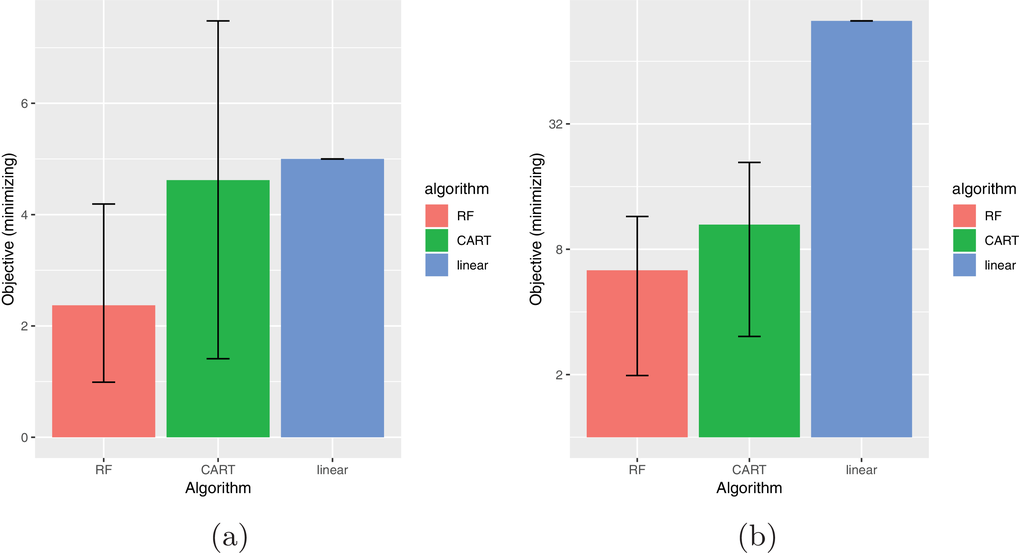
Performance on synthetic data. (a) Friedman 1 dataset. (b) Friedman 2 dataset

CONCLUSIONS

In this paper, we examine a data‐driven optimization approach, where an uncertain objective is estimated according to a machine learning function. In particular, we have shown that it is possible to optimize over a random forest objective function with general polyhedral constraints using mixed‐integer linear programming. Including constraints in our approach allows us to model many problems of practical interest as well as to define a policy class for our decisions, which can be useful for interpretable decision‐making. While the efficacy of this approach depends on the predictive accuracy of random forest relative to other predictive models, and the time available to find a solution, this approach has many advantages. First, random forests are a very powerful prediction algorithm that can fit unknown nonlinear and complex interactions of features with minimal feature engineering. Second, random forests often perform very well in practice, with high prediction accuracy. Third, we can leverage existing MIP solvers which are effective at solving large‐scale complex problems and provide flexibility to model a wide range of problems. We demonstrate the effectiveness of this approach at solving real‐world problems using a case study on jury selection and property investment and show this method outperforms other machine learning objective functions. We also show that it is possible to achieve significant speed improvements using Benders cuts for large‐scale problems.

For large‐scale random forests, we propose an algorithm for approximating a random forest with a limited number of trees and show analytical bounds on the probability of being suboptimal by a given amount. In particular, for trees with axis‐aligned splits, we show that the number of trees we need to sample to be within ε of the optimal solution with a probability
$1 - δ$
is sublinear in the size of the forest being approximated. These insights lead us to develop a heuristic approach inspired by cross‐validation applied to an optimization setting. We show that these heuristics perform well on the jury and housing data, getting solutions close to the MIPs in a fraction of time. Furthermore, we show that in some datasets, this results in significant improvement over existing heuristics that optimize over trees of truncated depth.

Footnotes
1
When dealing with a degenerate subproblem with multiple optimal dual solutions, the Magnanti and Wong () method selects the solution that is the closest to the interior of the master problem polyhedron.
2
We fixed the case features for each of the trials we selected a jury for and selected a juror pool by bootstrapping from the juror population. Note that the results below are for a difficult instance of the problem; the case type makes a conviction unlikely, so the appropriate benchmark is the likelihood of conviction for a randomly selected jury, not 50%.
ORCID iD
Max Biggs
Georgia Perakis
References
1.
Aggarwal C. C. Chen C. Han J. (2010). The inverse classification problem. Journal of Computer Science and Technology, 25(3), 458–468.
2.
Amram M. Dunn J. Zhuo Y. D. (2022). Optimal policy trees. Machine Learning, 111(7), 2741–2768.
3.
Anderson R. Huchette J. Ma W. Tjandraatmadja C. Vielma J. P. (2020). Strong mixed‐integer programming formulations for trained neural networks. Mathematical Programming, 183(1), 3–39.
4.
Aouad A. Elmachtoub A. N. Ferreira K. J. McNellis R. (2019). Model trees for personalization. arXiv preprint arXiv:1906.01174.
5.
Athey S. Imbens G. (2016). Recursive partitioning for heterogeneous causal effects. Proceedings of the National Academy of Sciences, 113(27), 7353–7360.
6.
Athey S. Tibshirani J. Wager S. (2019). Generalized random forests. The Annals of Statistics, 47(2), 1148–1178.
7.
Baardman L. Cohen M. C. Panchamgam K. Perakis G. Segev D. (2019). Scheduling promotion vehicles to boost profits. Management Science, 65(1), 50–70.
8.
Ban G.‐Y. El Karoui N. Lim A. E. (2016). Machine learning and portfolio optimization. Management Science .
9.
Ban G.‐Y. Keskin N. B. (2021). Personalized dynamic pricing with machine learning: High‐dimensional features and heterogeneous elasticity. Management Science, 67(9), 5549–5568.
10.
Ban G.‐Y. Rudin C. (2018). The big data newsvendor: Practical insights from machine learning. Operations Research, 67(1), 90–108.
11.
Barbella D. Benzaid S. Christensen J. M. Jackson B. Qin X. V. Musicant D. R. (2009). Understanding support vector machine classifications via a recommender system‐like approach. DMIN , Las Vegas, NV.
12.
Bertsimas D. Dunn J. (2017). Optimal classification trees. Machine Learning, 106(7), 1039–1082.
13.
Bertsimas D. Kallus N. (2020). From predictive to prescriptive analytics. Management Science, 66(3), 1025–1044.
14.
Bertsimas D. OHair A. Relyea S. Silberholz J. (2016). An analytics approach to designing combination chemotherapy regimens for cancer. Management Science, 62(5), 1511–1531.
15.
Besbes O. Phillips R. Zeevi A. (2010). Testing the validity of a demand model: An operations perspective. Manufacturing & Service Operations Management, 12(1), 162–183.
16.
Biau G. Scornet E. (2016). A random forest guided tour. Test, 25(2), 197–227.
17.
Biggs M. Perakis G. (2019). Dynamic routing with tree based value function approximations [Ph.D. thesis, Massachusetts Institute of Technology].
18.
Biggs M. Sun W. Ettl M. (2021). Model distillation for revenue optimization: Interpretable personalized pricing. In Proceedings of the 38th International Conference on Machine Learning , (pp. 946–956). PMLR.
19.
Breiman L. (1996). Bagging predictors. Machine Learning, 24(2), 123–140.
20.
Breiman L. (2001). Random forests. Machine Learning, 45(1), 5–32.
21.
Chen T. Guestrin C. (2016). Xgboost: A scalable tree boosting system. In Proceedings of the 22Nd ACM SIGKDD International Conference on Knowledge Discovery and Data Mining , (pp. 785–794). ACM.
22.
Chen X. Owen Z. Pixton C. Simchi‐Levi D. (2022). A statistical learning approach to personalization in revenue management. Management Science, 68(3), 1591–2376.
23.
Chi C.‐L. Street W. N. Robinson J. G. Crawford M. A. (2012). Individualized patient‐centered lifestyle recommendations: An expert system for communicating patient specific cardiovascular risk information and prioritizing lifestyle options. Journal of Biomedical Informatics, 45(6), 1164–1174.
24.
Cohen M. C. Lobel I. Paes Leme R. (2020). Feature‐based dynamic pricing. Management Science, 66(11), 4921–4943.
25.
Cortez P. Cerdeira A. Almeida F. Matos T. Reis J. (2009). Modeling wine preferences by data mining from physicochemical properties. Decision Support Systems, 47(4), 547–553.
26.
Denove C. F. Imwinkelried E. J. (1995). Jury selection: An empirical investigation of demographic bias. American Journal of Trial Advocacy, 19, 285.
27.
Elmachtoub A. N. Grigas P. (2022). Smart “predict, then optimize”. Management Science, 68(1), 9–26.
28.
Ferreira K. J. Lee B. H. A. Simchi‐Levi D. (2015). Analytics for an online retailer: Demand forecasting and price optimization. Manufacturing & Service Operations Management, 18(1), 69–88.
29.
Fischetti M. Jo J. (2018). Deep neural networks and mixed integer linear optimization. Constraints, 23(3), 296–309.
30.
Freund Y. Schapire R. E. (1997). A decision‐theoretic generalization of on‐line learning and an application to boosting. Journal of Computer and System Sciences, 55(1), 119–139.
31.
Friedman J. H. (1991). Multivariate adaptive regression splines. The Annals of Statistics, 19(1), 1–67.
32.
Hannaford‐Agor P. L. Hans V. P. Mott N. L. Munsterman G. T. (2003). Evaluation of hung juries in bronx county, new york, los angeles county, california, maricopa county, arizona, and washington, dc, 2000–2001. National Center for State Courts User Guide. National Center for State Courts .
33.
Harlfoxem (2016). House sales in king county, usa. https://www.kaggle.com/harlfoxem/housesalesprediction
34.
Hartje R. (2004). A jury of your peers: How jury consulting may actually help trial lawyers resolve constitutional limitations imposed on the selection of juries. California Western Law Review, 41, 479.
35.
Huuskonen J. (2000). Estimation of aqueous solubility for a diverse set of organic compounds based on molecular topology. Journal of Chemical Information and Computer Sciences, 40(3), 773–777.
36.
Kallus N. (2017). Recursive partitioning for personalization using observational data. In International Conference on Machine Learning , (pp. 1789–1798). PMLR.
37.
Ke G. Meng Q. Finley T. Wang T. Chen W. Ma W. Ye Q. Liu T.‐Y. (2017). Lightgbm: A highly efficient gradient boosting decision tree. Advances in Neural Information Processing Systems, 30, 3146–3154.
38.
Kleywegt A. J. Shapiro A. Homem‐de Mello T. (2002). The sample average approximation method for stochastic discrete optimization. SIAM J. on Optimization, 12(2), 479–502. https://doi.org/10.1137/S1052623499363220
39.
Lash M. T. Zhao K. (2016). Early predictions of movie success: The who, what, and when of profitability. Journal of Management Information Systems, 33(3), 874–903.
40.
Magnanti T. L. Wong R. T. (1981). Accelerating benders decomposition: Algorithmic enhancement and model selection criteria. Operations Research, 29(3), 464–484.
41.
Mercier A. Cordeau J.‐F. Soumis F. (2005). A computational study of benders decomposition for the integrated aircraft routing and crew scheduling problem. Computers & Operations Research, 32(6), 1451–1476. https://doi.org/10.1016/j.cor.2003.11.013. http://www.sciencedirect.com/science/article/pii/S0305054803003447
42.
Mišić V. V. (2020). Optimization of tree ensembles. Operations Research, 68(5), 1605–1624.
43.
Moselle B. (2015). National building cost manual. Craftsman Book Company .
44.
Pedregosa F. Varoquaux G. Gramfort A. Michel V. Thirion B. Grisel O. Blondel M. Prettenhofer P. Weiss R. Dubourg V. Vanderplas J. Passos A. Cournapeau D. Brucher M. Perrot M. Duchesnay E. (2011). Scikit‐learn: Machine learning in python. Journal of Machine Learning Research, 12(Oct), 2825–2830.
45.
Pendharkar P. C. (2002). A potential use of data envelopment analysis for the inverse classification problem. Omega, 30(3), 243–248.
46.
Qian M. Murphy S. A. (2011). Performance guarantees for individualized treatment rules. Annals of statistics, 39(2), 1180.
47.
Rockafellar R. T. (1970). Convex analysis. Vol. 18, Princeton University Press.
48.
Santoso T. Ahmed S. Goetschalckx M. Shapiro A. (2005). A stochastic programming approach for supply chain network design under uncertainty. European Journal of Operational Research, 167(1), 96–115. http://EconPapers.repec.org/RePEc:eee:ejores:v:167:y:2005:i:1:p:96‐115
49.
Steele J. M. (2004). The Cauchy‐Schwarz master class: An introduction to the art of mathematical inequalities. Cambridge University Press.
50.
Tang L. Jiang W. Saharidis G. K. (2013). An improved benders decomposition algorithm for the logistics facility location problem with capacity expansions. Annals of Operations Research, 210(1), 165–190.
51.
Tjeng V. Xiao K. Tedrake R. (2017). Evaluating robustness of neural networks with mixed integer programming. arXiv preprint arXiv:1711.07356.
52.
Wager S. Athey S. (2018). Estimation and inference of heterogeneous treatment effects using random forests. Journal of the American Statistical Association, 113(523), 1228–1242.
53.
Yang C. Street N. W. Robinson J. G. (2012). 10‐year cvd risk prediction and minimization via inverse classification. In Proceedings of the 2nd ACM SIGHIT International Health Informatics Symposium (pp. 603–610). ACM.
54.
Yeh I.‐C. (1998). Modeling of strength of high‐performance concrete using artificial neural networks. Cement and Concrete research, 28(12), 1797–1808.
Supplementary Material
Please find the following supplemental material available below.
For Open Access articles published under a Creative Commons License, all supplemental material carries the same license as the article it is associated with.
For non-Open Access articles published, all supplemental material carries a non-exclusive license, and permission requests for re-use of supplemental material or any part of supplemental material shall be sent directly to the copyright owner as specified in the copyright notice associated with the article.
0.00 MB
0.48 MB

		Dimension
Dataset	Model	1	2	3	4	5
house	Linear	0.55	0.83	0.98	0.99	0.99
	Exponential	0.55	0.73	0.69	0.58	0.55
	Multiplicative	0.93	0.99	0.98	0.99	0.91
solubility	Linear	0.67	0.74	0.53	0.72	0.72
	Exponential	0.59	0.60	0.51	0.61	0.58
	Multiplicative	0.91	0.88	0.90	0.94	0.90
wine	Linear	−0.40	0.99	0.99	1.00	1.00
	Exponential	−0.15	0.62	0.65	0.76	0.77
	Multiplicative	0.73	0.93	0.98	1.00	1.00
concrete	Linear	0.58	1.00	0.99	0.99	0.99
	Exponential	0.55	0.53	0.41	0.40	0.36
	Multiplicative	0.90	0.85	0.79	0.79	0.72

	Dimension
Dataset	1	2	3	4	5
house	0.28	0.39	0.91	1.43	1.38
solubility	0.46	0.63	0.37	0.43	0.58
wine	0.14	1.19	1.30	0.92	0.91
concrete	0.39	1.53	1.93	1.98	2.07

1:	Train τ forests $R_{1} (\cdot), …, R_{τ} (\cdot)$ on the data
2:	Find optimal solution for each forest $x_{i} = {arg max}_{x \in X} R_{i} (x) \forall i \in [τ]$
3:	Calculate $\bar{R} (x_{i}) = \frac{1}{τ} \sum_{j} R_{j} (x_{i}) \forall i \in [τ]$
4:	Pick $x^{C V} = {arg max}_{i \in [τ]} \bar{R} (x_{i})$

House variables	Meaning	Lot variables	Meaning
bedrooms	Number of bedrooms	zipcode	Zipcode house is located in
bathrooms	Number of bathrooms	lat	Latitude of house
size	Square footage of the home	lon	Longitude of house
base	Square footage of the basement	sqftlot	Square footage of the lot
grade	Quality of construction	water	View of waterfront (binary)

Model	Training accuracy (R ²)	Testing accuracy (R ²)
Random forest	98	88
XGBoost	100	90
CART	99	76
Ridge regression	70	70
Linear regression (OLS)	70	69

Jury variables	Meaning	Case variables	Meaning
police	Trust the police	deftgend	Defendant's gender
amcourts	Trust the courts	defrace	Defendant's race
crmsevre	Think crime serious problem	victgend	Victim's gender
previous	Been a juror before	victrace	Victim's race
civilcrm	Previous jury‐criminal of civil	victrela	Victim's relationship to defendant
gender	Gender	casetype	Case type
age	Age
school	Highest level of education
race	Race/ethnicity
religion	Strength of religious beliefs
income	Household income
jobstat	Job status
occupat	Occupation

# trees target	80 $(N_{n o d e s} = 4537)$				300 $(N_{n o d e s} = 16238)$
# subsets	20	10	5	2	20	10	5	2
# trees per subset	4	4	4	4	15	15	15	15
% optimality	96.25%	96.25%	91.25%	66.25%	98.67%	98.67%	96.67%	81.67%
% time taken	5.55%	3.12%	1.74%	0.92%	12.51%	7.18%	5.12%	3.32%

1:	Split the jury dataset into a training set and testing set.
2:	Train different selection machine learning functions $F_{\mod}^{train} (x)$ from the training data, for all $m o d \in {R F, L i n, L o g} = M$ .
3:	Train different evaluation machine learning functions $F_{\mod'}^{test} (x)$ from the test data for all ${m o d}^{'} \in M$ .
4:	for k in ${1, …, K}$ do
5:	Select an optimal solution for scenario $w_{k}$ and each model, $x_{\mod, k}^{*} = \arg ma x_{x \in X_{k}} F_{\mod}^{train} (x)$
6:	Evaluate each solution OOS with different all evaluators, for all $m o d, {m o d}^{'} \in M F_{\mod'}^{test} (x_{\mod, k}^{*})$
7:	Take average over K trials.

Number of lots to choose between	10 lots	20 lots	40 lots
Average improvement using RF	9.08 %	16.9 %	20.1 %
p value for significance of difference	$1.5 \times 10^{- 6}$	$8.0 \times 10^{- 13}$	$6.4 \times 10^{- 15}$

Number of lots to choose between	10 lots	20 lots	40 lots
Average improvement using RF	11.4 %	19.2 %	25.6 %
p value for significance of difference	$1.5 \times 10^{- 7}$	$3.1 \times 10^{- 14}$	$1.1 \times 10^{- 15}$

Constrained optimization of objective functions determined from random forests

Abstract

Keywords

INTRODUCTION

Contributions

RELEVANT LITERATURE

Data‐driven optimization

Relation to causal inference

MODEL

MIP formulation

Benders decomposition

APPROXIMATING LARGE RANDOM FORESTS

Analytical results

Number of sets in a random forest: a simulation study

Cross‐validation for optimization

NUMERICAL EXPERIMENTS

Case study: Property investment

Prediction

Formulation

Jury selection case study

Background

Predicting jury verdict

Jury selection formulation

Simulations for optimizing a given forest

Testing environment

Benders decomposition comparison

Cross‐validation experiments

Comparison with depth restricted trees

Comparison with optimizing over other machine learning objective functions

Testing environment

Results for the jury selection case

Results for the property investment case

Synthetic data

CONCLUSIONS

Footnotes

1

2

ORCID iD

References

Supplementary Material