Sage Journals: Discover world-class research

Abstract

Building an electrocardiogram (ECG) heartbeat classification model is essential for early arrhythmia detection. This research aims to build a reliable model that can classify heartbeats into five heartbeat types: normal beat (N), supraventricular ectopic beat (SVEB), ventricular ectopic beat (VEB), fusion beat (F), and unknown beat (Q), with a focus on enhancing the predictions of the uncommon Q and F heartbeats. The base dataset used is the MIT-BIH SupraVentricular Database, which was used to train and compare the performance of five machine learning models: logistic regression, Random Forest (RF), K-nearest neighbor, linear support vector machine, and linear discriminant analysis. In addition to using the synthetic minority oversampling technique, data extracted from multiple databases for the F and Q classes were combined with the original base dataset. These methods resulted in significant improvement in the recall for the rare F and Q classes when compared to the literature. The RF algorithm produced the best performance with an accuracy of 97% and recall values equal to 97%, 93%, 95%, 95%, and 30% for N, SVEB, VEB, F, and Q, respectively.

Keywords

ECG classification machine learning fusion beat unknown beat random forest

Introduction

According to data from the World Health Organization (WHO), the leading causes of death globally in the past few years have been cardiovascular diseases, including coronary artery disease, stroke, and heart failure.¹ Arrhythmia, or abnormal heart rhythms, can be a symptom of cardiovascular disease or a risk factor for developing one. For example, arrhythmia can result from damage to the heart muscle due to a heart attack or other forms of heart damage.

According to Mayo Clinic, arrhythmia can be defined as irregular heartbeats when the electrical signals that coordinate the heart's beats do not function properly.^2,3 Early arrhythmia detection is essential because it can help to identify and treat abnormal heart rhythms at an early stage, which can help to prevent or manage serious complications. When arrhythmia is not detected and treated early, it can cause various symptoms, including palpitations, dizziness, shortness of breath, and fainting. It can also increase the risk of stroke and other serious complications. For example, myocardial infarction (MI), also known as a heart attack, is a silent and fatal cardiovascular disease that can cause sudden death without warning. Thus an accurate and automated ECG classification is critical in the diagnosis and treatment of heart diseases, as reported by Rai and Chatterjee⁴ in addition to being effective in the detection of cardiac arrhythmias, as they also reported in Rai and Chatterjee.^5,6

Several methods can be used to classify heartbeats, including manual analysis of electrocardiogram (ECG) tracings by trained healthcare providers or automated analysis employing machine learning algorithms. Both methods identify heartbeat features, such as the shape and duration of the various waves and complexes present in ECG tracing. Then, use these features to classify heartbeats into different categories as defined by the Association for the Advancement of Medical Instrumentation EC57 standard,⁷ shown in Table 1. Classifiers aim to build reliable models that can classify heartbeats into the five heartbeat super-classes: normal beat (N), supraventricular ectopic beat (SVEB), ventricular ectopic beat (VEB), fusion beat (F), and unknown beat (Q).

Table 1.

Heartbeat categories according to AAMI.

Heartbeat superclass	Heartbeat annotation
N (Normal)	N (Normal) L (Left bundle branch block beat) R (Right bundle branch block beat) e (Atrial escape beat) j (Nodal (junctional) escape beat)
SVEB (Supraventricular ectopic beat)	A (Atrial premature beat) a (Aberrated atrial premature beat) J (Nodal (junctional) premature beat) S (Supraventricular premature beat)
VEB (Ventricular ectopic beat)	V (Premature ventricular contraction) E (Ventricular escape beat)
F (Fusion beat)	F (Fusion of ventricular and normal beats)
Q (Unknown beat)	Q (Unclassifiable beat)/(Paced beat) f (Fusion of paced and normal beat)

Figure 1 shows a diagram of a typical ECG signal. The signal consists of three major parts: The P wave, the QRS complex, and the T wave. The diagram shows critical parameters like the PQ, ST, QRS, and QT intervals. These parameters constitute a key part of the features that will be used later in constructing the ECG classification model.

Figure 1.

ECG diagram.

While numerous studies in ECG classification have used machine learning techniques, most of them targeted achieving higher overall accuracy. Something that can be easily biased if you have an unbalanced distribution of classes. Overall accuracy can be easily manipulated by increasing the number of samples of an easy-to-detect class. This is the case for ECG datasets, as most contain a large percentage of the normal (N) class, which has a very high recall rate. In such cases, considering the per-class recall numbers would be a more accurate measure of the classifier's performance than the overall accuracy. The fact that the F and Q classes had the fewest instances in these datasets contributed to the poor performance of classification models in correctly identifying these classes. When a class has very few instances, it is more difficult for the model to learn its distinctive features and patterns. As a result, the model may not be able to generalize well and may struggle to classify new instances of that class correctly.

This work adds value to the existing literature on ECG classification using machine learning by explicitly focusing on improving the recall of the Q and F classes, which are often associated with severe cardiac conditions and often have the fewest number of instances in the datasets. This is a significant contribution, as many previous studies did not address the issue of the performance of these specific classes. Tackling the problem of uncommon heartbeats is done using two approaches. The first is deploying the synthetic minority oversampling technique (SMOTE), which oversamples the minority classes to create additional synthetic data. While the second relies on combining data for the minority classes from multiple datasets. Using these approaches together has shown tremendous improvement in the recall of the Q and F heartbeats. It is worth noting that the base dataset used in this work is the MIT-BIH Supraventricular Arrhythmia Database created by Greenwald.⁸

The remaining parts of the paper are organized as follows: the Related Work section presents the related literature regarding ECG heartbeat classification. The Dataset and Experimental Setup section will detail the primary datasets used and the experimental setup. The Machine Learning Algorithms section describes the machine algorithms used in this article. Meanwhile, the Results and Analysis section presents the results of the three cases: the original dataset, after using SMOTE, and when combining multiple datasets. Finally, the conclusion presents a summary of findings and future research direction.

Related work

Machine learning has been proven to be helpful in the medicinal field. For example, in the prediction of multiple diseases like diabetes,⁹ heart disease,^10,11 and strokes.¹² As for ECG heartbeat classification, several approaches have been taken regarding signal preprocessing and various models and implementations. Wang et al.¹³ have used the Easy Ensemble technique and global heartbeat information for an imbalanced heartbeat classification on the MIT-BIH arrhythmia dataset.¹⁴ The MIT-BIH arrhythmia dataset is similar to the MIT-BIH supraventricular arrhythmia dataset used in this research as it comes from the same holster records and thus has the same features but fewer instances. Wang et al. tested their database using the interpatient scheme. Their experimental results showed that the global heartbeat information is helpful for heartbeat classification and achieved an average accuracy of 95.6% and a recall of 91.7%, 89.9%, 87.8%, and 55.4% for types N, SVEB, VEB, and F, respectively.

Zhang et al.¹⁵ proposed a method that selects effective feature subsets for distinguishing a class from classes by performing a One-versus-One comparison on a support vector machine (SVM) binary classifier on the MIT-BIH Arrhythmia Database.¹⁴ Zhang et al. achieved recall values of 88.94%, 79.06%, 85.48%, and 93.81% for classes N, SVEB, VEB, and F.

Meanwhile, Diker used a different dataset and compared the results of three different models that used artificial neural networks, SVM, and k-nearest neighbor (KNN) and used a 10-fold crossvalidation method for better performance.¹⁶ They achieved the best results with the SVM model, achieving an accuracy of 85.1%.

Alarsan and Younes¹⁷ combined the MIT-BIH Supraventricular Arrhythmia Database⁸ and the MIT-BIH Arrhythmia Database¹⁴ to get a total of 205,146 instances. In addition, it was implemented using three models, Decision Trees, Random Forest (RF), and Gradient-Boosted Trees, and achieved the highest accuracy of 98.03% with RF for multiclassification.

Bhattacharyya et al.¹⁸ studied the effect of extracting 61 features using the time-series feature extraction library (TSFEL) and then applying a weighted majority ensemble of RF and SVM on the MIT-BIH arrhythmia dataset. The purpose of incorporating the TSFEL during feature extraction and the SMOTE is to create a more balanced dataset. The paper achieved an accuracy of 98.21% and recall values of 99.5%, 74.2%, 94.22%, 73.21%, and 0% for N, SVEB, VEB, F, and Q classes, respectively.

In addition, L. Wang¹⁹ proposed a new approach for arrhythmia classification using a three-heartbeat multi-lead (THML) ECG data, in which each fragment contained three complete heartbeat processes of multiple ECG leads. The THML ECG data preprocessing method is formulated, and four arrhythmia classification models are constructed using 1D-CNN and a priority model with an integrated voting method. The classification of the dual ECG lead with THML data achieved a recall of 96.37%, 96.99%, 80.47%, 22.75%, and 8.33% for N, VEB, SVEB, F, and Q classes. Table 2 shows a summary of the four key research papers, showing the pros and cons of each one of them.

Table 2.

Summary of the main related literature.

Literature	Pros	Cons
Z. Zhang et al. (2014)	Proposed automatic heartbeat classification using a disease-specific feature selection approach. Two independent training procedures are executed for the data acquired from each lead for evaluation.	Training data was not balanced. Class Q was discarded.
S. Bhattacharyya et al. (2021)	Implemented an Ensemble of RF and SVM using a weighted majority algorithm (WMA). Performed 10-fold crossvalidation on the training set.	Although high accuracy was achieved, the recall for the minority classes was relatively low, mapping to 74.2%, 73.21%, and 0% for SVEB, F, and Q, respectively.
T. Wang et al. (2022)	Adopt multiple features from the heartbeat (three types of local and global features). Used Easy Ensemble balancing technique and compared against other balancing methods like SMOTE.	The adopted features have different distributions, and direct concatenation may affect classification performance. Class Q was discarded.
L. Wang et al. (2022)	Proposed a novel method that uses a three-heartbeat multi-lead (THML). The majority voting method was used on four models.	The THML ECG data relies on the accuracy of the QRS wave detection algorithm.

Dataset and experimental setup

The work presented in this article creates a heartbeat classification model and studies the impact of adding multiple datasets on enhancing its performance in predicting the Q and F classes. The primary dataset used is the MIT-BIH supra-ventricular dataset,⁸ which will be referred to as the base dataset throughout the text. The other supplementary datasets used are:

The MIT-BIH arrhythmia dataset.¹⁴

The IN-CART 12-lead Arrhythmia Database.²⁰

The Sudden Cardiac Death Holter Database.²¹

All these datasets are available in the public domain and share similar features. Thus, data from these datasets can be merged simply by appending their records. The data merge process is focused on adding the Q and F classes to the primary dataset, whereas other instances are dropped.

Datasets

The MIT-BIH supraventricular dataset is a dataset that consists of 78 ECG recordings, each lasting about 30 minutes. The recordings were obtained from patients with various clinical conditions, including healthy individuals and those with structural heart disease, and were collected using the standard 12-lead ECG equipment. A 12-lead ECG is named as such because it records the heart's electrical activity from 12 different viewpoints or leads. The test uses ten electrodes, one attached to each of the four limbs and six to the chest. The four attached to the limbs create six views of the heart in the vertical plane (I, II, III, VL, VF, and VR). Meanwhile, the remaining six electrodes are attached to the chest and are responsible for the six views V1 to V6 that record the activity in the horizontal plane. Thus, the 12-lead ECG as a diagnostic test provides a complete picture of the heart's electrical activity, recording information from six limb leads and six chest leads.²² In the referenced dataset, only leads II and V5 were used.

The dataset consists of 184,428 instances, where each instance is a single ECG signal representing a single heartbeat. The dataset consists of 34 features, including one for the patient record and another for the heartbeat classification type (Label). The remaining 32 features are divided into 16 features representing the signals of lead II and 16 features representing the features of lead V5. The features of both leads are identical. The only difference is the placement of the electrodes on the body. Table 3 describes the features list.

Table 3.

Feature description.

Attribute	Description	Feature type
Record	A number assigned to the patient	Numeric
Type	Classification of heartbeat	Object
pre-RR	The period between the end of one R-R interval and the beginning of the next.	Numeric
post-RR	The period following the R-R interval.	Numeric
pPeak	The peak of the P wave.	Numeric
tPeak	The peak of the T wave.	Numeric
rPeak	The peak of the R wave.	Numeric
sPeak	The peak of the S wave.	Numeric
qPeak	Small, positive deflection in the QRS complex.	Numeric
qrs interval	Duration of the QRS complex.	Numeric
pq interval	The time between the P wave's start and the QRS complex's start.	Numeric
qt interval	The time between the start of the QRS complex, and the end of the T wave.	Numeric
st interval	The time between the S wave's end and the T wave's start.	Numeric
qrs morphologies	For the morphology features, five samples are taken in the QRS complex (between the on-set and off-set points of the QRS complex²³)	Numeric

Data attribute information

Figure 2 reveals the distribution of values for some features provided within the dataset. Figure 2(a) shows the sPeak distribution, where it can be seen that the number of instances grows increasingly from −4 mv toward zero, followed by a sharp drop in the number of instances toward the positive values. This indicates the normal range of “sPeak” varies within negative millivolts. Moreover, all intervallic features measured by millisecond are distributed between positive 1 ms up to 150 ms. For example, Figure 2(b) refers to qt-interval, where most instances are centered around 13 ms, while the pq-interval, shown in Figure 2(c), has the most instances at 2 ms.

Figure 2.

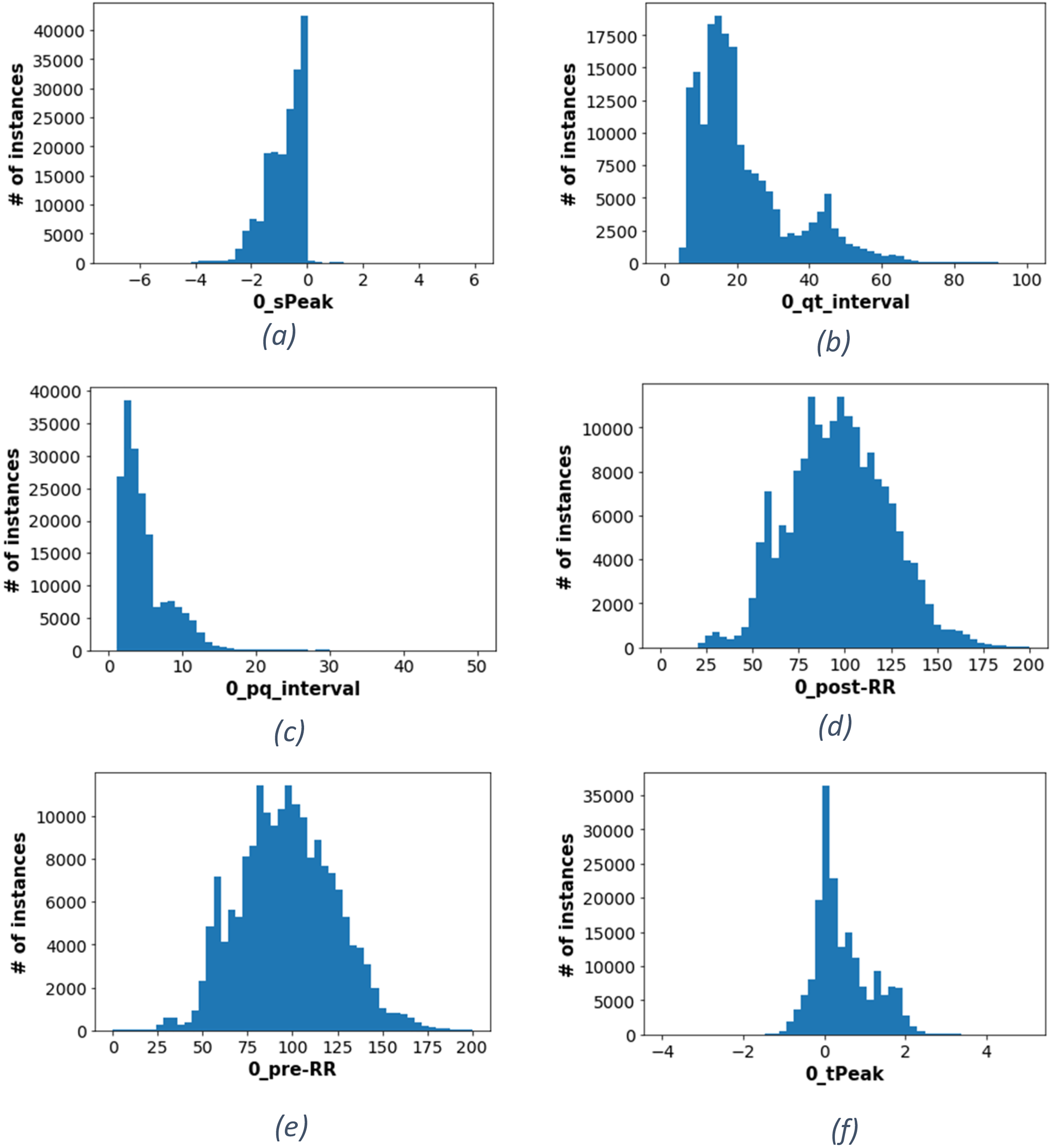
Features distribution (a) histogram of the peak of the S wave (b) histogram of the QT interval (c) histogram of the PQ interval (d) histogram of the post-RR (e) histogram of the pre-RR (f) histogram of the peak of the T wave.

It is important to note that the normal range for the pre-RR and post-RR intervals can vary depending on many factors, including a person's age, gender, and underlying health conditions. That is why they have a more widespread normal distribution, as shown in Figure 2(d) and (e). However, other attributes like the tPeak seem more concentrated within a smaller range, as shown in Figure 2(f).

Figure 3 illustrates the distribution of each class within the base dataset. It can be seen that the classes of the dataset are imbalanced. For example, the F and Q classes constitute 0.012% and 0.043% of the data, respectively. This is significantly lower than the number of instances from other classes, such as the N class, contributing to around 87.913% of the dataset. Such imbalance can lead to poor performance in the less frequently occurring classes since the model may have difficulty learning the characteristics of these minority classes. Moreover, the model's accuracy could be misleading when applied to an imbalanced dataset because it does not consider the recall of rare classes.

Figure 3.

Distribution of classes.

Data pipeline

Figure 4 shows the data pipeline for this work. Once the data is cleaned, it is split into training and testing sets, and each is scaled separately. Since the dataset is unbalanced, the SMOTE balancing technique is used to compensate for the minority classes in the dataset. Afterward, the model is trained and undergoes a series of iterations for hyperparameters turning. Once the model training and optimization are complete, its performance is evaluated on the test dataset. Such a process is a standard practice in any machine learning project.

Figure 4.

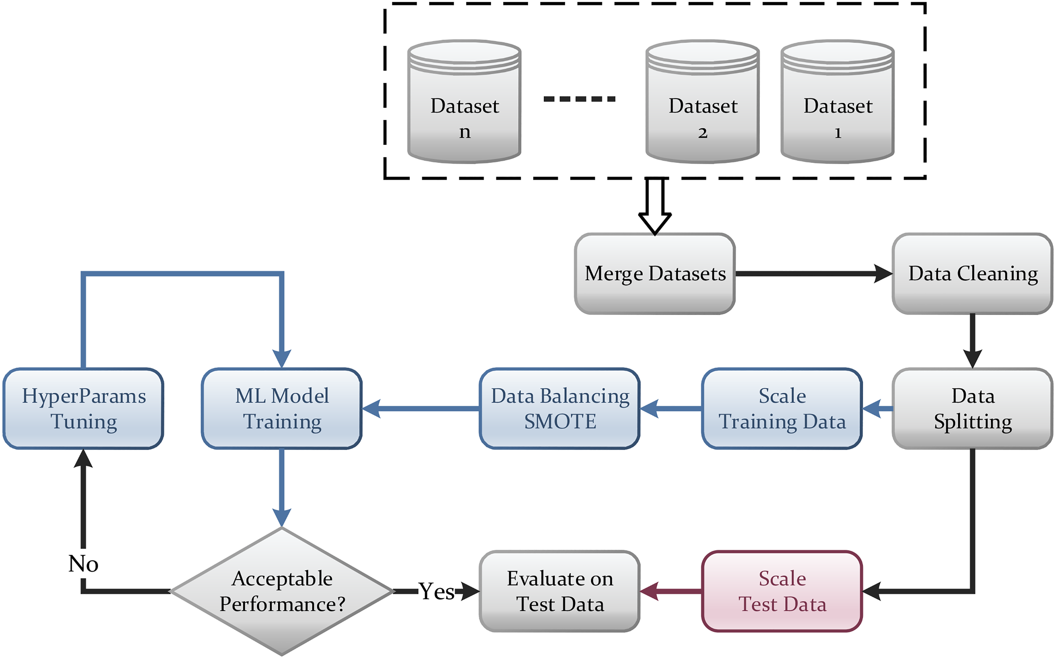
Data pipeline.

Data preprocessing is essential in data analysis because rows are often incomplete, noisy, or inconsistent and may need to be cleaned and transformed before they can be used effectively. For example, the feature “record” was dropped since it only refers to the patient number and does not help predict the type of ECG signal, so it was discarded.

The base dataset is free from noisy rows. However, the values must be scaled for better performance, efficiency, and accuracy. The normalization technique which results in the most significant improvement is the standardization scaling technique. Standardization is often used to scale variables to a common scale because it preserves the shape of the distribution of the data. It can be helpful if the data is not normally distributed and is less sensitive to outliers. The standardization equation is referred to in Equation (1).

X_{S t a n d} = \frac{x - m e a n (x)}{S t a n d a r d D e v i a t i o n (x)}

(1)

Machine learning algorithms

This work will examine several machine learning algorithms to evaluate their performance in the ECG classification problem. As shown in Figure 5, the machine learning models are RF, logistic regression (LR), KNN, linear SVM (LSVM), and linear discriminant analysis (LDA). Any of these models will have hyperparameters that need to be tuned. However, all of them will have the same input features, which are 16 inputs per lead. These are the (p, q, r, s, t) peaks, (pq, qt, st, qrs) intervals, the Pre-RR and post-RR, and the five qrs morphologies. The model will classify any input ECG into one of the five classes N, SVEB, VEB, Q, and F.

Figure 5.

Detailed classification model diagram.

Logistic regression

LR is a type of statistical model that is used for classification tasks. It is called “logistic regression” because it uses a logistic function to predict the probability of an event occurring. It predicts the probability that an ECG signal belongs to a particular class.²⁴

Random Forest

RF is one of the machine learning algorithms used for classification. The basic concept of this algorithm is that it is made of many individual decision trees that work together to make predictions. Each decision tree in an RF is trained on a random subset of the data and makes predictions based on the features of that tree. The predictions from the individual decision trees are then combined to make the final prediction of the RF.²⁵

K-nearest neighbor

The KNN algorithm applies proximity to classify or predict how a single data point will be grouped. It is a nonparametric, supervised learning classifier. It operates under the concept that related points can be discovered close to one another. A class label is chosen by a majority vote, meaning that it chooses the one that is most frequently used in the region of a particular data point.^26,27

Linear support vector machine

LSVM works by finding a hyperplane in a high-dimensional space that maximally separates classes, where the hyperplane is a line that separates the data. Finding a line that perfectly separates linearly separable classes is possible. For nonlinear classes, finding a good separation line is possible by adding additional dimensions and then projecting the data into a higher dimensional space.²⁸

Linear discriminant analysis

LDA is a dimensionality reduction technique. It finds the linear combination of features that maximizes the separation between the different classes. This is done by finding the projection of the data onto a lower-dimensional space. LDA is a supervised method that considers class labels when finding the data projection.²⁹

Results and analysis

This section presents the results on the MIT-BIH supraventricular dataset (the base dataset), then shows the SMOTE technique's impact on enhancing the results. Then shows how combining data from multiple sources enhances the results. Finally, the best results are compared against the latest in the literature.

Base dataset results

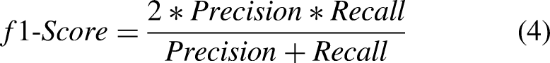
To compare the performance of different models, recall, precision, and F1-scores were used alongside accuracy. Precision is defined as the model's ability to correctly predict the positive class, whereas recall is the ability of the model to identify all positive instances correctly. The primary performance measure used in the comparison in this work is the recall. One would want to detect all types of classes and not miss any. Equations for the precision, recall, F1-score, and specificity are presented in Equations (2)–(5).

P r e c i s i o n = \frac{T P}{T P + F P}

(2)

R e c a l l = \frac{T P}{T P + F N}

(3)

f 1 - S c o r e = \frac{2 * P r e c i s i o n * R e c a l l}{P r e c i s i o n + R e c a l l}

(4)

S p e c i f i c i t y = \frac{T N}{T N + F P}

(5)

Logistic regression

Figure 6(a) shows the confusion matrix of the LR model. No instances are detected as Q or F based on the values provided. Although the test data includes 24 instances labeled as Q and seven instances labeled as F, the model predicts them as N, SVEB, Q, and VEB instead. This shows the model's weakness in detecting Q and F classes, causing the recall to be zero. The accuracy given by this model equals 93%. However, accuracy is not enough indicator of performance for classification models since it does not consider data imbalance. Table 4 shows the overall results of LR.

Figure 6.

Confusion matrix of all algorithms (a) confusion matrix for LR (b) confusion matrix for RF (c) confusion matrix for KNN (d) confusion matrix for LSVM (e) confusion matrix for LDA.

Table 4.

Analysis of LR classifier on original data.

Type	Precision	Recall	F1-score	Specificity
N	95%	98%	97%	59.6%
SVEB	65%	42%	51%	98.4%
VEB	77%	63%	70%	99%
F	0%	0%	0%	100%
Q	0%	0%	0%	100%

SVEB: supraventricular ectopic beat; VEB: ventricular ectopic beat; LR: logistic regression.

Random Forest

RF yields a total accuracy of 98%. As shown in the confusion matrix in Figure 6(b) and Table 5, the model performs better for the F class since it detects two out of seven instances as F, and the recall is equal to 29%. However, the Q class does not improve, with its recall still equal to zero.

Table 5.

Analysis of RF classifier on original data.

Type	Precision	Recall	F1-score	Specificity
N	98%	99%	99%	87.8%
SVEB	91%	80%	85%	99.4%
VEB	95%	92%	93%	99.7%
F	50%	29%	36%	99.9%
Q	0%	0%	0%	100%

SVEB: supraventricular ectopic beat; VEB: ventricular ectopic beat; RF: Random Forest.

K-nearest neighbor

KNN provides an accuracy of 97%. Table 6 provides the recall, precision, F1 score, and specificity of both F and Q classes, which shows better readings than previous algorithms. Moreover, Figure 6(c) shows that two out of seven instances are correctly predicted as F, and only one is detected correctly as Q.

Table 6.

Analysis of KNN classifier on original data.

Type	Precision	Recall	F1-score	Specificity
N	98%	99%	99%	87.3%
SVEB	87%	80%	83%	99.1%
VEB	95%	91%	93%	99.7%
F	67%	29%	40%	99.9%
Q	50%	4%	8%	99.9%

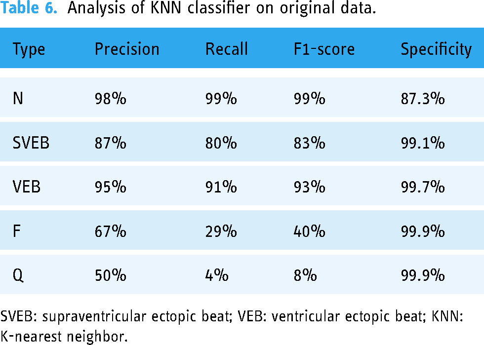
SVEB: supraventricular ectopic beat; VEB: ventricular ectopic beat; KNN: K-nearest neighbor.

Linear support vector machine

The measured accuracy is 92%. Like LR and as shown in Figure 6(d), not a single instance of Q or F is detected. LR produces slightly better results than Linear SVM in terms of accuracy, F1-score, recall, precision, and specificity, as shown in Table 7.

Table 7.

Analysis of LSVM classifier on original data.

Type	Precision	Recall	F1-score	Specificity
N	94%	99%	96%	51%
SVEB	63%	30%	41%	98.7%
VEB	77%	60%	68%	99%
F	0%	0%	0%	100%
Q	0%	0%	0%	100%

SVEB: supraventricular ectopic beat; VEB: ventricular ectopic beat; LSVM: linear support vector machine.

Linear discriminant analysis

The LDA measured accuracy is 92%. As shown in Figure 6(e), all instances of F are predicted as either N or VEB. As for Q, only four instances are correctly predicted. Table 8 illustrates the precision, recall, F1-score, and specificity values.

Table 8.

Analysis of LDA classifier on original data.

Type	Precision	Recall	F1-score	Specificity
N	95%	98%	96%	58.3%
SVEB	60%	39%	47%	98.1%
VEB	74%	62%	67%	98.8%
F	0%	0%	0%	99.9%
Q	4%	17%	6%	99.8%

SVEB: supraventricular ectopic beat; VEB: ventricular ectopic beat; LDA: linear discriminant analysis.

Results using SMOTE technique

The charts in Figure 7 compare the recall of the different models before and after applying data augmentation using SMOTE. Figure 7(a) shows the impact of applying SMOTE on the LR model. While the Q and F classes experienced huge growth, the recall of the N class dropped to 74%. As for the SVEB and VEB, an increase in recall values is detected.

Figure 7.

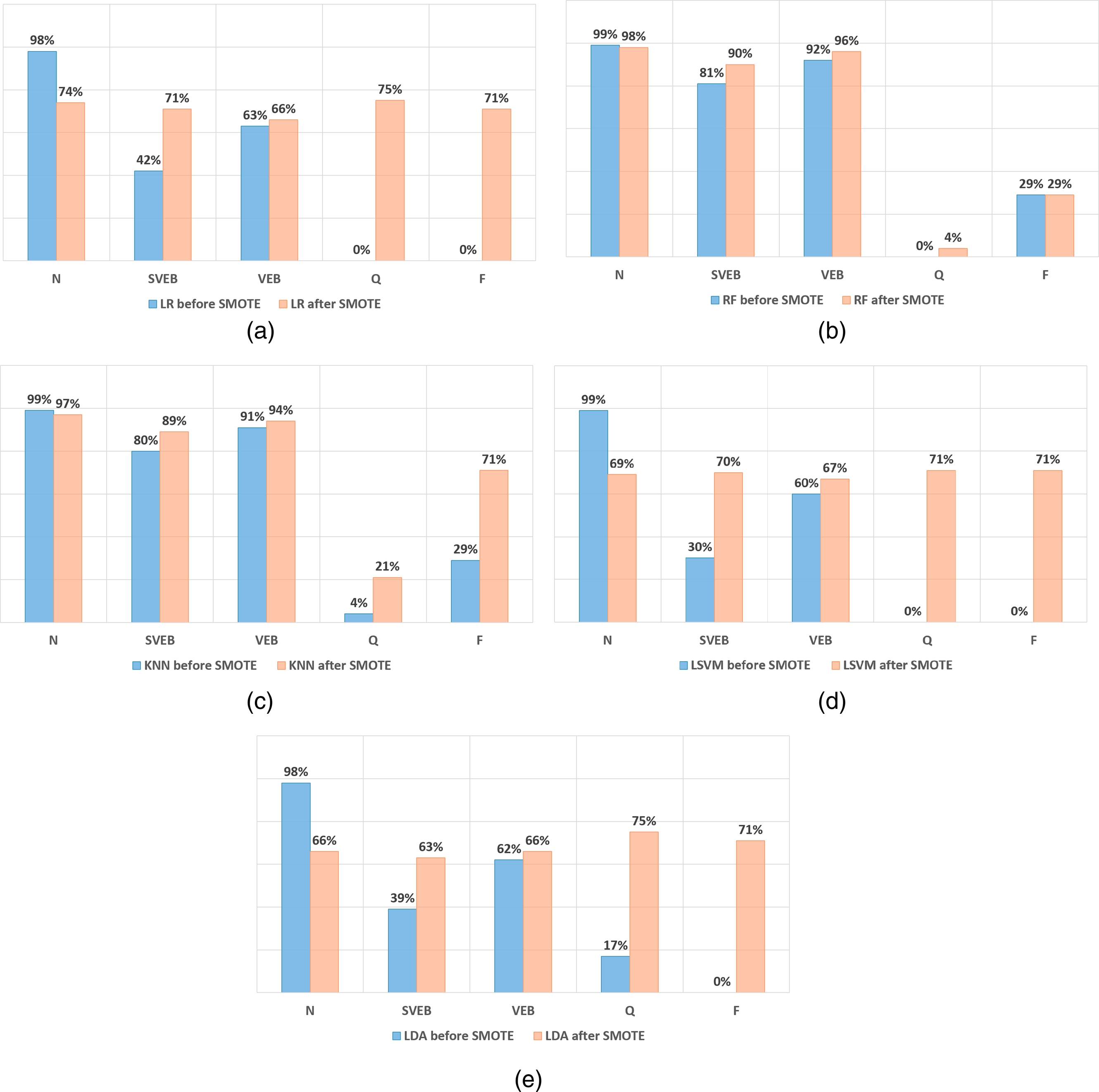
Recall values before and after SMOTE (a) LR (b) RF (c) KNN (d) LSVM (e) LDA.

Figure 7(b) refers to the RF model. After applying SMOTE, there are upward trends in recall in all classes except the N class, which dropped only by 1%, and the F class, which did not change. Overall, the performance of SVEB and VEB is outstanding. However, F and Q did not mark any considerable improvements. The analysis of the KNN model is illustrated in Figure 7(c), where SMOTE clearly shows enhancement in the F class, which increases to 71%, whereas Q increases to 21%. Also, SVEB and VEB classes slightly rise in recall values, yet N decreases by 3% after implementing SMOTE.

Figure 7(d) compares the Linear SVM model. SMOTE causes F and Q classes to rise to 71%. However, this causes a significant fall in the results for the N class, dropping from 99% to 69%. This model is considered weak since all classes have a low recall compared to the previous algorithms. Finally, Figure 7(e) shows information about the LDA model results. Q and F recall increases to more than 70% after SMOTE. Similarly, the SVEB and VEB recall increases slightly to 63% and 66%, respectively. However, the recall of the N class becomes worse than its value before SMOTE.

In summary, SMOTE efficiently improves the recall of the F and Q classes in LR, LSVM, and LDA models. However, the overall performance of all classes is not at its best, as the accuracy drops to 72%, 69%, and 66%, respectively.

Results of using the combined dataset

More F and Q instances are added from different datasets and merged into the base dataset to improve the results further. The new data is cleaned and prepared before merging with the base dataset. This guarantees accurate analysis to compare the results and benchmark the improvements fairly.

Starting with The Sudden Cardiac Death Holter Database,²¹ many instances have features of lead V2 only and instances with features of lead V5 only. For data consistency, instances with missing values from either lead are dropped. The cleaned data is then merged with the clean version of the MIT-BIH arrhythmia dataset¹⁴ and the IN-CART 12-lead Arrhythmia Database.²⁰ However, since the main target is increasing the unique instances for both Q and F classes, instances with class N, VEB, and SVEB are dropped from the merged dataset to diminish the unbalancing that would arise. Finally, the merged dataset is added to the base MIT-BIH supraventricular dataset.

Figure 8 shows the number of the Q and F classes before and after adding the instances from the supplementary datasets. The final distribution of the classes after adding the new instances are added is shown in Figure 9. Then, this new combined dataset is processed using the data pipeline presented earlier, shown in Figure 4, including data splitting, scaling, balancing, and modeling.

Figure 8.

Number of instances of types F and Q before and after adding multiple datasets.

Figure 9.

Percentage of instances after adding multiple datasets.

Figure 10 compares the recall values between those generated using the base dataset and those generated using the combined dataset. It is worth noting that both cases utilized the SMOTE technique to oversample minority classes. Figure 10(a) compares the results for the LR model; it clearly shows that the F class gained the most benefit after merging the datasets as its recall increased to 92%. In contrast, the Q class performed worse after the merge, dropping from 75% to 48%. As for the remaining classes, N and VEB classes showed slight enhancement, while SVEB remained unchanged.

Figure 10.

Recall values of base dataset versus combined dataset both after SMOTE (a) LR (b) RF (c) KNN (d) LSVM (e) LDA.

Figure 10(b) shows a similar comparison for the RF model. The F class shows massive growth, increasing from 29% to 94%. Also, the Q class has improved from 4% to 19%. Moreover, this model did not affect the remaining classes significantly, as they performed well after merging the datasets. Similar results in Figure 10(c) show the comparison for the KNN model, where it shows that recall of F and Q increased to 95% and 26%, respectively, without negatively affecting the remaining classes.

As for Linear SVM, its results are presented in Figure 10(d). Adding more instances for F and Q classes positively affected the recall of the F class. However, Q class recall dropped from 71% to 37%. Generally, this model did not achieve good results for both the base and the merged datasets.

Finally, Figure 10(e) illustrates the results for LDA before and after combining the multiple datasets. Merging the datasets resulted in worse results for all classes except for the N class.

To further analyze the details of these algorithms, the confusion matrices for these algorithms are shown in Figure 11. Among these algorithms, RF and KNN proved to be the most efficient models capable of predicting all classes with the most negligible errors, as shown in Figure 11(b) and (c). They achieved the best recall values for all classes and improved the predictions of the Q and F classes. RF achieved an accuracy of 97%, making it the most reliable classifier that optimized the predictions of the F and Q classes and raised their recall values to 94.4% and 18.5%, respectively. Meanwhile, LSVM, LR, and LDA provided good recall values for the Q and F classes; however, they were excluded from further consideration due to the apparent drop in results for the other classes, as shown in Figure 11(a), (d) and (e). KNN provided good recall values, but after comparing it with RF, it can be seen that RF provides better recall values for N, SVEB, and VEB.

Figure 11.

Confusion matrices of all algorithms using the combined dataset and SMOTE (a) confusion matrix for LR (b) confusion matrix for RF (c) confusion matrix for KNN (d) confusion matrix for LSVM (e) confusion matrix for LDA.

These results demonstrate that the dataset preprocessing using SMOTE and the data-merging techniques have significantly improved the classification models’ performance. And that the RF can provide better classification accuracy for the given dataset.

Finally, the RF model was fine-tuned by altering two hyper-parameters, “n estimators” and “min samples leaf.”³⁰ Figure 12 shows the normalized confusion matrix of the RF classifier, which exceeds the previously reported KNN classifier performance for the Q and F classes. The final performance metrics of the fine-tuned RF model across all classes are provided in Table 9 and Figure 13.

Figure 12.

Confusion matrix of RF model after parameter optimization.

Figure 13.

Analysis of the RF classifier after fine-tuning.

Table 9.

Analysis of the RF classifier after parameter optimization.

Type	Precision	Recall	F1-score	Specificity
N	100%	97%	98%	96.7%
SVEB	71%	93%	80%	97.3%
VEB	92%	95%	93%	99.5%
F	98%	95%	96%	100%
Q	19%	30%	23%	100%
Accuracy	97%

SVEB: supraventricular ectopic beat; VEB: ventricular ectopic beat; RF: Random Forest.

In conclusion, considering all results, the most efficient models that proved their capability of predicting all classes with the least errors were RF and KNN after applying SMOTE on the merged dataset since they achieved the best recall values for all classes and improved the predictions of Q and F classes. Looking for the best accuracy, RF achieved an accuracy equal to 97%. However, KNN recorded 96%. Thus, RF is considered the most reliable classifier, which optimized the predictions of F and Q classes and raised their recall values to 95% and 30%, respectively. Thus, it will be selected for comparison against other works in the literature.

Results comparison with literature

To compare the obtained results with previous related work, Table 10 shows the recall values of the five classes for this work and four leading research papers. Considering the recall of the F class, it can be seen that in this work, it is 95% exceeding the 93.8% reported by Zhang et al.¹⁵

Table 10.

Comparison of recall and accuracy with other papers.

Type	This work	Zhang et al.¹⁵*	Bhattacharyya et al.¹⁸	T. Wang et al.¹³*	L. Wang et al.¹⁹
N	97%	88.9%	99.5%	91.7%	96.37%
SVEB	93%	79%	74.2%	89.9%	80.47%
VEB	95%	85.4%	94.2%	87.8%	96.99%
F	95%	93.8%	73.2%	55.4%	22.75%
Q	30%	0%	0%	0%	8.33%
Accuracy	97%	86.6%	98.2%	95.6%	94.4%

Moreover, the Q class has the highest percentage at 30% in this work, while others reported 0% in this category, and¹⁹ has the highest percentage among the four individuals at 8.33%. Notably, works denoted with (*) chose to drop all Q instances from their datasets. But in this work, adding multiple datasets and implementing data augmentation could improve the recall to 30%, as shown in Figure 14, without affecting the remaining classes. Besides that, better results were achieved even for SVEB class. While it is true that the performance of work¹⁹ outperformed our results by around 2% in the specific VEB category, it is essential to note that the performance of the remaining classes was worse than what this work achieved. Taking accuracy into consideration, work in Bhattacharyya et al.¹⁸ achieved better accuracy. However, accuracy was sacrificed to enhance the predictions of F and Q that were neglected in most papers.

Figure 14.

Comparison of recall values with other papers.

Conclusion

In summary, this article aimed to build an ECG heartbeat classification model with an enhancement to the Recall values of types F and Q without affecting the recall of the other types. After comparing five different supervised machine-learning algorithms on the base dataset, SMOTE technique was implemented on the five models, and their results were compared. It was noticeable that for most models, the recall for types N, SVEB, and VEB was much higher than for types F and Q. As such, instances of types F and Q from three other datasets were combined with the base dataset. SMOTE was then implemented to balance the data as a further enhancement, and the results were reevaluated. It was concluded that the RF model after SMOTE was implemented had the best overall results considering that the accuracy remained high and the recall for all types increased. This final model provided an accuracy of 97% and a recall of 97%, 93%, 95%, 95%, and 30% for types N, SVEB, VEB, F, and Q, respectively.

The clinical application of such a model would be having physicians in remote areas analyze the ECGs quickly without needing a cardiologist for every ECG analysis. A practical deployment of this machine-learning model can be done by adding a processing layer to capture a single heartbeat, extracting the required parameters from the heartbeat, then feeding them into the machine-learning model for classification. The model can be installed on IoT devices and provide preliminary classification (diagnosis), saving time and lives. While the scope of this work focused on the machine learning part, building a fully functional prototype could be considered in future work.

Footnotes

Acknowledgements

Not Applicable.

Contributorship

Amjed Al-Mousa provided a continuous review of the means and methods used, revised the manuscript several times, and prepared the final version, which was approved by all authors. Joud Baniissa, Tala Hashem, and Tala Ibraheem contributed to conceptualization, conducted the literature review, and contributed to data preparation and code implementation.

Declaration of conflicting interests

The author(s) declared no potential conflicts of interest with respect to the research, authorship, and/or publication of this article.

Funding

The author(s) received no financial support for the research, authorship, and/or publication of this article.

Ethical approval

This work did not involve any human or animal trials. The datasets used in this work are anonymous and available in the public domain.

Consent statement

Patient consent is not applicable in this research, as there has been no human or animal testing involved.

Guarantor

Amjed Al-Mousa.

ORCID iD

Amjed Al-mousa

References

WHO. WHO reveals leading causes of death and disability worldwide: 2000–2019. 12 2020. [Online], https://www.who.int/news/item/09-12-2020-who-reveals-leading-causes-of-death-and-disability-worldwide-2000-2019.

Mayo Clinic. Heart arrhythmia. 2023. [Online], https://www.mayoclinic.org/diseases-conditions/heart-arrhythmia/symptoms-causes/syc-20350668.

Mayo Clinic. Cardiac Abalation. 2023. [Online], https://www.mayoclinic.org/tests-procedures/cardiac-ablation/about/pac-20384993.

Rai

Chatterjee

. Hybrid CNN-LSTM deep learning model and ensemble technique for automatic detection of myocardial infarction using big ECG data. Appl Intell 2022; 52: 5366–5384.

Rai

Chatterjee

. A unique feature extraction using MRDWT for automatic classification of abnormal heartbeat from ECG big data with multilayered probabilistic neural network classifier. Appl Soft Comput 2018; 72: 596–608.

Rai

Chatterjee

. A novel adaptive feature extraction for detection of cardiac arrhythmias using hybrid technique MRDWT & MPNN classifier from ECG big data. Big Data Research 2018; 12: 13–22.

American National Standard. Testing and reporting performance results of cardiac rhythm and ST segment measurement algorithms. Association for the Advancement of Medical Instrumentation. 2013.

Greenwald

. Improved detection and classification of arrhythmias in noise-corrupted electrocardiograms using contextual information . Massachusetts, USA: Harvard University–MIT Division of Health Sciences and Technology, 1990

Abdulhadi

Al-Mousa

. Diabetes detection using machine learning classification methods. In: 2021 international conference on information technology (ICIT), Amman, 2021.

10.

Atallah

Al-Mousa

. Heart disease detection using machine learning majority voting ensemble method. In: 2019 2nd international conference on new trends in computing sciences (ictcs), 2019.

11.

Jahed

Aseer

Al-Mousa

. Using personal key indicators and machine learning-based classifiers for the prediction of heart disease. In: international conference on smart computing and application (ICSCA), Hail, Saudi Arabia, 2023.

12.

Al-Zubaidi

Dweik

Al-Mousa

. Stroke prediction using machine learning classification methods. In: international arab conference on information technology (ACIT), Abu Dhabi, UAE, 2022.

13.

Wang

, et al. Imbalanced heartbeat classification using EasyEnsemble technique and global heartbeat information. Biomed Signal Process Control 2022; 71: 1.

14.

Moody

Mark

. The impact of the MIT-BIH arrhythmia database. IEEE Eng Med Biol Mag 2001; 20: 45–50.

15.

Zhang

Dong

Luo

, et al. Heartbeat classification using disease-specific feature selection. Comput Biol Med 2014; 46: 79–89.

16.

Dıker

Avci

Cömert

, et al. Classification of ECG signal by using machine learning methods. In: 2018 26th signal processing and communications applications conference (SIU), 2018.

17.

Alarsan

Younes

. Analysis and classification of heart diseases using heartbeat features and machine learning algorithms. J Big Data 2019; 6: 1–15.

18.

Bhattacharyya

Majumder

Debnath

, et al. Arrhythmic heartbeat classification using ensemble of random forest and support vector machine algorithm. IEEE Trans Artificial Intell 2021; 2: 260–268.

19.

Wang

L-H

Y-T

Liu

, et al. Three-Heartbeat multilead ECG recognition method for arrhythmia classification. IEEE Access 2022; 10: 44046–44061.

20.

Yakushenko

. St Petersburg INCART 12-lead arrhythmia database. 2008.

21.

Greenwald

. The development and analysis of a ventricular fibrillation detector . Massachusetts, USA: Massachusetts Institute of Technology, 1986

22.

Hampton

. The ECG made easy. Amsterdam, Netherlands: Elsevier, 2019.

23.

Ahmed

Haskell-Dowland

. Secure edge computing: applications, techniques and challenges. Florida, USA: CRC Press, 2021.

24.

Sammut

Webb

(eds). Logistic regression. Encyclopedia of machine learning. Boston, MA: Springer, 2010, pp.631–631.

25.

Breiman

. Random forests. Mach Learn 2001; 45: 5–32.

26.

Zhang

. Introduction to machine learning: k-nearest neighbors. Ann Transl Med 2016; 4: 2–3.

27.

Harrison

. Machine learning basics with the k-nearest neighbors algorithm. 2018. [Online], https://towardsdatascience.com/machine-learning-basics-with-the-k-nearest-neighbors-algorithm-6a6e71d01761.

28.

Zhang

. Support vector machines. In: Sammut

Webb

(eds) Encyclopedia of machine learning, Boston, MA: Springer US, 2010, pp.941–946.

29.

Izenman

. Linear discriminant analysis. In: Allen

De Veaux

Nugent

(eds) Modern multivariate statistical techniques: regression, classification, and manifold learning. New York, NY: Springer New York, 2008, pp.237–280.

30.

Arya

. Tuning Random Forest Hyperparameters. 8 2022. [Online], https://www.kdnuggets.com/2022/08/tuning-random-forest-hyperparameters.html (accessed 13 May 2023).

Enhanced electrocardiogram machine learning-based classification with emphasis on fusion and unknown heartbeat classes

Abstract

Keywords

Introduction

Related work

Dataset and experimental setup

Datasets

Data attribute information

Data pipeline

Machine learning algorithms

Logistic regression

Random Forest

K-nearest neighbor

Linear support vector machine

Linear discriminant analysis

Results and analysis

Base dataset results

Logistic regression

Random Forest

K-nearest neighbor

Linear support vector machine

Linear discriminant analysis

Results using SMOTE technique

Results of using the combined dataset

Results comparison with literature

Conclusion

Footnotes

Acknowledgements

Contributorship

Declaration of conflicting interests

Funding

Ethical approval

Consent statement

Guarantor

ORCID iD

References