Sage Journals: Discover world-class research

Abstract

The temporal relationship between changes in cerebral blood flow (CBF) and cerebral blood volume (CBV) is important in the biophysical modeling and interpretation of the hemodynamic response to activation, particularly in the context of magnetic resonance imaging and the blood oxygen level–dependent signal. Grubb et al. (1974) measured the steady state relationship between changes in CBV and CBF after hypercapnic challenge. The relationship CBVαCBF^Φ has been used extensively in the literature. Two similar models, the Balloon (Buxton et al., 1998) and the Windkessel (Mandeville et al., 1999), have been proposed to describe the temporal dynamics of changes in CBV with respect to changes in CBF. In this study, a dynamic model extending the Windkessel model by incorporating delayed compliance is presented. The extended model is better able to capture the dynamics of CBV changes after changes in CBF, particularly in the return-to-baseline stages of the response.

Keywords

Dynamic modeling Cerebral blood flow Cerebral blood volume Balloon Windkessel Delayed compliance

Roy and Sherrington (1890) proposed that increases in neural activity, metabolism, and blood flow were tightly linked. However, the precise nature of the temporal relationship between the changes in cerebral blood volume (CBV) and CBF, an elemental aspect of neurovascular physiology, is still poorly understood. With the developments of functional magnetic resonance imaging (fMRI), and particularly in the increasing use of brief-duration transient stimuli in event-related studies, it is becoming increasingly important to clarify the temporal dynamics of the relationship. The blood oxygen level–dependent (BOLD) signal is the image contrast commonly used in human fMRI studies resulting from a complex interplay of blood volume, flow, and increases in oxygen consumption (Jones et al., 2001). In our study, changes in CBV were measured by optical imaging spectroscopy (OIS) and changes in CBF were measured using laser-Doppler flowmetry (LDF).

The relationship between changes in blood flow (volume flux per unit time through a tissue volume element) and volume was first established by Grubb et al. (1974). It was found that volume changes followed flow changes raised to an exponent and the power relationship CBVαCBF^0.38 has been used extensively in the modeling of the hemodynamic response to activation (Buxton et al., 1998; Mandeville et al., 1999). However the relationship was based on ‘steady state’ measurements, and its generalization to activation paradigms involving transient changes is not established.

A biomechanical model (the Balloon model) was introduced by Buxton et al. (1998). This model assumes that the volume changes occur primarily in the venous compartment, and the rate of change is proportional to the difference between the inflow and outflow of the compartment with a time constant. Mandeville et al. (1999) modeled the dynamics of the relationship in terms of the resistance and capacitance of the venous and capillary microvasculature (Windkessel theory). In addition they noted that different time constants were necessary to model explicitly in time the increase and the return-to-baseline phases of the changes in CBF and CBV, but this would require an unspecified mechanism to switch between them in the model. However, a modification of the Windkessel model to include an additional state variable incorporating delayed compliance is better able to describe these aspects of the dynamics of CBV changes in relation to CBF changes.

MATERIALS AND METHODS

Experimental data

The two data sets presented here are reworked from Jones et al. (2002) and Martindale et al. (2003). The experimental procedures for concurrent measurement of volume and flow changes are described in greater detail in Jones et al. (2002). They are briefly reviewed here.

The animals used were Hooded Lister rats weighting between 300 and 400 g, anesthetized with urethane (1.25 g/kg, intraperitoneal injection), and atropine (0.4 mL/kg, subcutaneous injection). The first stage is to locate a whisker barrel using single-wavelength (~590 nm) illumination, and then the slit spectrograph mounted on the camera is appropriately sited over the center of the barrel region. Spectroscopic data were analyzed using a path length–scaling algorithm (Mayhew et al., 1998). After placement of the spectrograph, an LDF probe (Perimed, Stockholm, Sweden; fiber separation 0.25 mm) is placed over the barrel region (<1 mm from skull surface) to measure flow changes. The LDF spectrometer includes a lowpass filter with a 0.2-second time constant and 12-kHz bandwidth (Nilsson, 1984) to reduce errors caused by measurement noise. The LDF time series were collected concurrently with spectrographic data for each of the following conditions:

•

Long stimulation (n = 6). The stimulation of somatosensory cortex used electrical simulation of the whisker pad at three levels of intensity (0.8, 1.2, and 1.6 mA at 5 Hz). Each trial lasted 50 seconds with the stimulus onset at 10 seconds with a 20-second duration. An intertrial period of 55 seconds between each trial minimized any hemodynamic refractory effects. Data were averaged over 15 trials.

•

Short stimulation (n = 5). The brief (2-second) stimulation was at frequencies of 1, 2, 3, 4, and 5 Hz with an intensity of 1.2 mA. Each trial lasted 23 seconds with stimulus onset at 8 seconds. An intertrial period of 25 seconds was provided between each trial. Data were averaged over 30 trials.

TABLE 1.

Estimated parameters using the Windkessel model (γ) and the MWMC (α and τ) for long-stimulation data sets

	Intensity (mA)
Parameter	0.8	1.2	1.6	Overall

γ Mean (SD)	4.5 (2.7)	3.9 (2.8)	4.1 (2.6)	4.1 (2.5)
α Mean (SD)	4.1 (2.7)	3.8 (2.8)	3.9 (2.5)	3.9 (2.5)
τ_c (s) Mean (SD)	6.7 (2.7)	5.6 (4.4)	10.2 (6.3)	7.5 (4.8)
No. of animals	5	5	5	15

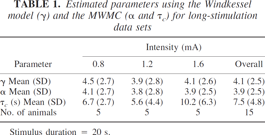
Stimulus duration = 20 s.

The OIS data were captured at 7.5 Hz, and the LDF data were captured at 30 Hz and subsampled to 7.5 Hz. These data are represented as normalized changes from the baseline value,

v = \frac{V}{V_{0}}

and

f = \frac{F}{F_{0}}

(subscript zero denotes the baseline value) are the normalized CBV and CBF changes, respectively.

In our study, OIS has been used to measure changes in oxygenated hemoglobin (HbO₂) and deoxygenated hemoglobin (Hbr), where the total hemoglobin content (Hbt) is given by Hbt = HbO₂ + Hbr. We make the assumption that the overall hematocrit in the sampled cortical volume (~500³ μm) of the measurements remains constant and the changes in CBV are proportional to the change in Hbt, i.e.,

\frac{V}{V_{0}} = \frac{H b t}{H b t_{0}^{.}}

In support, although Schulte et al., (2003) reported some changes in hematocrit in capillaries near the cortical surface (50 to 70 μm) after direct cortical electrical stimulation at high intensities, at peripheral stimulation intensities commensurate with those used in this study, Kleinfeld et al. (1998) found no evidence for increases in capillary hematocrit.

Figures 1a and 1c show the time series of the mean normalized CBF and CBV changes in animals subjected to long periods of electrical stimulation as measured by OIS and LDF, respectively. Figures 1b and 1d show the mean value and standard deviation for CBF and CBV at the time of peak (14.5 seconds for long stimulation). Corresponding figures for the short-stimulation condition are shown in Fig. 2 (time of peak is 11 seconds for short stimulation). It can be seen that the standard deviations are relatively large across animals. This is due largely to the differences between subjects in terms of the magnitude of the responses. Hence, individual subject data will be used in the following sections.

Fig. 1.

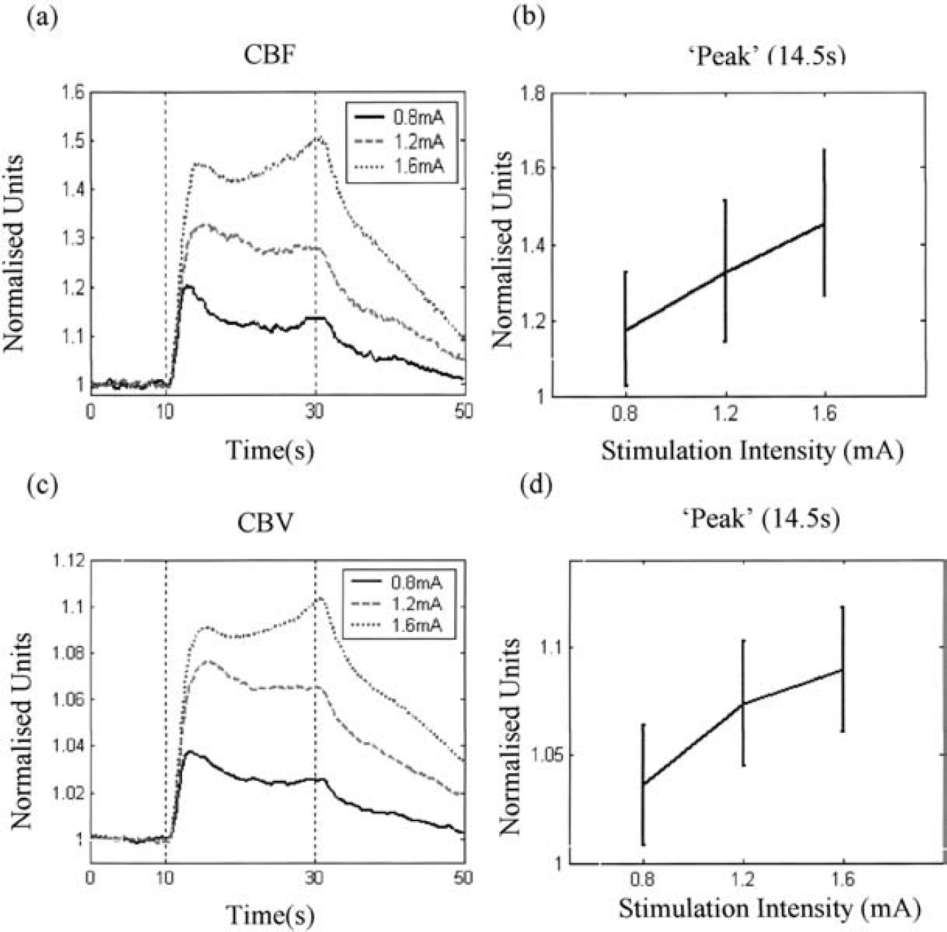
Normalized time series of CBF and CBV to long electrical stimulation. (a) CBF and (c) CBV collected under three levels of stimulation intensities (0.8, 1.2, and 1.6mA). Data are the mean values of six subjects. The mean value and the standard deviation for (b) CBF and (d) CBV for each intensity at the time of peak (14.5 seconds).

Fig. 2.

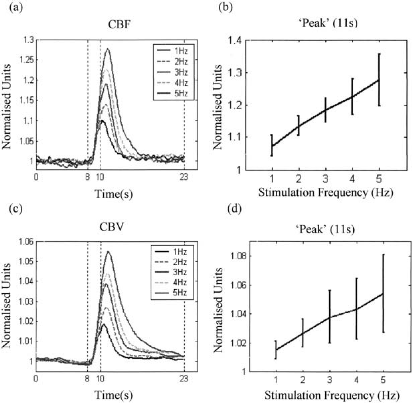
Normalized time series of CBF and CBV to short electrical stimulation. (a) CBF and (c) CBV collected under five levels of pulse frequency (1, 2, 3, 4, and 5 Hz). Data are the mean values of five subjects. The mean value and the standard deviation for (b) CBF and (d) CBV for each intensity of five subjects. The mean value and the standard deviation for (b) CBF and (d) CBV for each frequency at the time of peak (11 seconds).

The condition common to the two experiments (long and short stimulation) used stimulation with an intensity of 1.2 mA at a frequency of 5 Hz. Figures 3a and 3b show the normalized CBF and CBV under this common stimulation condition. It can be seen that the initial dynamic responses are very similar, although the maximum response is larger for long stimulation than for short stimulation for both CBF and CBV changes.

Fig. 3.

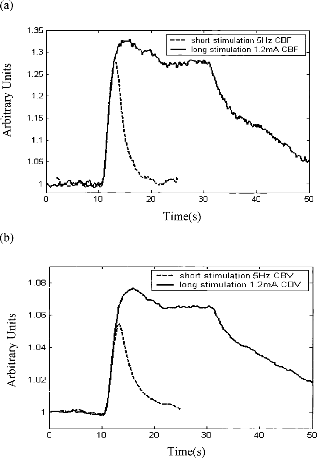
Comparison of the time series f and v under the same stimulus condition (1.2 mA at 5 Hz). (a) The time series f under short stimulation (5 Hz, dashed line) and long stimulation (1.2 mA, solid line). (b) The time series v under short stimulation (5 Hz, dashed line) and long stimulation (1.2 mA, solid line).

Balloon and Windkessel models

Figure 4 shows for comparison the time series of CBF and CBV normalized to within the range of 0 to 1 with respect to the baseline and peak values. The two time series are very similar in shape after the onset of stimulation before the stimulus was withdrawn, indicating that the volume increase has roughly the same time constant as that of the flow. However, the volume returns to baseline at a much slower rate than does the flow. This temporal mismatch between flow and volume changes, also known as the delayed compliance due to circumferential stress relaxation in large blood vessels, has been previously reported by Buxton et al. (1998) and has been used to explain the BOLD poststimulus undershoot, a common phenomenon in fMRI activation studies. Therefore it is important that the model of the dynamic relationship between changes in flow and volume captures this temporal mismatch appropriately.

Fig. 4.

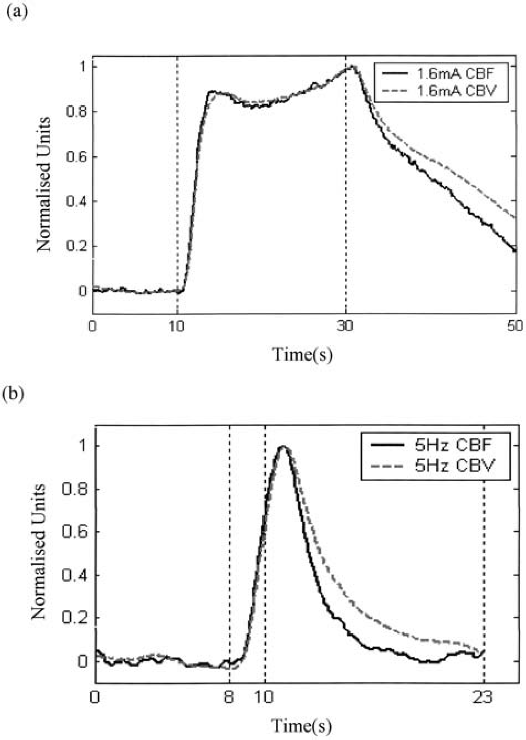
Comparison of f and v normalized to within the range of 0~1 under (a) long stimulation (1.6 mA) and (b) short stimulation (5 Hz).

The relationship between the normalized changes of blood flow and volume, established by Grubb et al. (1974), is

v = \int^{Φ}

(1)

where Φ = 0.38. However different studies have shown that the values of Φ can vary between 0.18 and 0.35 during brief stimulation (Jones et al., 2001, 2002; Mandeville et al., 1998, 1999), which suggests that the relationship proposed by Grubb et al. (based on steady-state measurements) does not capture the complexity of the flow–volume relationship in dynamic conditions.

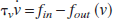
A biomechanical model (the Balloon model; Buxton et al., 1998) relates the changes in volume (v) in a compliant compartment to the difference between inflow (f_in) and outflow (f_out) of that compartment with a time constant τ_v (average venous transit time):

TABLE 2.

Estimated parameters using the Windkessel model (γ) and the MWMC (α and τ_c) for short-stimulus data sets

	Frequency (Hz)
Parameter	1	2	3	4	5	Overall

γ Mean (SD)	6.2 (0.9)	5.4 (1.5)	5.7 (2.1)	5.6 (2.6)	4.9 (1.6)	5.5 (1.6)
α Mean (SD)	5.4 (1.0)	4.4 (1.3)	4.7 (2.1)	4.6 (2.5)	4.0 (1.4)	4.6 (1.6)
τ_c (s) Mean (SD)	2.7 (2.4)	3.4 (1.8)	2.9 (0.6)	3.3 (0.3)	3.7 (1.2)	3.2 (1.4)
No. of animals	4	4	4	3	5	20

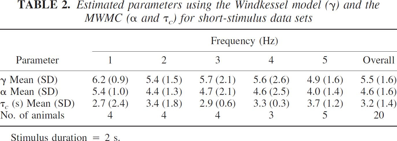
Stimulus duration = 2 s.

τ_{v} \dot{v} = f_{i n} - f_{o u t} (v)

(2)

where f_out(v) is related to v by the relationship proposed by Grubb et al.: f_out(v) = v^1/Φ. This model is a nonlinear first-order system. Implementation shows that it cannot model the slow return-to-baseline behavior of the blood volume, and although Buxton et al. (1998) comment on this and, in their simulations, modeled f_out(v) as the sum of a linear component and a power law, the explicit functional form of f_out(v) was not given.

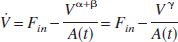
Mandeville et al. (1999) formulated the dynamic relationship between flow and volume in terms of resistance and capacitance (Windkessel theory), which can be written as

\dot{V} = F_{i n} - \frac{V^{α + β}}{A (t)} = F_{i n} - \frac{V^{γ}}{A (t)}

(3a)

where γ = α + β (c.f. Eq. 3 in Friston et al., 2000) and A(t) is a time variable related to the delayed compliance. In their simulations, Mandeville et al. (1999) modeled the delayed compliance term A(t) as an exponential function, and though they “adjusted the time constant and offset to reproduce the data,” they did not enlarge on the details or show how the full dynamic compliance model fitted their data. Equation 3a can be written in normalized terms as

τ_{v} \dot{v} = f_{i n} - \frac{v^{γ}}{A (t)}

(3b)

where a(t) = A(t)/A(0). At steady state under the assumption that the delayed compliance variable is constant, i.e., a(t) = 1, the normalized flow and volume is related by f_in = v^γ, which agrees with the empirical results from Grubb et al.'s relationship.

Furthermore, a distinction must be drawn between the time constants used to parameterize their dynamic model and the exponential time constants used to fit the initial and later stages of the flow and volume time-series data. In what follows, we attempt to extend the Windkessel model by replacing the delayed compliance component a(t), which is an explicit function of time, by a state variable and estimating its temporal evolution using concurrent volume and flow measurements.

Modified Windkessel model with compliance

The delayed compliance is modeled by introducing a normalized state variable c with a time constant τ_c as

τ_{c} \dot{c} = v^{β} - c

(4a)

where at baseline condition, c(0) = 1. Substituting c into Eq. 3b gives

τ_{v} \dot{v} = f_{i n} - \frac{v^{α + β}}{c}

(4b)

Comparing with Eq. 2, we note that f_out is now related to v and c by

f_{o u t} = \frac{v^{α + β}}{c}

(4c)

The model defined by Eqs. 4a–4c is now a second-order nonlinear system. The two time constants needed to capture the dynamics during the different phases of the blood volume changes are now integrated into a model of the flow-to-volume coupling.

Immediately after the onset of the stimulus, if τ_c ≫ τ_v, c will increase slowly from its initial condition of unity and will have little effect on the system dynamics at this stage. The behavior of the system will be therefore very similar to that of the Windkessel model (i.e., f_out and v are mainly related by the power law). At steady state, c = v^β therefore f_out = v^α and Grubb et al.'s relationship holds. When the stimulation ceases, c will return to its baseline slowly (τ_c ≫ τ_v), but because f_out is governed by the first-order system (Eqs. 4b and 4c) with faster time constant τ_v, f_out has to follow f_in, hence returning to its baseline much faster than c. Now we have the situation

f_{o u t} = \frac{v^{α + β}}{c}

Sensitivity analysis

In the analysis of dynamic systems, it is important to characterize the variation in the solutions with respect to variation in the values of the system parameters (Bassingthwaighte and Chaloupka, 1984). Sensitivity analysis makes explicit the dependence of the model on each parameter and the degree to which the parameters are mathematically independent.

S_{p} (t) = \frac{\partial {\overset{\circ}{h}}_{p} (t)}{\partial p} \approx \frac{Δ h_{p} (t)}{Δ p}

Following Bassingthwaighte and Chaloupka (1984), the sensitivity function of a parameter p is defined as where ĥ_p (t) is the analytic impulse response of the model and h_p(t) is the computed impulse response of the dynamic system. For the numerical calculations we describe later, the parameter values were perturbed by 1%. If two parameters are highly correlated, one parameter is usually set to a sensible fixed value. Figure 5 shows the normalized sensitivity functions of the four parameters α, β, τ_v, and τ_c in the modified Windkessel model with compliance (MWMC). It can be seen that the sensitivity functions of α and β are almost identical. Because the steady-state relation is determined by α, it was allowed to vary in the optimizations procedure, and the parameter β was fixed at a value determined by experiment (see Results).

Fig. 5.

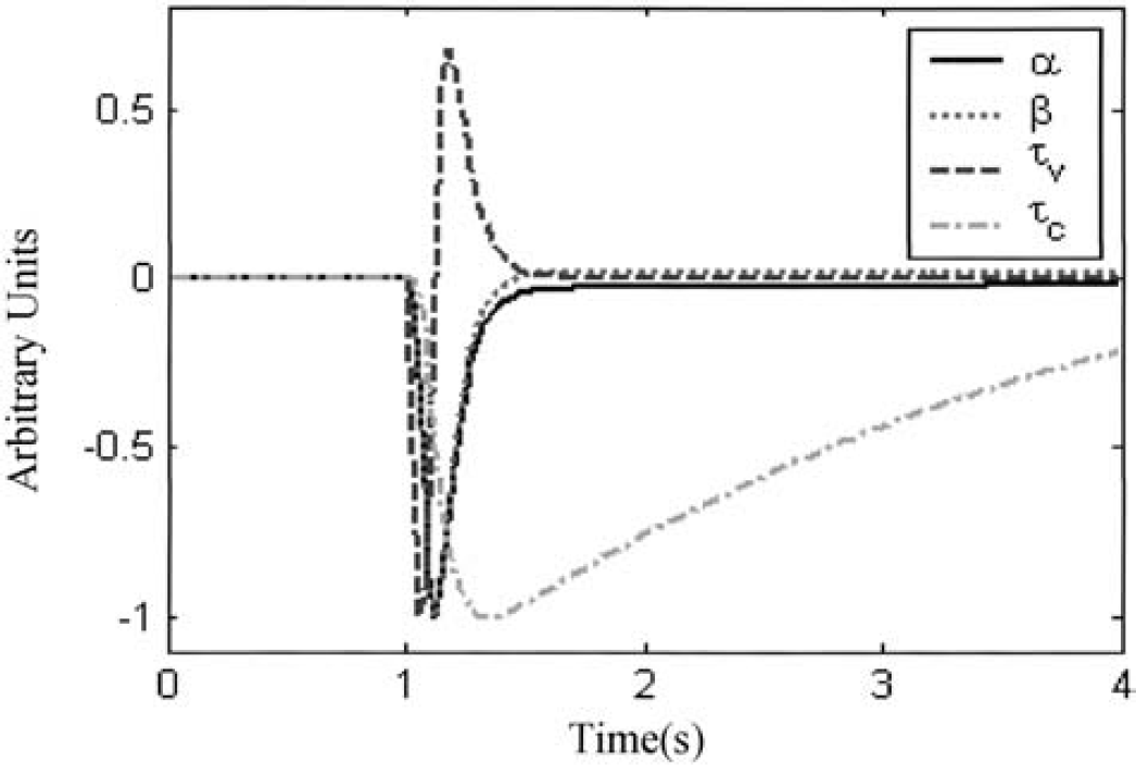
Sensitivity functions for the four parameters in the MWMC, each scaled to have a minimum of −1.

RESULTS

The experiments described here comprised long stimulation (n = 6) and short stimulation (n = 5) data sets. Each individual animal data set was modeled using Mandeville's version of the Windkessel model (Eq. 3b) with the delayed compliance being assumed constant [a(t) = 1] and our modified model with added compliance (Eq. 4). The measured normalized flow (f) was used as input to the system, and the predicted normalized volume (v) as output was compared with the measured volume. The parameters of the two models were estimated using nonlinear least squares (Levenberg-Marquardt algorithm, MATLAB function “lsqnonlin”).

Preliminary analysis showed that both models were insensitive to changes in the values of the parameter τ_v (representing the venous transit time) over the range of values 0.1 to 0.5 seconds; hence, τ_v was fixed at a physiologically plausible value of 0.3 seconds (Nakagawa et al., 1995; Zheng et al., 2002). From the sensitivity analysis, we know that β should be clamped. To choose the appropriate value for β we conducted an exploratory optimization analysis (over all individual data sets), allowing β to vary over the range of 0.1 to 2.6, and found that the minimum prediction error in the least-squares sense was obtained with a β of 1.6 for short-stimulation data and a β of 0.7 for long-stimulation data, and these values were used in the subsequent analysis. For some animals, on some conditions there was little or no evidence of any compliance in the time series of the blood volume. This was revealed in the analysis by a very large value for the compliance time constant τ_c. These conditions were excluded in the calculation of the means and standard deviations of the model parameters (α and τ_c).

Tables 1 and 2 show the optimized values for the parameters (mean and standard deviation) for both the long and short stimulation conditions respectively. The parameters γ and α represent the steady-state relationship between flow and volume of the Windkessel model and the MWMC; hence, they are expected to be similar for the long-stimulus condition. From Table 1, we see that γ and α are indeed similar, but α is consistently smaller than γ. In fact, this was the case for every animal. For the short-stimulus data, the response does not reach a steady state, and the dynamics of the system are determined by the interaction of the parameters α and β and the time constant τ_c. Thus, the parameter α would not be expected to correspond to the value of the parameter γ in the Windkessel model. From Table 2 it can be seen that compared with the long-stimulation condition, the difference between γ and α is much larger for the short-stimulation condition.

Furthermore, for both data sets there is little difference in the range of values of γ and α in either the case of the different intensities (long stimulation; Table 1) or different frequencies (short stimulation; Table 2). The mean of the values of the compliance term τ_c is larger for the long-stimulation condition (7.5 seconds) than for the short-stimulation condition (3.2 seconds). Note that the values of γ and α are larger than the value of 2.63 characteristically associated with Grubb et al.'s relationship.

Figures 6 and 7 show, for comparison, the time series of the normalized volume measurements and the predictions from the models for the long- and short-stimulation conditions, respectively, for a representative animal. In each figure, the solid line represents the original data, the dashed line represents the prediction of the Windkessel model, and the dotted line represents the prediction of the MWMC.

Fig. 6.

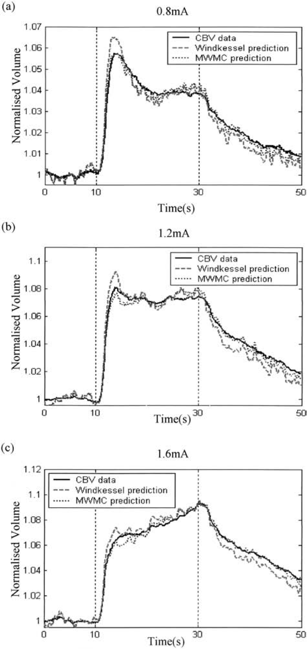
Comparison of the predicted CBVs from the Windkessel model and the MWMC for the long-stimulation condition at different intensities (0.8, 1.2, and 1.6 mA). In each figure, the solid line is the measured data, the dashed line is the predicted CBV from the Windkessel model, and the dotted line is predicted CBV using the MWMC.

Fig. 7.

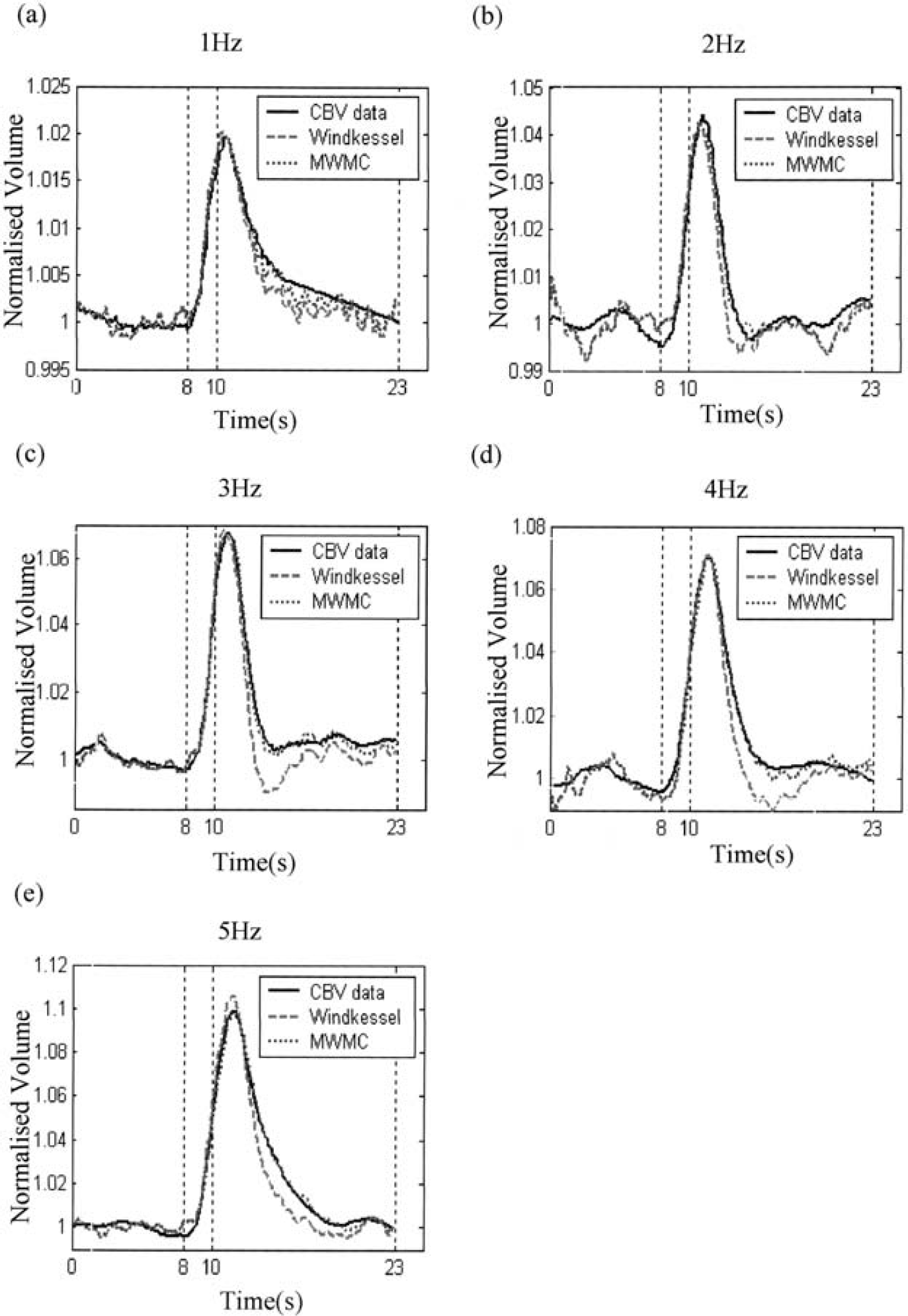
Comparison of the predicted CBVs from the Windkessel model and the MWMC for the short-stimulation condition at frequencies of 1 to 5 Hz. In each figure, the solid line is the measured data, the dashed line is the predicted CBV from the Windkessel model, and the dotted line is predicted CBV using the MWMC.

It can be seen that although the Windkessel model fits the early stages of the experimental data, the predicted time series returns to baseline much faster than the data over the latter stages of the response. In contrast, the MWMC gives excellent predictions over the whole time series including the return-to-baseline stage for all stimulation conditions.

Figures 8 and 9 show the residuals of the predictions for the Windkessel and the MWMC models. It can be seen clearly that model prediction residuals of the MWMC are much smaller than those of the Windkessel model, especially after stimulus cessation and the return-to-baseline stages of the response. Figures 10a and 10b show the histograms of the standard deviation of model prediction residuals over all intensities for the long-stimulation condition and all frequencies for the short-stimulation condition, respectively. From the distribution, it can be seen that the standard deviation of model prediction residuals of the MWMC is mainly distributed in the lower range compared with that of the Windkessel model. This implies that the MWMC gives better fit to the CBV data than the Windkessel model.

Fig. 8.

Comparison of model prediction residuals of the Windkessel model and the MWMC for the 0.8-mA, 1.2-mA and 1.6-mA data sets. In each figure, the solid line is the prediction residuals from the Windkessel model, and the dashed line is the prediction residuals from the MWMC.

Fig. 9.

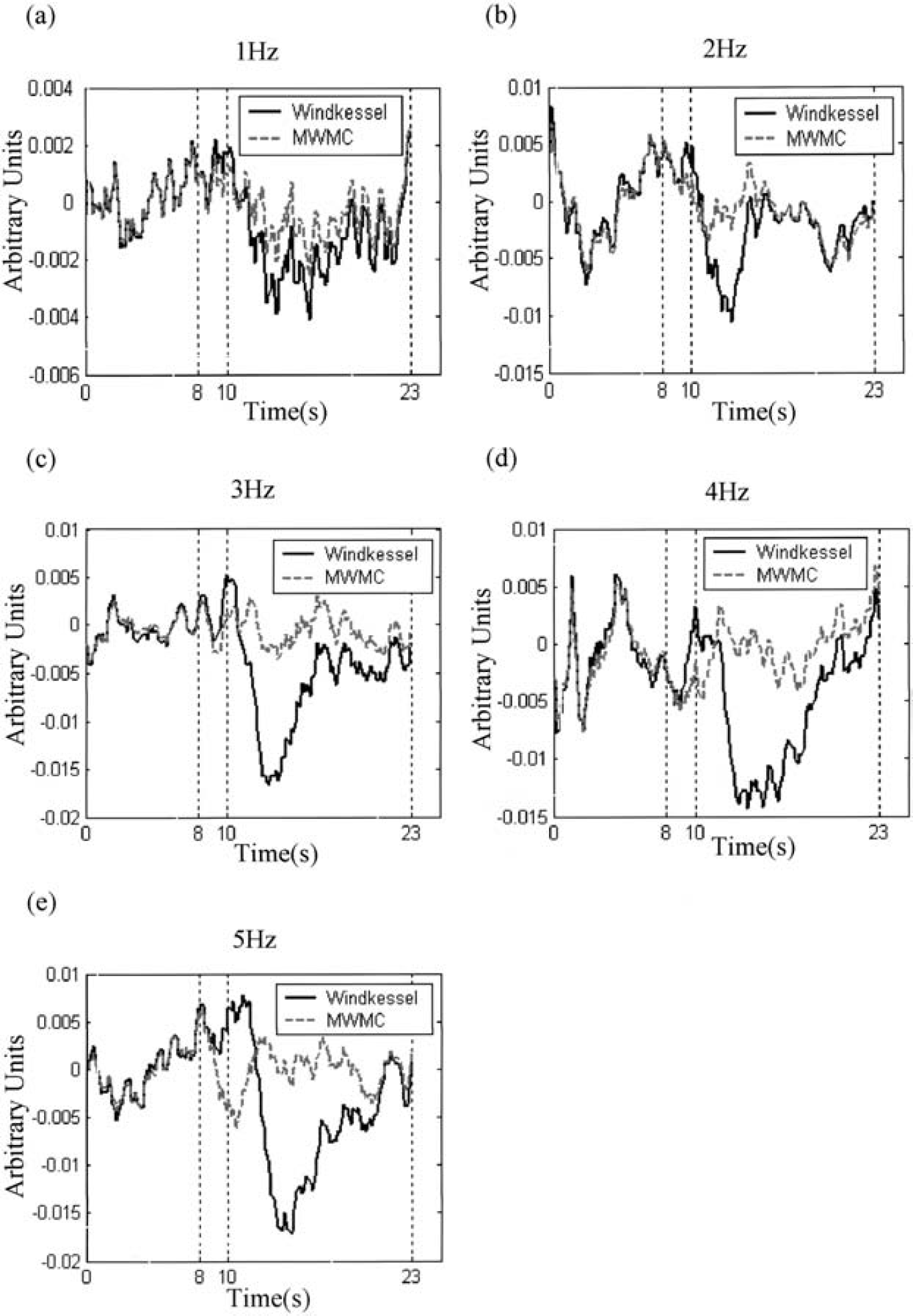
Comparison of model prediction residuals of the Windkessel model and the MWMC for the 1-Hz to 5-Hz data sets. In each figure, the solid line is the prediction residuals from the Windkessel model, and the dashed line is the prediction residuals from the MWMC.

Fig. 10.

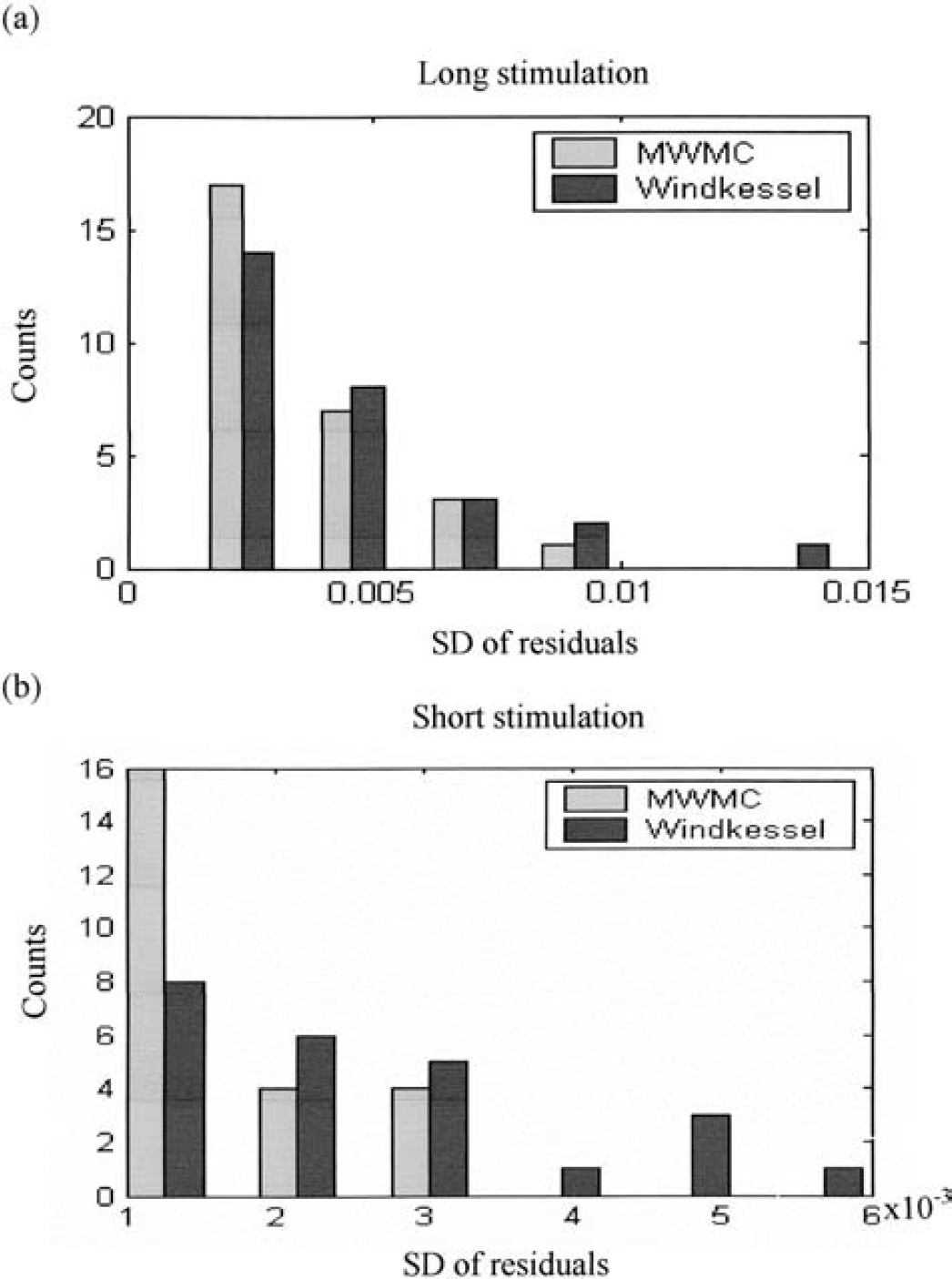
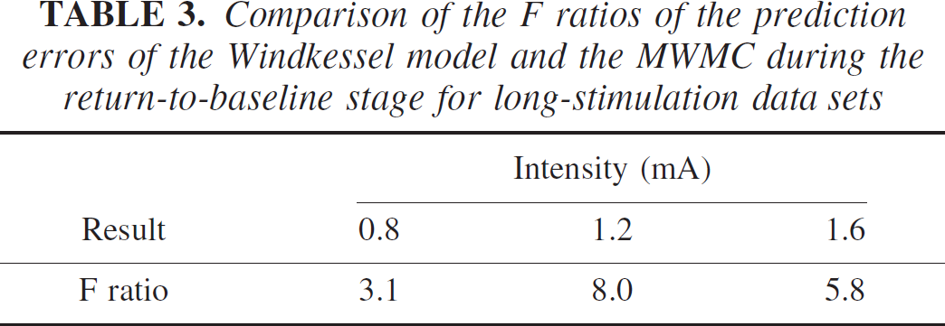
Histograms of the standard deviations of the model prediction residuals from the Windkessel model and the MWMC. (a) Long-stimulation data. (b) Short-stimulation data.

To further compare the performance of the original Windkessel model and the MWMC, we performed the F tests on the model prediction errors for each of the models during the return-to-baseline stage of the mean CBV response over selected animals (149 time points for long stimulus, and 98 data points for short stimulus). The null hypothesis was that the variances of the prediction errors from the two models are not significantly different. The F ratios were calculated with the numerator being the prediction error variance of the Windkessel model, and the denominator being that of the MWMC, shown in Tables 3 and 4. It can be seen that under all stimulus conditions, the calculated F ratio is significant at P < 0.01 (F_0.01 ~ 1.6). This shows that the model prediction errors using the original Windkessel model are significantly larger than those of the MWMC at the 1% level, and that the MWMC can better capture the dynamics of the relationship between normalized changes in CBF and CBV.

Table 3.

Comparison of the F ratios of the prediction errors of the Windkessel model and the MWMC during the return-to-baseline stage for long-stimulation data sets

	Intensity (mA)
Result	0.8	1.2	1.6

F ratio	3.1	8.0	5.8

TABLE 4.

Comparison of the F ratios of the prediction errors of the Windkessel model and the MWMC during the return-to-baseline stage for short-stimulation data sets

	Frequency (Hz)
Result	1	2	3	4	5

F ratio	3.4	6.4	6.8	20.3	36.2

DISCUSSION

This study explored the dynamic relationship between changes in CBF and CBV. Neither the Balloon model (Buxton et al., 1998) nor the original Windkessel model (Maneville et al., 1999) adequately captured the transient relationship between CBF and CBV. A modification of the Windkessel model incorporating compliance as a state variable was presented, and this improved model provided a better fit to the volume changes, particularly during the transient regime of the responses.

The main characteristic of the improved model is the introduction of an additional state variable, c, which captures the delayed compliance in the system. The model was applied to the LDF and OIS measurements under the assumption that blood volume changes occur primarily in the venous compartment, an assumption common to both the original Windkessel and Balloon models. However, the model is not restricted by this assumption. If there are data available supporting the partitioning of the variables to specific compartments of the microvascular structure, the model could be applied to the individual compartments.

Figure 11 shows the time course of the compliance variable c (short stimulation, 5-Hz data as an example), together with the normalized CBF, CBV, and the predicted CBV using the MWMC. It can be seen that the dynamics of c are slower than that of the flow and volume time series. It reaches a maximum approximately 2 seconds after the peaks of flow and volume, and returns to baseline after both flow and volume changes.

Fig. 11.

Comparison of the dynamics of CBF, CBV, the predicted CBV, and the compliance variable c. The 5-Hz data is used as an example.

The differing roles of the two parameters α and τ_c in determining the system dynamics have been discussed earlier. We now turn to the discussion of the role of the parameter β and how it was selected.

Figures 12a and 12b show the mean of the standard deviations of the prediction errors over all animals as β varies for the long- and short-stimulation conditions, respectively. The solid line in each figure is the upper bound of standard deviations of the prediction errors. It can be seen that the minimum prediction error occurs at about β = 0.7 for the long-stimulation condition and at β = 1.6 for the short-stimulation condition. At this stage, we do not understand why β is different for the two different stimulus conditions, and we do not have a theoretical algorithm for calculating the optimal β given the model and the measurement data. These will be the subjects for future investigation.

Fig. 12.

The mean of the standard deviations of the prediction residuals using the MWMC over all animals as β varies. The solid line in each figure is the upper bound of the standard deviations of the prediction errors. (a) Long-stimulation data. (b) Short-stimulation data.

In summary, the relationship between changes in CBF and CBV under different stimulation conditions can be described by a model incorporating delayed compliance with a time constant dependent on stimulus duration.

In all the models evaluated, it was assumed that the blood volume changes occur predominantly in the venous compartment, and that the arteriolar dilation contributed little to the volume changes. These assumptions are not fundamental to the MWMC model, and future work may need to extend this model to different compartments of the microvasculature.

Footnotes

Acknowledgements

The authors thank the reviewers for their constructive comments, which considerably improved the content of this article.

References

Bassingthwaighte

Chaloupka

(1984) Sensitivity functions in the estimation of parameters of cellular exchange. Fed Proc 43:180–184

Buxton

Wong

Frank

(1998) Dynamics of blood flow and oxygenation changes during brain activation: the balloon model. Magn Reson Med 39:855–864

Friston

Mechelli

Turner

Price

(2000) Nonlinear responses in fMRI: the balloon model, volterra kernels and other hemodynamics. Neuroimage 12:466–477

Grubb

Raichle

Eichling

Ter-Pergossian

(1974) The effects of changes in PACO2 on cerebral blood volume, blood flow and vascular mean transit time. Stroke 5:630–639

Jones

Berwick

Johnston

Mayhew

(2001) Concurrent optical imaging spectroscopy and laser-Doppler flowmetry: the relationship between blood flow, oxygenation, and volume in rodent barrel cortex. Neuroimage 13:1002–1015

Jones

Berwick

Mayhew

(2002) Changes in blood flow, oxygenation, and volume following extended stimulation of rodent barrel cortex. Neuroimage 15:474–487

Kleinfeld

Mitra

Helmchen

Denk

(1998) Fluctions and Stimulus-induced changes in blood flow observed in individual capillaries in layers 2 through 4 of rat neocortex. Proc Natl Acad Sci U S A 95:15741–15746

Martindale

Mayhew

Berwick

Jones

Martin

Johnston

Redgrave

Zheng

(2003) The hemodynamic impulse response to a single neural event. J Cereb Blood Flow Metab 23:546–555

Mandeville

Marota

JJA

Kosofsky

Keltner

Weissleder

Rosen

Weisskoff

(1998) Dynamic functional imaging of relative cerebral blood volume during rat forepaw stimulation. Magn Reson Med 39:615–624

10.

Mandeville

Marota

Ayata

Zaharchuk

Moskowitz

Rosen

Weisskoff

(1999) Evidence of a cerebrovascular postarteriole Windkessel with delayed compliance. J Cereb Blood Flow Metab 19:679–689

11.

Mayhew

Zheng

Askew

Hou

Berwick

Coffey

Brown

(1998) An evaluation of linear model analysis techniques for processing images of microcirculation activity. Neuroimage 7:49–71

12.

Nakagawa

Lin

Bereczki

Gesztelyi

Otsuka

Wei

Hans

Acuff

Chen

Pettigrew

Patlak

Blasberg

Fenstermacher

(1995) Blood volumes, hematocrits, and transit-times in parenchymal microvascular systems of the rat brain. In: Diffusion and perfusion magnetic resonance imaging ( Le Bthan

, Ed). New York, NY: Raven Press.

13.

Nilsson

(1984) Signal processor for laser Doppler tissue flowmeters. Med Biol Eng Comput 22:343–348

14.

Roy

Sherrington

(1890) On the regulation of the blood supply of the brain J Physiol (Lond) 11:85–108

15.

Schulte

Wood

Hudetz

(2003) Cortical electrical stimulation alters erythrocyte perfusion pattern in the cerebral capillary network of the rat. Brain Res 963:81–92

16.

Zheng

Martindale

Johnston

Jones

Berwick

Mayhew

(2002) A model of the hemodynamic response and oxygen delivery to brain. Neuroimage 16:617–637

A Model of the Dynamic Relationship between Blood Flow and Volume Changes during Brain Activation

Abstract

Keywords

MATERIALS AND METHODS

Experimental data

Balloon and Windkessel models

Modified Windkessel model with compliance

Sensitivity analysis

RESULTS

DISCUSSION

Footnotes

Acknowledgements

References