Sage Journals: Discover world-class research

Abstract

The graphical analysis uses an ordinary least squares (OLS) fitting of transformed data to determine the total volume of distribution (V_T) and is not dependent upon a compartmental model configuration. This method, however, suffers from a noise-dependent bias. Approaches for reducing this bias include incorporating a presmoothing step, minimizing the squared perpendicular distance to the regression line, and conducting multilinear analysis. The solution proposed by Ogden, likelihood estimation in graphical analysis (LEGA), is an estimation technique in the original (nontransformed) domain based upon standard likelihood theory that incorporates the specific assumptions made on the noise inherent in the measurements. To determine the impact of this new method upon the noise-dependent bias, we compared V_T determinations by compartmental modeling, graphical analysis (GA), and LEGA in 36 regions of interest in dynamic PET data from 25 healthy volunteers injected with [¹¹C]-WAY-100635 and [¹¹C]-McN-5652, which are agents used to image the serotonin 1A receptor and serotonin transporter, respectively. As predicted by simulations, LEGA eliminates the noise-dependent bias associated with GA using OLS. This method is a valuable addition to the tools available for the quantification of radioligand binding data in PET and SPECT.

Keywords

Modeling Kinetic Compartment Logan Serotonin

Several mathematic and conceptual approaches are currently used in the quantification of binding of various radiolabeled ligands to target proteins in the brain using positron emission tomography (PET). One commonly used conceptual framework has been the quantification of the rates of transfer of the radioligand among several compartments (Carson, 1986). Whereas this has been useful for many radioligands, there are exceptions. Graphical analysis (Logan et al., 1990) provides an alternative to quantification of the total volume of distribution (V_T) by ordinary least squares (OLS) fitting of the transformed region of interest time activity curve and the input function. The slope of the transformed data is equivalent to the V_T, and the model assumes no compartmental configuration. Whereas this model allows for rapid determination of V_T, it suffers from a noise-dependent bias that limits its usefulness (Carson, 1993; Slifstein and Laruelle, 2000). Recently, several different approaches to circumventing this limitation have been proposed. These methods include presmoothing the data (Feng et al., 1996, 1993; Logan et al., 2001), estimating parameters by minimizing squared perpendicular distances (Varga and Szabo, 2002), and conducting multilinear analysis (Ichise et al., 2002). Likelihood estimation in graphical analysis (LEGA) differs fundamentally from these in that it gives optimal (in the maximum likelihood sense) estimators of parameters based upon the assumptions of the noise in the data (namely, independent Gaussian noise). The method is based upon a rearrangement of terms in the GA formulation, and estimation is performed using the original, nontransformed data (Ogden, 2003). The fitting is iterative, but the problem can be formulated as a one-dimensional, nonlinear, least squares algorithm. Here we present a comparison of the V_T determinations for the [¹¹C]-WAY-100635 (serotonin 1A antagonist) and [¹¹C]-McN-5652 (serotonin transporter antagonist) compounds using a one-tissue compartment model (1T), two-tissue compartment model (2T), GA, and LEGA in 36 regions of interest (ROI) in 25 healthy volunteers.

MATERIALS AND METHODS

Subjects

Twenty-five healthy volunteers were included in this study. Study criteria for healthy volunteers included the following: (1) aged 18 to 65 years; (2) absence of medical, neurologic, and psychiatric conditions (including alcohol and substance abuse or dependence) based upon a complete structured psychiatric interview with the SCID-NP and SCID II, medical examination and laboratory tests; (3) absence of any medications for at least 2 weeks; (4) absence of exposure to 3,4-methylenedioxymethamphetamine (MDMA, ecstasy); (5) absence of significant medical conditions including a history of head injury with loss of consciousness; and (6) absence of pregnancy. Volunteers with a history of a mood or psychotic disorder in their first-degree relatives were excluded. The Institutional Review Boards of Columbia Presbyterian Medical Center and the New York State Psychiatric Institute approved the protocol. Subjects gave written informed consent after an explanation of the study.

Positron emission tomography protocol

Preparation of tracers and determination of arterial input indices were obtained as previously described for [11C]-McN-5652 (Parsey et al., 2000a) and [¹¹C]-WAY-100635 (Parsey et al., 2000b). After an Allen test and subcutaneous administration of 2% lidocaine, a catheter was inserted in the radial artery. A venous catheter was inserted in a forearm vein on the opposite side. Fiducial markers filled with C-11 (approximately 2 μCi /marker at time of injection) were taped on the subjects head. Head movement was minimized with a polyurethane head immobilizer system (Soule Medical, Tampa, FL, U.S.A.), which was molded around the head of the subject. Positron emission tomography (PET) imaging was performed with the ECAT EXACT HR+ (Siemens/CTI, Knoxville, TN, U.S.A.) (63 slices covering an axial field of view of 15.5 cm, axial sampling of 2.46 mm, 3D mode, and in plane and axial resolution of 4.4 and 4.0 mm full width half-maximum at the center of the field of view, respectively). After injection of [¹¹C]-McN-5652 as an IV bolus over 45 seconds using an injection pump, emission data were collected in 3D mode for 130 minutes as 22 successive frames of increasing duration (3 × 20 seconds, 3 × 1 minute, 3 × 2 minutes, 2 × 5 minutes, 11 × 10 minutes). Images were reconstructed to a 128 × 128 matrix (pixel size of 2.5 × 2.5 mm²) with attenuation correction using a 10-minute transmission scan and a Shepp 0.5 filter (cutoff 0.5 cycles/projection rays). After injection of [¹¹C]-WAY-100635 as an IV bolus over 45 seconds using an injection pump, emission data were collected in 3D mode for 110 minutes as 20 successive frames of increasing duration (3 × 20 seconds, 3 × 1 minute, 3 × 2 minutes, 2 × 5 minutes, 9 × 10 minutes).

Image analysis

Image analysis was performed using MEDX software (Sensor Systems, Inc., Sterling, VA, U.S.A.). Preliminary time activity curves of 20 PET frames were generated to determine whether there was any head motion during the individual frame acquisition. Frames in which motion was detected were aligned and registered to the previous frame or to a mean image using automated image registration (AIR) software (Woods et al., 1992). No attempt was made to correct for transmission-emission mismatch in reconstruction. Regions of interest (ROI) were traced based upon brain atlases (Duvernoy, 1991; Talairach and Tournoux, 1988) and published reports (Kates et al., 1997; Killiany et al., 1997). 17 ROI were drawn on both left and right hemispheres: anterior cingulate cortex (ACIN), amygdala (AMY), cingulate cortex (excluding anterior and posterior cingulate, i.e., body of cingulate; CIN), dorsal caudate (DCA), dorsal putamen (DPU), dorso-lateral prefrontal cortex (DLPFC), entorhinal cortex (ENT), hippocampus (HIP), insular cortex (INS), medial prefrontal cortex (MPFC), occipital cortex (OCC), orbital prefrontal cortex (OPFC), parietal cortex (PC), temporal cortex (TC), thalamus (THA), uncus (UNC), and ventral striatum (VST). The midbrain (MID, used only in [¹¹C]-McN-5652 studies) and cerebellum (CER, used in both studies) were drawn as single-centered ROI. A fixed volume elliptical ROI (2 cm³) was placed on the raphe nuclei (RN), a composite of mostly the dorsal and median raphe nuclei, on a mean [¹¹C]-WAY-100635 PET image for each subject because the boundaries of this structure cannot be identified on MRI. There were a total of 36 ROI for each ligand. MRIs were segmented as previously described (Abi-Dargham et al., 1999), and within cortical regions, only the voxels classified as gray matter were used to measure PET activity distribution.

Magnetic resonance imaging acquisition and segmentation

MRIs were acquired on a GE 1.5 T Signa Advantage system. A sagittal scout (localizer) was performed to identify the AC-PC plane (1 minute). A transaxial T1 weighted sequence with 1.5 mm slice thickness was acquired in a coronal plane orthogonal to the AC-PC plane over the whole brain with the following parameters: 3-dimensional SPGR (Spoiled Gradient Recalled Acquisition in the Steady State); TR 34 msec; TE 5 msec; flip angle of 45 degrees; slice thickness 1.5 mm and zero gap; 124 slices; field of view of 22 × 16 cm; with 256 × 192 matrix, reformatted to 256 × 256, yielding a voxel size of 1.5 mm × 0.9 mm × 0.9 mm; time of acquisition of 11 minutes. MRI segmentation between gray matter (GM), white matter (WM), and CSF pixels was performed as previously described (Abi-Dargham et al., 1999).

Derivation of regional total distribution volumes

Binding was quantified using either a one-tissue compartment kinetic model (1T) for the [¹¹C]-McN-5652 compound (Parsey et al., 2000a), a two-tissue compartment kinetic model (2T) for the [¹¹C]-WAY-100635 compound (Parsey et al., 2000b), graphical analysis of Logan using OLS regression (Logan et al., 1990), or LEGA (Ogden, 2003; Ogden et al., 2002). When using GA, the last eight data points were fit with each ligand. The compartmental model included the arterial plasma compartment (C_a), the intracerebral free and nonspecifically bound compartment (nondisplaceable compartment, C₂), and the specifically bound compartment (C₃). The equilibrium distribution volume of a compartment i (V_i, mL g⁻¹) was defined as the ratio of the tracer concentration in this compartment to the free plasma concentration at equilibrium

V_{i} = \frac{C_{i}}{f_{1} C_{a}}

V₂ and V₃ were defined as the distribution volumes of the second (nondisplaceable) and third (specific) compartments, respectively. V_T was defined as the total regional equilibrium distribution volume, equal to the sum of V₂ and V₃. We assumed the following: (1) that cerebellar V_T represents only free and nonspecific binding and provides a reasonable estimate of V₂ in the ROI and (2) that the contribution of plasma total activity to the regional activity was calculated assuming a 5% blood volume in the ROI and subtracted from the regional activity prior to analysis (Mintun et al., 1984).

Likelihood estimation in graphical analysis

The most popular general-purpose technique for estimation is maximum likelihood. Almost all of the standard statistical methodologies (regression, ANOVA, etc.) have their basis in likelihood theory. When the model for the data is correctly specified, applying likelihood-based methods has many advantages over other approaches (consistency, efficiency, etc.).

The basis for graphical analysis is given by the relationship (Logan et al., 1990):

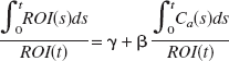
\frac{\int_{0}^{t} R O I (s) d s}{R O I (t)} = γ + β \frac{\int_{0}^{t} C_{a} (s) d s}{R O I (t)}

(1)

for all time points past some “equilibrium” time point. In this expression ROI(t) and C_a(t) are taken to represent the “true” concentration of the ligand in the region and in the plasma, respectively, at time t. The slope parameter β is the total volume of distribution for the region. The intercept parameter γ may be regarded as a nuisance parameter. When blood is sampled during the scan, the plasma concentration is modeled based on data assumed to be independent of PET measurements. For the purposes of estimating β and γ fitted values for the plasma curve are substituted in Equation 1 for each ROI, and the variability in estimating the curve is subsequently neglected.

The standard simple linear regression model is expressed as Y_i = γ + βx_i + ε _i for fixed and known predictors x₁, x₂, …, xn. The error in the model is assumed to be additive, uncorrelated, and homoscedastic and to affect only the “response variables” Y₁, Y₂, …, Y_n. In this case, applying the usual OLS procedure gives maximum likelihood estimators for γ and β that are exactly unbiased. If OLS regression methods are applied when assumptions on the errors do not hold, the estimation properties cannot be expected to hold. If, for instance, the predictor variables (the x_i values) are also measured with additive error (independent of the error on the Y_i values), then the result of applying OLS methods will be a negative bias for the estimator of β (see, e.g., Fuller, 1987). In the application of OLS to the model given in Equation 1, the error is multiplicative for both the x and Y variables (and it is the same in both cases). The result of this, as showed by Slifstein and Laruelle (2000), is an estimator that is negatively biased for β.

The solution proposed by Ogden (2003) is an estimation technique in the original (nontransformed) domain based upon standard likelihood theory that incorporates the specific assumptions made on the noise inherent in the measurements. By writing R_i * = ROI(t_i) (“noise-free” data) and expressing the integral of in terms of the R_i* values, Equation 1 can be rearranged so as to give a recursive relationship for each R_i*

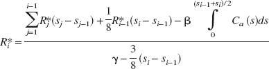
R_{i}^{*} = \frac{\sum_{j = 1}^{i = 1} R_{j}^{*} (s_{j} - s_{j - 1}) + \frac{1}{8} R_{i - 1}^{*} (s_{i} - s_{i - 1}) - β \int_{0}^{{(s_{i - 1} + s_{i})}^{2}} C_{a} (s) d s}{γ - \frac{3}{8} (s_{i} - s_{i - 1})}

for i = k, k + 1, …, n, where s_i represents the endpoint of the ith frame (and the beginning point of frame i + 1). In other words, given the parameters of the Logan relationship, the partial integrals of the plasma curve, and the integrated region activity up to time s_k, the “noise-free” data may be computed exactly.

In practice, all R_i* values are observed with error: R_i = R_i* + ε_i, i = 1, 2, …, n. If the errors are assumed to be independent Gaussians with equal variance, then the maximum likelihood estimator is obtained by minimizing the quantity Σ ⁿ _{i = k} (R_i − R_i*)² over all choices of γ and β. The maximum likelihood estimator of is the value of that minimizes the above sum. Note that this also corresponds to the least-squares estimation of the parameters. If the errors are not assumed to have equal variances, then the sum above may be replaced by a weighted version: Σⁿ_{i = k} w_i (R_i − R_i*)², in which the optimal weights would be inversely proportional to the variances of the R_i values. Minimizing this will result in maximum likelihood estimators.

There is no closed-form expression for the estimators; they must be computed using nonlinear optimization algorithms. To speed up the estimation process, Ogden (2003) showed that for a given value of γ, the estimation of β is linear. Thus the optimization process can be accomplished using a one-dimensional (on γ) optimization routine, which increases the speed of convergence.

For practical application, it is necessary to make a choice of k, the index denoting the time point after which the Logan relationship holds. This is true when using OLS or any of the variants that have been proposed. One option is to use visual inspection of the “Logan plots” to determine an appropriate value of k. Although the LEGA estimation takes place in the original (nontransformed) domain, these plots still provide useful information for determining this index. Alternatively, a number of other methods for choosing k in graphical analysis that are also applicable for LEGA are discussed in Ichise et al. (2002). In the analysis described here, the value of k was chosen based upon visual inspection of many Logan plots for each ligand considered.

RESULTS

McNeil 5652

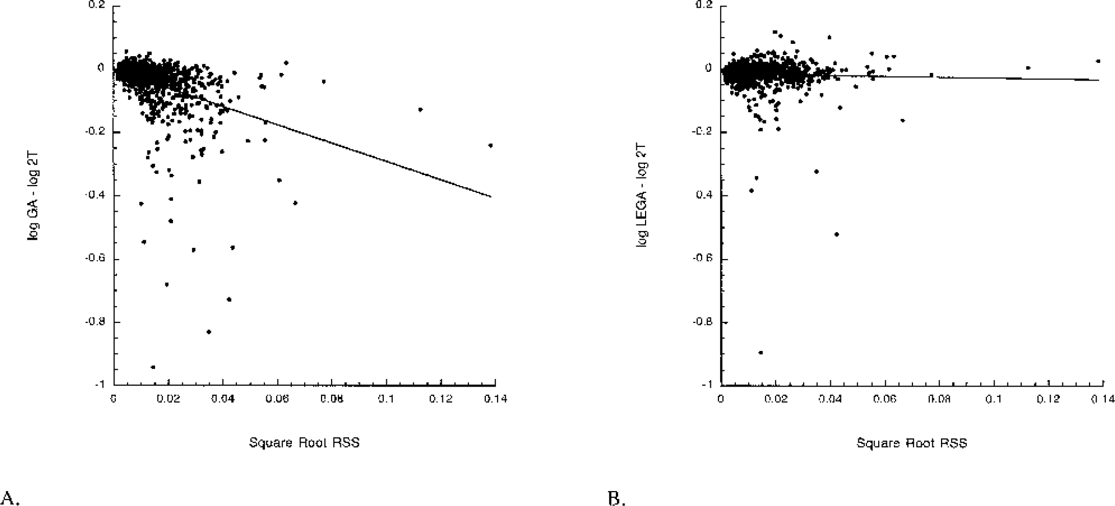
V_T determinations from GA and LEGA are compared with 1T. GA underestimates 1T [¹¹C]-McN-5652 V_T in several regions, most notably the VST, AMY, and DCA (Fig. 1). The LEGA method closely approximates 1T V_T in nearly all regions. Across all 36 regions and all 25 subjects, several regions fall below the line of identity when GA V_T is compared with 1T V_T (Fig. 2A). When V_T determined by LEGA is compared with 1T, however, there is a more even distribution of points above and below the line (Fig. 2B). To demonstrate the noise-dependent bias inherent in GA, the square root of the residual sum of squares of the LEGA fit was plotted against the log of the difference between V_T as determined by GA and V_T from 1T. As the square root of the residual sum of squares increases, the underestimation by GA increases (Fig. 3A). In contrast, there is no bias when using the LEGA method (Fig. 3B).

FIG. 1.

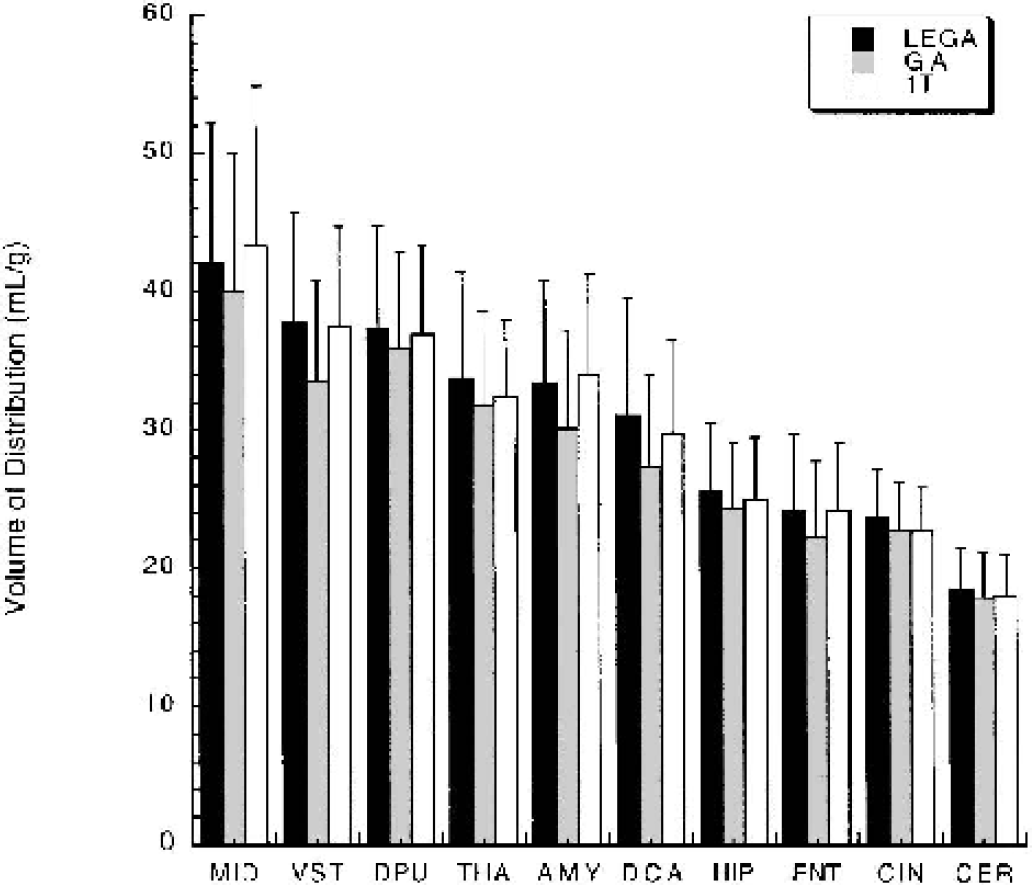
[¹¹C]-McN-5652 V_T determinations by LEGA, GA using OLS, and 1T. For clarity, only several representative left sided regions are displayed. The underestimation of GA compared with 1T is not observed with LEGA. OLS, ordinary least squares; GA, graphical analysis; LEGA, likelihood estimation in GA; 1T, one-tissue compartment kinetic model.

FIG. 2.

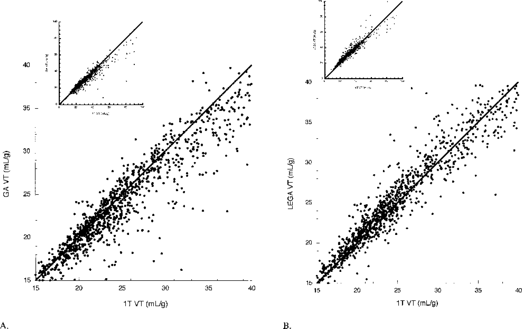
Greater underestimation of [¹¹C]-McN-5652 V_T by GA than LEGA relative to 1T. (A) Correlation between V_T determinations by GA and 1T. (B) V_T determinations by LEGA and 1T. Insets in both panels display the data over all possible points. The main figures display a truncated range for clarity. Solid line in both graphs is the line of identity. GA, graphical analysis; LEGA, likelihood estimation in GA; 1T, one-tissue compartment kinetic model.

FIG. 3.

LEGA does not have the GA noise-dependent bias in [¹¹C]-McN-5652 V_T determinations. (A) Noise-dependent bias in GA vs. 1T: y = −727x + 0.017. (B) Lack of noise-dependent bias in LEGA vs. 1T. y = 0.101x + 0.016. Ordinate in each panel is the square root of the residual sum of squares between the data and the LEGA fit. GA, graphical analysis; LEGA, likelihood estimation in GA; 1T, one-tissue compartment kinetic model.

WAY 100635

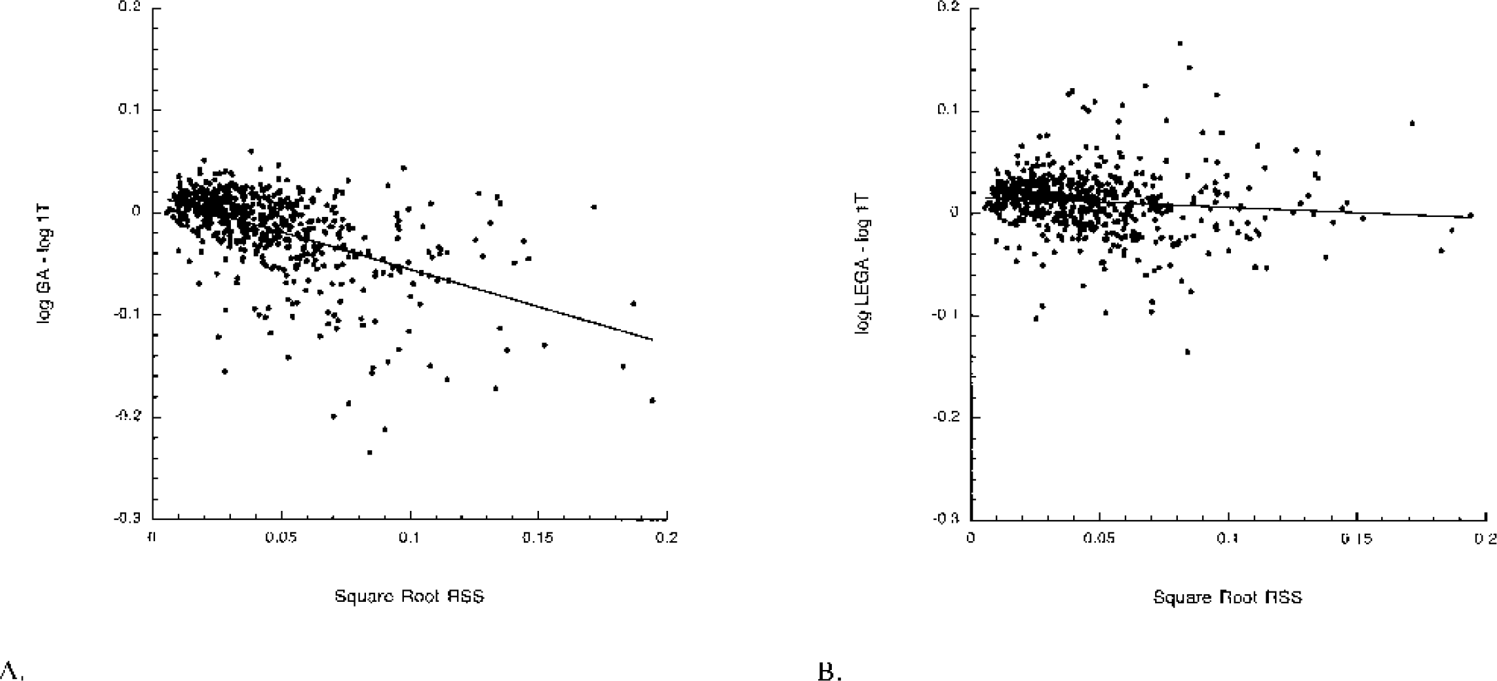
V_T determinations from GA and LEGA are compared with 2T for the [¹¹C]-WAY-100635 compound. GA underestimates 2T in many regions, most notably in the UNC and HIP (Fig. 4). LEGA more closely approximates 2T in most regions. Across all 36 brain regions in 25 subjects, GA underestimates V_T compared with 2T (Fig. 5A). LEGA, in contrast, generates results that are more evenly distributed around the line of identity (Fig. 5B). The underestimation in GA as a function of increasing noise (Fig. 6A) is largely eliminated when LEGA is used (Fig. 6B).

FIG. 4.

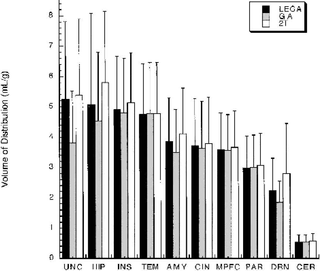
[¹¹C]-WAY-100635 V_T determinations by LEGA, GA with OLS, and 2T. For clarity, several representative left sided regions are displayed. The underestimation of GA compared with 2T is not observed with LEGA. GA, graphical analysis; LEGA, likelihood estimation in GA; OLS, ordinary least squares; 2T, two-tissue compartment kinetic model.

FIG. 5.

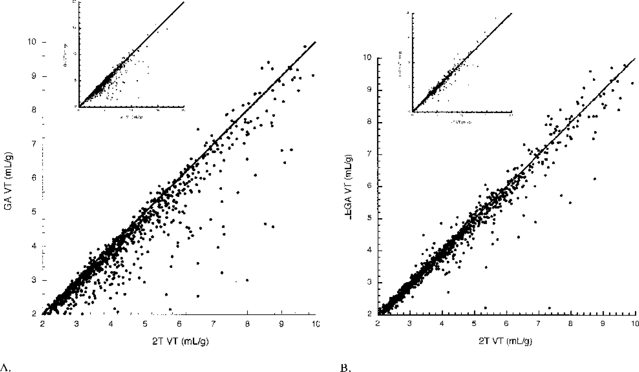
Greater underestimation of [¹¹C]-WAY-100635 V_T by GA than LEGA relative to 2T. (A) Correlation between V_T determinations by GA using OLS and 2T. (B) V_T determinations by LEGA and 2T. Insets in both panels display the data over all possible points. The main figures display a truncated range for clarity. Solid line in both graphs is the line of identity. GA, graphical analysis; LEGA, likelihood estimation in GA; OLS, ordinary least squares; 2T, two-tissue compartment kinetic model.

FIG. 6.

LEGA does not have the GA noise-dependent bias in [¹¹C]-WAY-100635 V_T determinations. (A) Noise-dependent bias in GA vs. 2T: y = −2.90x − 0.002. (B) Lack of noise-dependent bias in LEGA vs. 1T. y = −0.135 − 0.015. Ordinate in each panel is the square root of the residual sum of squares between the data and the LEGA fit. GA, graphical analysis; LEGA, likelihood estimation in GA.

DISCUSSION

The graphical approach to neuroreceptor quantification allows the determination of the total volume of distribution in a robust and rapid manner that is independent of any particular compartmental configuration. The major limitation of this method, however, has been the well-documented noise-dependent bias. The bias is a consequence of the violations of the assumptions necessary for performing ordinary least squares fitting in a simple linear regression model. Specifically, OLS regression is appropriate when the response variables are measured with independent additive noise and the predictor variables are fixed, but in the case of straightforward application to GA, error in the response is multiplicative rather than additive, the predictors are measured with error, and the errors in the predictor are strongly correlated with the errors in the response. As occurs in similar situations of regression assumptions being violated, the result is a negative bias in the estimate of the slope.

The LEGA method is based not upon an adjustment of either the data or the method but rather upon applying very general established (and optimal) estimation techniques specifically to the GA scenario, explicitly taking into account the assumptions made upon the data. By doing so, the new method will not suffer from problems of bias. We previously reported that, in simulations, the LEGA method does in fact eliminate the noise-dependent bias associated with GA. The purpose of this report is to determine to what extent this impacted the quantification of specific neurotransmitter systems with common radioligands. We have demonstrated that the noise-dependent bias of GA with OLS regression exists to differing extents in data from two radiotracers, [¹¹C]-WAY-100635 and [¹¹C]-McN-5652. As predicted by the simulations, the use of LEGA to determine V_T does not suffer from such problems of bias. In simulations, we have seen that this improvement may occur at the expense of greater variance. In the data sets examined in this paper, however, this increase in variance is not apparent. One major implication for this method is that it should provide an alternative to voxel based kinetic modeling approaches. Voxel maps of the total distribution volumes are presented in Fig. 7. Future work will be aimed at characterizing the behavior of LEGA in other radiotracers.

FIG. 7.

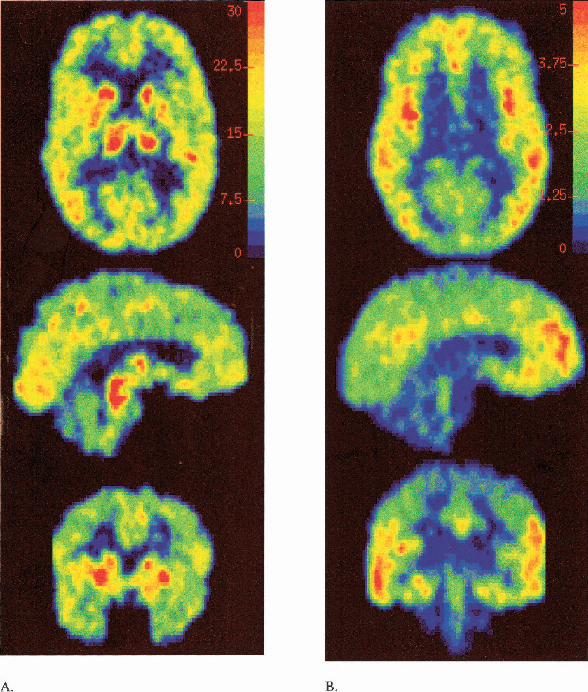
Smoothed voxel maps of a [¹¹C]-McN-5652 V_T (B) and [¹¹C]-WAY-100635 V_T (A). Transaxial, sagittal, and coronal views from top to bottom. The top panel contains the calibration bar.

Footnotes

Acknowledgment:

The authors thank the employees to the Brain Imaging Division and Clinical Evaluation Core of the Conte Center for the Neurobiology of Major Depression, the Kreitchman PET Center, and the Radiopharmaceutical Lab for all of their expert help and support.

References

Abi-Dargham

Simpson

Kegeles

Parsey

Hwang

Anjilvel

Zea-Ponce

Lombardo

Van Heertum

Mann

Foged

Halldin

Laruelle

(1999) PET studies of binding competition between endogenous dopamine and the D1 radiotracer [11C]NNC 756. Synapse 32:93–109

Carson

(1986) Parameter estimation in positron emission tomography. In: Positron emission tomography and autoradiography: principles and applications for the brain and heart), New York: Raven Press, pp. 347–390

Carson

(1993) PET parameter estimation using linear integration methods: bias and variability consideration. In: Quantification of brain function: tracer kinetics and image analysis in brain PET: proceedings of Brain PET '93 Akita: Quantification of Brain Function, Akita, Japan, 29–31 May, 1993, New York: Excerpta Medica, pp. 499–507

Duvernoy

(1991) The human brain. Surface, three-dimensional sectional anatomy and MRI. New York: Springer-Verlag Wien

Feng

Huang

Wang

(1996) An unbiased parametric imaging algorithm for nonuniformly sampled biomedical system parameter estimation. IEEE Trans Med Imaging 15:512–518

Feng

Wang

Huang

(1993) A study on statistically reliable and computationally efficient algorithms for generating local cerebral blood flow parametric images with positron emission tomography. IEEE Trans Med Imaging 12:182–188

Fuller

(1987) Measurement error models. New York: Wiley

Ichise

Toyama

Innis

Carson

(2002) Strategies to improve neuroreceptor parameter estimation by linear regression analysis. J Cereb Blood Flow Metab 22:1271–1281

Kates

Abrams

Kaufmann

Breiter

Reiss

(1997) Reliability and validity of MRI measurement of the amygdala and hippocampus in children with fragile X syndrome. Psychiat Res Neuroimag 75:31–48

10.

Killiany

Moss

Nicholson

Jolesz

Sandor

(1997) An interactive procedure for extracting features of the brain from magnetic resonance images: The lobes. Hum Brain Mapp 5:355–363

11.

Logan

Fowler

Volkow

Ding

Wang

Alexoff

(2001) A strategy for removing the bias in the graphical analysis method. J Cereb Blood Flow Metab 21:307–320

12.

Logan

Fowler

Volkow

Wolf

Dewey

Schlyer

MacGregor

Hitzemann

Bendriem

Gatley

(1990) Graphical analysis of reversible radioligand binding from time-activity measurements applied to [N-11C-methyl]-(−)-cocaine PET studies in human subjects. J Cereb Blood Flow Metab 10:740–747

13.

Mintun

Raichle

Kilbourn

Wooten

Welch

(1984) A quantitative model for the in vivo assessment of drug binding sites with positron emission tomography. Ann Neurol 15:217–227

14.

Ogden

(2003) On estimation of kinetic parameters in graphical analysis of PET imaging data. Statistics in Medicine (In press)

15.

Ogden

Parsey

Mann

(2002) Likelihood approach to parameter estimation in Logan graphical analaysis. Neuroimage 16:S73

16.

Parsey

Kegeles

Hwang

Simpson

Abi-Dargham

Mawlawi

Slifstein

Van Heertum

Mann

Laruelle

(2000a) In vivo quantification of brain serotonin transporters in humans using [11C]McN 5652. J Nucl Med 41:1465–1477

17.

Parsey

Slifstein

Hwang

Abi-Dargham

Simpson

Mawlawi

Guo

Van Heertum

Mann

Laruelle

(2000b) Validation and reproducibility of measurement of 5-HT1A receptor parameters with [carbonyl-11C]WAY-100635 in humans: comparison of arterial and reference tissue input functions. J Cereb Blood Flow Metab 20:1111–1133

18.

Slifstein

Laruelle

(2000) Effects of statistical noise on graphic analysis of PET neuroreceptor studies. J Nucl Med 2083–2088

19.

Talairach

Tournoux

(1988) Co-planar stereotactic atlas of the human brain. Three-dimensional proportional system: an approach of cerebral imaging. New York: Theime Medical Publisher

20.

Varga

Szabo

(2002) Modified regression model for the Logan plot. J Cereb Blood Flow Metab 22:240–244

21.

Woods

Cherry

Mazziotta

(1992) Rapid automated algorithm for aligning and reslicing PET images. J Comput Assist Tomogr 16:620–633

Determination of Volume of Distribution using Likelihood Estimation in Graphical Analysis: Elimination of Estimation Bias

Abstract

Keywords

MATERIALS AND METHODS

Subjects

Positron emission tomography protocol

Image analysis

Magnetic resonance imaging acquisition and segmentation

Derivation of regional total distribution volumes

Likelihood estimation in graphical analysis

RESULTS

McNeil 5652

WAY 100635

DISCUSSION

Footnotes

Acknowledgment:

References