Oscillations in Cerebral Blood Flow Detected with a Transcranial Doppler Index

Abstract

Although transcranial Doppler ultrasound (TCD) has been used to detect oscillations in CBF, interpretation is severely limited, since only blood velocity and not flow is measured. Oscillations in vessel diameter could, therefore, mask or alter the detection of those in flow by TCD velocities. In this report, the authors use a TCD-derived index of flow to detect and quantify oscillations of CBF in humans at rest. A flow index (FI) was calculated from TCD spectra by averaging the intensity weighted mean in a beat-by-beat manner over 10 seconds. Both FI and TCD velocity were measured in 16 studies of eight normal subjects at rest every 10 seconds for 20 minutes. End tidal CO₂ and blood pressure were obtained simultaneously in six of these studies. The TCD probe position was meticulously held constant. An index of vessel area was calculated by dividing FI by velocity. Spectral estimations were obtained using the Welch method. Spectral peaks were defined as peaks greater than 2 dB above background. The frequencies and magnitudes of spectral peaks of FI, velocity, blood pressure, and CO₂ were compared with t tests. The Kolmogorov-Smirnov test was used to further confirm that the data were not white noise. In most cases, three spectral peaks (a, b, c) could be identified, corresponding to periods of 208 ± 93, 59 ± 31, and 28 ± 4 (SD) seconds for FI, and 196 ± 83, 57 ± 20, and 28 ± 6, (SD) seconds for velocity. The magnitudes of the spectral peaks for FI were significantly greater (P < 0.02) than those for velocity. These magnitudes corresponded to variations of at least 15.6%, 9.8%, and 6.8% for FI, and 4.8%, 4.2%, and 2.8% for velocity. The frequencies of the spectral peaks of CO₂ were similar to those of FI with periods of 213 ± 100, 60 ± 46, and 28 ± 3.6 (SD) seconds. However, the CO₂ spectral peak magnitudes were small, with an estimated maximal effect on CBF of (±) 2.5 ± 0.98, 1.5 ± 0.54, and 1.1 ± 0.31 (SD) percent. The frequencies of the blood pressure spectral peaks also were similar, with periods of 173 ± 81, 44 ± 8, and 26 ± 2.5 (SD) seconds. Their magnitudes were small, corresponding to variations in blood pressure of (±) 2.1 ± 0.55, 0.97 ± 0.25, and 0.72 ± 0.19 (SD) percent. Furthermore, coherence analysis showed no correlation between CO₂ and FI, and only weak correlations at isolated frequencies between CO₂ and velocity, blood pressure and velocity, or blood pressure and FI. The Kolmogorov-Smirnov test distinguished our data from white noise in most cases. Oscillations in vessel flow occur with significant magnitude at three distinct frequencies in normal subjects at rest and can be detected with a TCD-derived index. The presence of oscillations in blood velocity at similar frequencies but at lower magnitudes suggests that the vessel diameters oscillate in synchrony with flow. Observed variations in CO₂ and blood pressure do not explain the flow oscillations. Ordinary TCD velocities severely underestimate these oscillations and so are not appropriate when small changes in flow are to be measured.

Regular oscillations of CBF have been reported in both animal models and human studies with periods of oscillations ranging from 5 to 120 seconds and with amplitudes of 14% to 40% of baseline values (Fasano et al., 1988; Friberg and Olsen, 1991; Rosenblum et al., 1987; Meyerson et al., 1991; Hudetz et al., 1992). Transcranial Doppler ultrasound (TCD) also has been used to detect oscillations in blood velocity in both normal subjects and patients by several authors (Diehl et al., 1996; Droste et al., 1994; Newell et al., 1996; Steinmeier et al., 1996). The TCD studies are controversial, however, since on one hand they are noninvasive and convenient, whereas on the other hand, their interpretation is limited because only velocity and not flow is measured directly. If changes in flow could be reliably derived from TCD signals, the superior time resolution and portability of this modality would offer advantages over invasive methods (Sioutos et al., 1995) or those with slower time responses (Friberg and Olsen, 1991).

We have previously described an index, FI, derived from the entire TCD spectrum, which is proportional to flow through the insonated vessel, providing quantitative measurement of flow trends (Hatab et al., 1997; Giller et al., 1997; Giller et al., 1998). In this report, we use this index to detect oscillations in signals obtained from human subjects at rest.

METHODS

Subjects

Subjects were volunteers without known cerebrovascular disease. Sixteen recordings from eight subjects were obtained. Two subjects had two studies, one subject had three studies, and one subject had five studies. All studies were performed on different days.

Data acquisition and protocols

The TCD signals were obtained with a commercially available device (Pioneer 2020, Nicolet, Madison, WI, U.S.A.) using a 2-MHz ultrasound probe and a headband provided by the manufacturer or one that was custom-made for the subject (Giller et al., 1996) to hold the probe in constant position. The middle cerebral artery (MCA) was insonated in all cases according to known criteria (Aaslid et al., 1982). Equipment availability allowed six recordings to include end tidal CO₂ simultaneously obtained (Nellcor, Model N-1000, Hayward, CA, U.S.A.) with noninvasive measurements of blood pressure (BP) (Ohmeda 2300 Finapres, Louisville, CO, U.S.A.). After placement of probes and transducers, each subject was kept at rest for 10 to 20 minutes before data acquisition. The head was supported and monitored meticulously to ensure absence of even small movements. A movie of bland content was shown to the subject to prevent sleep and lessen the effects of cerebral activation. Movies of active content were earlier found to produce significant variations in the TCD signals.

The CO₂ and BP were recorded continuously for 20 minutes and averages computed for each 10-second interval. The TCD spectra occurring during these same 10-second intervals were saved for off-line computation. A duration of 10 seconds was chosen after trial studies to reduce the amount of variation in the calculated indices.

Data analysis

Calculation of indices. The FI and an area index (AI) (see later) were calculated for each 10-second TCD spectral segment. Details of this calculation have been previously described (Hatab et al., 1997; Giller et al., 1997; Giller et al., 1998). Briefly, the individual spectral waveforms during each of the 10-second intervals were added (pixel to pixel) together to suppress noise and to obtain a single spectrum. At each instant in time, the volume of blood in the ultrasound sample volume flowing at a particular velocity is proportional to the intensity of the TCD signal, coded by the color of the pixel at that time and velocity. The amount of blood flow arising from blood at a particular velocity is, therefore, the product of that velocity with the corresponding intensity. Summing over all velocities yields an index, FI, proportional to flow. Other authors have used this intensity-weighted mean without averaging (Aaslid, 1987; Muller and Casty, 1987; Schregal et al., 1994).

The averaging process used to calculate FI can be viewed as a moving average of the instantaneous FI signal (with a lag of 10 seconds) followed by a decimation. The effects of these maneuvers on the spectral content of the resulting FI time series were explicitly calculated.

Since flow through a vessel is equal to the product of the cross-sectional area of the vessel with the (spatial) mean velocity through the vessel, and since for laminar flow the spatial and time mean velocity are proportional (Nichols and O'Rourke, 1990), we have defined an AI as the FI divided by the ordinary (time mean) TCD velocity. This differs from the usual definition of an AI as the spectral power (sum of ultrasound intensities) and will produce inaccurate trends in area if the proportionality between the spatial mean and time mean of velocity changes during data acquisition.

Computation of power spectra

Averaging every 10 seconds for 20 minutes produced 120 data points, which were considered as a time series with a sampling rate of 0.1 Hz. The data were normalized to its mean, the mean subtracted, and trends noted and removed by subtracting the line of least regression. This produced a data sequence representing percentage changes from the mean for which linear trends have been removed. Since proportionality constants between flow and FI are different for each study, this procedure is necessary for meaningful comparisons.

To determine whether regular oscillations were present in these processed signals, the power spectra were calculated with the Welch algorithm (Hayes, 1996; Bendat and Piersol, 1971) using commercially available software (MATLAB, Mathworks, Natick, MA, U.S.A.). With this method, the data were divided into smaller overlapping segments, the fast Fourier transform (FFT) of each segment calculated, and an average obtained. The result is an estimate of the amount of oscillatory variation in the original signal at each particular frequency. If the data are divided into a greater number of segments, the statistical reliability of the power spectrum estimate rises. The importance of this is underlined by the fact that the FFT of the entire data set (one segment) often is so variable that interpretation is meaningless. However, a larger number of data segments restricts the segment length and so limits the frequency range that can be analyzed. Although the common practice of allowing the segments to overlap by 50% mitigates this problem somewhat, the tradeoff between statistical reliability and band width is inevitable (Hayes, 1996). To analyze variations with periods between 20 and 300 seconds, we used segments of length 30 (corresponding to 300 seconds) overlapped by 50%, which usually resulted in seven segments. In some cases, we used a segment length of 40 when it appeared that lower frequencies might be present (Challis and Kitney, 1991).

This analysis was performed for FI, AI, ordinary TCD velocity, BP, and end tidal CO₂ when available.

Analysis of power spectra

The power spectra were examined for the appearance of peaks defined arbitrarily as elevations of more than 2 dB from the background (spectral value on either side). The frequency (and period) at which peaks appeared and the magnitude of each peak was measured.

The presence of a spectral peak can be interpreted as the presence of oscillation at the corresponding frequency in the original time series. The amplitude of a sine wave that would produce peaks of the same magnitude as those observed was calculated to estimate the amount of variation in the data represented by the spectral peak. The amplitude of this sine wave is referred to as the equivalent sine wave amplitude (ESWA).

The ESWA of the end tidal CO₂ data were converted to millimeters of mercury by multiplying by the mean CO₂, and an estimate of an upper limit of the percentage change induced in CBF was calculated by assuming a 5% change in CBF for every 1-mm Hg change in end tidal CO₂ (Bishop et al., 1986). We chose the upper limit of CO₂ reactivity to be most conservative about discounting the effect of CO₂ on flow.

The magnitudes and periods of the spectral peaks for FI and velocity were averaged and compared with both one- and two-tailed t test.

Coherence

Coherence spectra were calculated between each of the variables FI, velocity, AI, BP, and CO₂ (Bendat and Piersol, 1971; Giller and Iacopino, 1997). A coherence of 1.0 indicates perfect correlation, whereas a coherence of 0.0 suggests little correlation.

Kolmogorov-Smirnov test

To further distinguish our data from white noise, the Kolmogorov-Smirnov test was applied (Masters, 1995). In this test, the hypothesis that the time series in question is white noise may be rejected if the maximum value of the normalized cumulative sum of the FFT of the series exceeds a critical value.

RESULTS

Trends

The FI recordings were examined for trends or slow oscillations (periods greater than 7 minutes). Decreasing trends were seen in four studies, an increasing trend in one study, and slow oscillations in five studies.

Spectral peaks

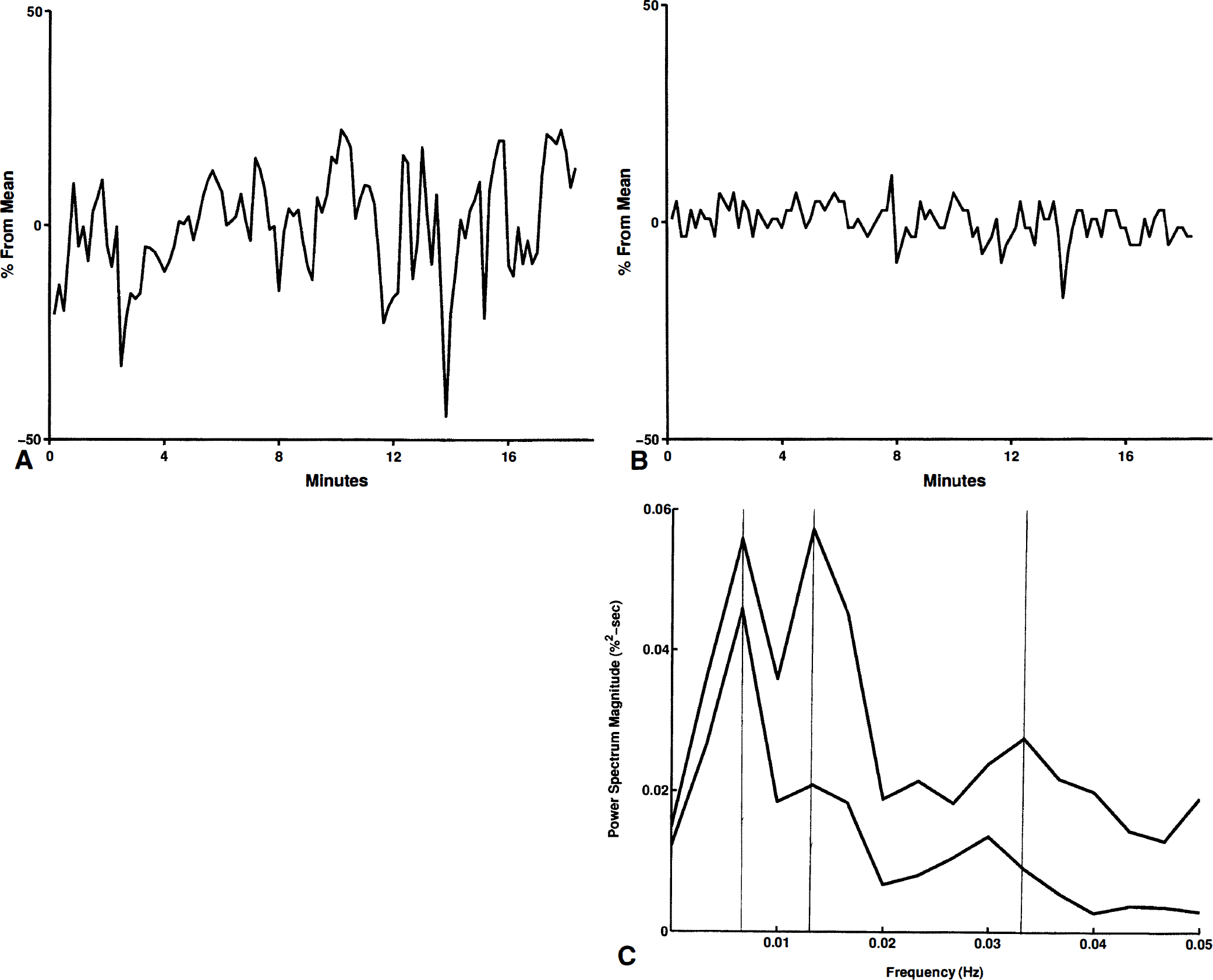
The spectra generally showed three distinct peaks, which we call a, b, and c (Figs. 1 and 2). If only two peaks were present, we considered them as a- and b-peaks if the frequency of the a peak was 0.01 Hz or less, and as b- and c-peaks otherwise. If a peak was not present, it was not included in the denominator of our averages. For example, the mean period of the a-peaks refers to the average period of the peaks in studies showing an a-peak. This strategy allowed comparison of studies showing three peaks in overlapping ranges.

FIG. 1.

(A) Flow index from normal subject averaged every 10 seconds for 20 minutes. (B) Welch spectrum of (A) using windows of 300 seconds with 50% overlap. Notice the presence of three peaks. (C) Same signal as (A) with oscillations corresponding to large peak appearing in (B) filtered out. Oscillations corresponding to the smaller peaks seen in (B) are now apparent (sixth order Chebyshev type I filter). Use of the Kolmogorov-Smirnov test allowed rejection of the hypothesis that this signal represents white noise (P < 0.01).

FIG. 2.

(A) Flow index from normal subject averaged every 10 seconds for 20 minutes. (B) Velocity from same subject and study as (A), at same scale. Notice the smaller variation. (C) Welsh spectra of (A) and (B). The lower curve is 18 × velocity; the upper curve is flow index. The amplitudes of the flow index peaks are far greater than those of velocity, but the frequencies are almost identical.

Two of the FI recordings did not have c-peaks; two of the velocity recordings did not have a-peaks; three of the AI recordings did not have c-peaks; one of the BP recordings did not have a c-peak; all of the CO₂ recordings had three peaks. The remainder of the recordings had three identifiable peaks. A peak extended over a range of frequencies in two a-peaks of FI, two a-peaks of velocity, one a-peak of AI, and an a- and c-peak of BP; the average frequency and period were used in these cases.

The peaks also were grouped in a separate analysis by identifying peaks with frequencies between 0 and 0.013 Hz as a-peaks, between 0.013 and 0.03 Hz as b-peaks, and greater than or equal to 0.03 Hz as c-peaks. The relation between periods, frequencies, and magnitudes of the FI, velocity, BP, and CO₂ was unaltered.

Generally, peaks were found in the power spectra of FI, AI, and velocity at frequencies with corresponding periods of 200, 60, and 30 seconds (Table 1). The mean frequencies of a-, b-, and c-peaks of FI almost exactly match those of velocity (Fig. 2). However, the amplitudes of the FI peaks were significantly greater than those of velocity (Figs. 2 through 4). The ESWA for velocity was less than 3%, indicating almost imperceptible variations in the velocity signal. On the other hand, ESWA for the FI peaks were 7.8%, 4.9%, and 3.4%, respectively, suggesting a variation of at least twice this in the original flow (Fig. 5).

TABLE 1.

Oscillation parameters

		FI	Velocity	AI	Blood pressure	End tidal CO2
Frequency (Hz)	a	.0064 ± .0035	.0069 ± .003	.005 ± .003	.0065 ± .0022	.006 ± .0038
	b	.02 ± .008	.02 ± .007	.023 ± .007	.023 ± .0045	.022 ± .0088
	c	.037 ± .006	.037 ± .007	.037 ± .005	.04 ± .0041	.037 ± .0049
Period (seconds)	a	208 ± 93	196 ± 83	230 ± 81	173 ± 81	213 ± 100
	b	59 ± 31	57 ± 20	51 ± 12	44 ± 8	60 ± 46
	c	28 ± 4	28 ± 6	27 ± 4	26 ± 2.5	28 ± 3.6
Magnitude	a	.039 ± .04	.0034 ± .0033	.037 ± .037	.0024 ± .0012	.0012 ± .00093
	b	.017 ± .021	.0023 ± .001	.012 ± .015	.0051 ± .00023	.00041 ± .0003
	c	.007 ± .006	.001 ± .0005	.004 ± .005	.00029 ± .00014	.0002 ± .00014
ESWA∗(%)	a	7.8	2.4	7.7	2.1 ± .55	2.5 ± .98
	b	4.9	2.1	4.1	.97 ± .25	1.5 ± .54
	c	3.4	1.4	2.6	.72 ± .19	1.1 ± .31

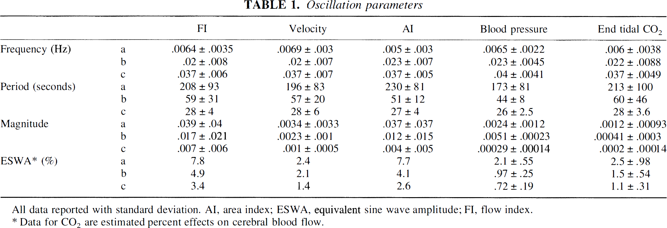
All data reported with standard deviation. AI, area index; ESWA, equivalent sine wave amplitude; FI, flow index.

∗

Data for CO₂ are estimated percent effects on cerebral blood flow.

FIG. 3.

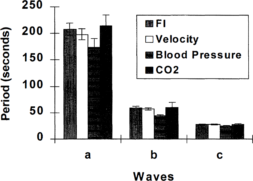
Periods of the three spectral peaks-a, b, and c-of FI, velocity, blood pressure, and end tidal CO₂ averaged over the entire group. Notice almost identical periods. (Standard error [SE] is shown for each bar.)

FIG. 4.

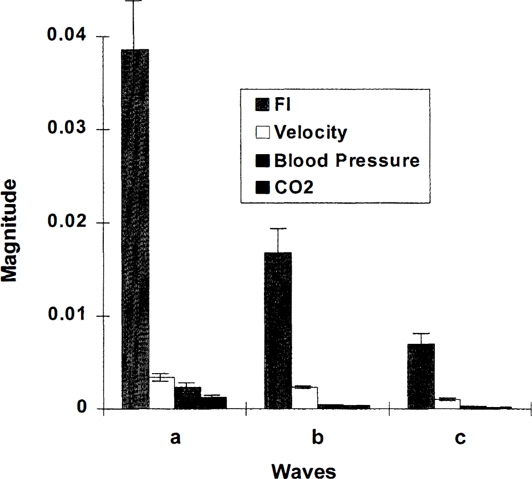
Magnitude of the three spectral peaks-a, b, and c-of FI, velocity, blood pressure, and end tidal CO₂ averaged over entire group. Notice much larger magnitude of FI peaks. (SE is not shown for small bars. See text for values.)

FIG. 5.

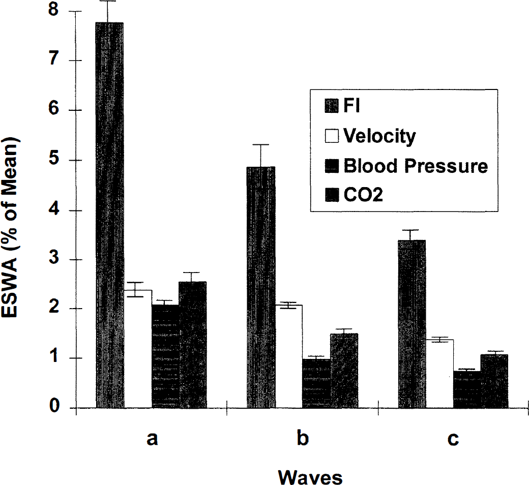
Equivalent sine wave amplitude (ESWA) of FI, velocity, blood pressure, and end tidal CO₂. Peak-to-trough variations are twice the ESWA. (SE is shown.)

Blood pressure and end tidal carbon dioxide

Periods of the spectral peaks of the end tidal CO₂ tracings were 213 ± 100, 60 ± 46, and 28 ± 3.6 (SD) seconds and were almost identical to those of velocity. The estimated maximal changes in CBF were either an increase or decrease by 2.5 ± 0.98, 1.5 ± 0.54, and 1.1 ± 0.31. These were significantly different from the ESWA of FI indicating that the oscillations of FI did not solely arise from variations in end tidal CO₂.

Periods of the BP peaks were 173 ± 81, 44 ± 8, and 26 ± 2.5 (SD) seconds. Their magnitude was significantly smaller than the corresponding peaks belonging to FI, indicating that the oscillations of FI did not solely arise from variations in BP (Figs. 3 and 4).

Coherence

Coherence spectra were calculated between each pair of the variables FI, velocity, AI, BP, and end tidal CO₂. Only isolated peaks in the coherence spectra were seen, except for relatively wide bands of high coherence (above 0.80) between FI and AI, and some bands of coherence (above 0.60) between FI and velocity.

Kolmogorov-Smirnov test

Each recording of FI, velocity, AI, BP, and CO₂ could be distinguished from white noise by the Kolmogorov-Smirnov test, except for one instance of velocity and one instance of BP at the 0.05 level, and two further instances of velocity at the 0.01 level.

DISCUSSION

Although oscillations in CBF have been described in both humans and animals by many investigators (Hudetz et al., 1992; Meyerson et al., 1991; Friberg and Olsen, 1991; Rosenblum et al., 1987; Fasano et al., 1988), the origin of this rhythmicity is unclear. Possible theories include effects of BP, CO₂, autonomic tone, central pacemakers, and entrainment of local flow changes. In this report, we confirm the existence of CBF oscillations in humans, characterize their frequencies using spectral analysis, and indicate their relation to oscillations of vascular diameter.

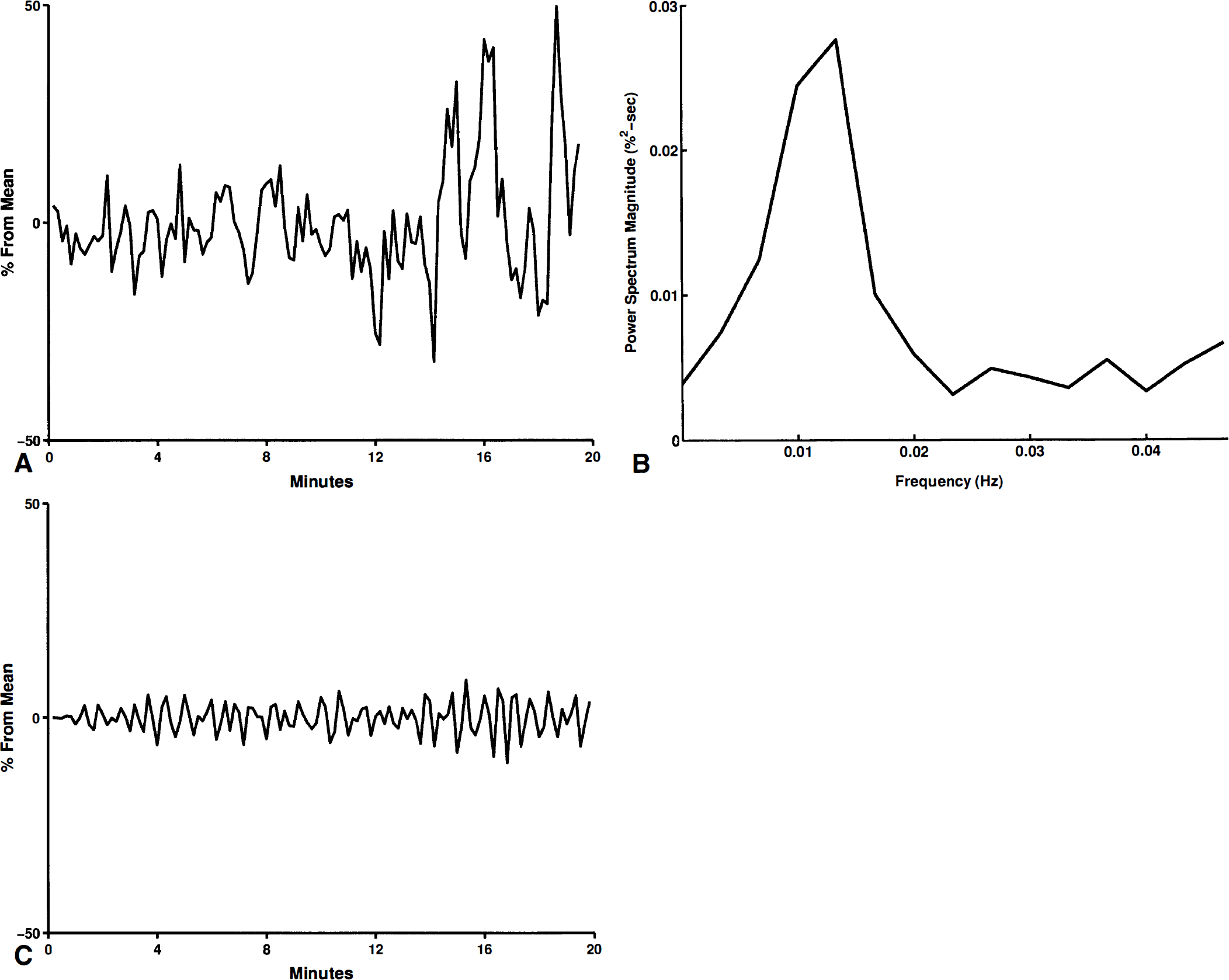
The appearance of three definite peaks (a, b, c) in the FI spectrum confirmed oscillations of FI occurring at the corresponding three frequencies with approximate periods of oscillation of 200, 60 and 30 seconds. The magnitude of the oscillations (7.8%, 4.9%, 3.4%) estimated by ESWA was surprisingly large (Figs. 1 and 2). Notice that an ESWA of 7.8 describes the amplitude of a sine wave with a similar spectrum, so that the peak-to-trough variation of FI is twice this (15.6%). These results establish the resting behavior of FI and suggest the presence of striking synchrony in vasomotion of the cerebral vascular bed, since asynchronous changes would not produce such clear oscillations.

Synchronous vasomotion

To discuss the associated vessel diameter changes, we define a change in vessel diameter occurring at the site of insonation as “in loco,” and a change in diameter occurring away from the site of insonation (either proximal or distal) is referred to as “ex loco.” These are convenient terms, since in loco changes generally alter Doppler velocity but do not change CBF if they are small (Fujii et al., 1991), whereas ex loco changes alter flow and velocity by the same factor.

If there were no in loco changes during the observed oscillations (i.e., if the diameter of the site of insonation was constant), the vessel flow, FI, and velocity all would oscillate at the same magnitude. Since the magnitude of the velocity oscillations was observed to be significantly less than those of FI, the in loco changes must occur in a manner to cancel the variations in velocity. In other words, the in loco diameter increases as flow increases and decreases as flow decreases. Furthermore, an ex loco increase tends to increase flow (and velocity) and so must be accompanied by an in loco increase, which decreases velocity and therefore minimizes any velocity changes. These considerations suggest that the entire cerebrovascular tree must oscillate synchronously. Small differences in ex loco and in loco changes would explain the occurrence of peaks in the velocity spectra.

Our conclusions are in agreement with several prior studies. Simultaneous measurement of basilar artery diameter and brain stem flow in cats has shown oscillations of diameter and flow that are synchronous and in phase (Fujii et al., 1991; Fujii et al., 1990). The reported magnitude of flow variation of ±7.5% would produce a velocity variation of ±13%, again in agreement with our data and prior estimates (Newell et al., 1992; Giller et al., 1993; Droste et al., 1994; Diehl et al., 1996; Steinmeier et al., 1996). This same study showed that changes in vessel diameter alone would not produce flow oscillations because topical application of serotonin selectively constricted the vessel diameter but left flow unaltered. Therefore, in loco as well as ex loco oscillation must have been present. In this animal model, the calculated velocity oscillated with a magnitude greater than that of flow and oscillated out of phase with flow and diameter. This suggests that although flow varies directly with a phasic synchronous diameter change, the magnitude of the flow change may depend on such such factors as the resistance of the microvascular bed to produce velocity changes of various magnitudes.

These conclusions are in agreement with a study comparing velocity oscillations with those of intracranial pressure in humans (Newell et al., 1992) in which velocity was found to vary synchronously and in phase with intracranial pressure. Oscillations of distal (ex loco) vessels must, therefore, be present, since oscillation of MCA diameter alone would produce a velocity signal out of phase with the (flow-induced) cycles of intracranial pressure. Therefore, as in the previous study, the existence of in loco and ex loco diameter changes can be inferred, which is in agreement with our data.

Effects of blood pressure and carbon dioxide

The estimated magnitudes of oscillations in BP were significantly less than those of FI, indicating that the observed FI oscillations did not arise from changes in BP. Our data suggest that the FI variations arise from synchronous phasic changes in vascular diameter, but the origin of this synchrony is unclear. Although possibilities include a “central pacemaker,” we speculate that vasomotion of vascular segments of the cerebral tree may entrain themselves much as other populations of biological oscillations are known to do.

The estimated flow changes arising from oscillations in end tidal CO₂ also were significantly less than those of FI, suggesting that FI oscillations did not arise solely from changes in CO₂. Furthermore, if changes in CO₂ had produced changes in CBF and FI, then proportional changes would have been produced in velocity (Bishop et al., 1986), contrary to our observations. Our assumption that the reactivity of FI is similar to that of velocity (and CBF) is justified by the finding that FI and velocity are tightly correlated (with a slope of 1.008) when CO₂ varies in a normal population (Giller et al., 1998).

Trends

We have focused on oscillatory behavior about an average, ignoring trends and slow cycles (periods above 7 minutes) in the raw data. A decreasing trend was seen in FI (i.e., a negative slope of the regression line) in 4 of the 16 studies, an increasing trend in 1, and slow cycles in 5. Recordings taken during the initial equilibrium period usually showed a downward trend. We cannot distinguish whether the linear trends observed resulted from settling of the probe headband, a decrease in CBF during rest, or cycles of longer periods.

Validity of flow index for measurement of oscillations

Because vessel flow was not measured directly, our methodology deserves careful scrutiny. That FI is proportional to flow has been previously validated in a phantom model using both steady and pulsatile flow through several tube diameters (Hatab et al., 1997). Furthermore, FI changes appropriately in normal subjects during alteration of CO₂, and calculation of changes in vessel diameter compares well with angiographically measured diameters in patients with cerebral vasospasm (Giller et al., 1997; Giller et al., 1998). Nevertheless, FI is exclusively sensitive to probe motion, and the possibility remains that our data were contaminated by motion despite stringent attempts to prevent movement. Although this may have accounted for downward trends in the data, we believe that probe motion is not oscillatory and could not, therefore, account for the observed cyclic changes. An interesting alternative hypothesis (suggested by R. Aaslid, 1997) is the presence of cyclic motion of the insonated vessel. However, since electrical potentials from individual neurons in the vicinity of the MCA are commonly recorded for several minutes with microelectrode techniques during surgery for movement disorders (unpublished data), we doubt that movement of the MCA is common, since these movements would not allow the stable single cell recordings. Nevertheless, a study of MCA motion using magnetic resonance imaging is underway.

Spectral analysis and noise

The amount of noise in Doppler signals and their calculated indices is significant, and the question arises as to whether the FI time series was merely random noise, producing spectral peaks of little significance. We doubt this possibility for the following reasons. The Welch algorithm used to estimate the spectra acts to average FFT over data segments and thus reduces noise. Furthermore, the striking agreement between the frequencies of the FI and velocity spectra suggest that neither are random. In addition, noise alone would be expected to produce multiple peaks rather than the observed three. Peaks in the spectrum and oscillations in the data are unlikely to be produced by random artifact. The Kolmogorov-Smirnov statistic allowed rejection of the hypothesis that the data were white noise in all but a few cases. Finally, oscillations of CBF are known to occur so that our detection of cycles is expected.

Estimation of true variations

To estimate the magnitude of variations in the raw data necessary to produce the observed spectral peaks, we constructed a pure sine wave whose spectral peak had the same magnitude as that of the observed data. The peak-to-trough variation of this sine wave is twice its amplitude, and we refer to its amplitude as the ESWA. If the variation in FI occurred uniformly throughout the measurement interval, the ESWA would represent the FI variation. However, in many cases, the observed variations occurred intermittently, producing a decrease in the magnitude of the observed spectral peaks. The ESWA, therefore, underestimates the true oscillation magnitude so that our estimates of flow variations are conservative. Notice that the total peak-to-trough variation in the raw data are estimated by doubling the ESWA. Plans are underway to sharpen these estimates using joint time-frequency and wavelet techniques.

Effects of signal analysis

Before calculation of FI, we averaged the raw TCD data over 10-second intervals. Although this preprocessing has the salutary effect of reducing signal noise, its effects on our calculated spectrum must be carefully considered. We can decompose this averaging process into two steps: (1) a moving average (using 10-second intervals) producing a time series with length identical to the raw data, and (2) a decimation process in which only every 10th data point is retained (Lyons, 1997). The moving average can be viewed as a digital filter, and its frequency response can be calculated to show that its use produces an 18%, 11%, and 5% loss of spectral power for variations of 30, 40, and 60 seconds, respectively. In other words, the averaging process results in a further underestimation of the actual magnitude of oscillation. The effects of the decimation process could potentially include an aliasing effect in which variations of low period erroneously appear in spectral positions indicating variations at higher periods. However, calculation of this aliasing effect for periods of 10 seconds reveals that the false peaks occur where the moving average filter attenuates their magnitude (i.e., the low pass nature of the filter reduces the subsequent aliasing), so that only 3% of the variations at 10-second intervals appear as false spectral peaks. The magnitude of 10-second oscillations were small, and so aliasing effects are minimal in our analysis.

Possible implications

These results could have significant implications for the use and interpretation of TCD signals. Since the oscillation of flow was commonly greater than the oscillation in velocity, standard TCD velocities may fail to detect significant cyclic variations in flow. Although the magnitude of this error is not so great as to disallow the use of TCD data for such clinical uses as detection of vasospasm and proximal compromise (Newell and Aaslid, 1992), we question the validity of TCD data in applications such as estimation of cerebral activation and autoregulation in which small variations of CBF are important. We are hopeful that applications of the FI will immediately extend this information available from TCD.