
Abstract
The metabolic activity pattern of the monkey visual cortex was mapped quantitatively with [14C]-2-deoxyglucose during the performance of a visually guided reaching task. After bandpass filtering of the reconstructed two-dimensional metabolic maps of areas V1 and V2, alternating bands of high and low metabolic activity were apparent in control and experimental hemispheres. The spatial arrangement of active bands was studied with two-dimensional spectral analysis, and bands were found to be more organized in the experimental monkey. In area V1 of the control monkey the spectral amplitude was spread over a wider range of directions and frequencies than in the experimental subject. The finding that layer IV is characterized by more complex spectra than layers I through III suggests the coexistence of more than one active columnar system in the geniculorecipient layer. In area V2, stripes running almost perpendicular to the V1/V2 border were found along with superimposed patches of enhanced metabolic activity. In the experimental hemispheres, the corresponding spectra were extremely sharp yielding a constant periodicity. It is suggested that the well-organized columnar arrangement within areas V1 and V2 of the experimental hemispheres emerges from the diffusely organized background network of activity patterns in the control state.
In previous articles we have presented two-dimensional (2D) metabolic maps of the neocortex of monkeys performing a visually guided reaching task (Dalezios et al., 1996; Savaki et al., 1997). It is apparent from these maps that bandlike structures of elevated metabolic activity are present in several of the areas examined. In some cases, these bands seem to repeat themselves in a periodic manner. This type of periodicity is consistent with the concept of the modular organization of the cerebral cortex, according to which neurons with similar response properties are arranged in columns extending to all cortical layers (Mountcastle, 1978, 1995). This concept has been supported extensively in the primary visual cortex (area V1) by electrophysiologic and anatomic studies (Hubel and Wiesel, 1977; Livingstone and Hubel, 1984). Neurons in area V1 are clustered together according to at least three response properties, i.e., ocular, orientation, and color preference. As regards the prestriate visual cortex V2, the anatomic pattern of thick and thin stripes and pale interstripes has been proposed to play a functional role in the processing of different modalities such as orientation selectivity and stereopsis, color opponency, and orientation selectivity and edge recognition, respectively (Hubel and Livingstone, 1987).
The [14C]-2-deoxyglucose (14C-DG) autoradiographic method is a powerful tool for the detection of the columnar organization in the visual cortex because it labels simultaneously the functional state of spatially extended cortical areas in contrast to electrophysiologic methods. Using the 14C-DG method, the spatial arrangement of the columnar systems across the layers of the visual cortex was demonstrated in cats (Löwel et al., 1987, 1988; Löwel, 1994) and monkeys (Hubel and Wiesel, 1977; Crawford et al., 1982; Livingstone and Hubel, 1982; Tootell et al., 1982, 1983, 1988a, 1988b, 1988c, 1988d; Humphrey and Hendrickson, 1983; Crawford, 1984; Friedman et al., 1989). According to these reports, the distribution of labeling within each column differs from one layer to the other. The ocular dominance columns are obvious in layer IVc of area V1, whereas in the upper layers the orientation and color recognition columnar systems coexist with a less organized ocular dominance system. The spatial relationships of the different columnar systems in area V1 have also been studied with the use of optical imaging techniques in monkeys and cats (Blasdel, 1992a, 1992b; Obermayer et al., 1992; Obermayer and Blasdel, 1993; Hübener et al., 1997). These studies have shown that orientation selectivity columns are arranged as pinwheels centered on the ocular dominance columns and intersecting their borders at almost right angles. However, with one exception (Humphrey and Hendrickson, 1983), all these studies used anesthetized or paralyzed animals. This approach is useful when one deals with the basic pattern of organization of the visual cortex but does not give any information about the effects of visual stimulation in alert, behaving subjects.
As already shown, a basic pattern of 14C-DG uptake is observed in some layers of the monkey striate cortex during binocular visual stimulation (Humphrey and Hendrickson, 1983). Our question was whether this activity pattern would be affected in terms of intensity and spatial arrangement (periodicity and direction of bands) by the presentation of behaviorally important visual stimuli. To measure objectively the spatial features of the activity pattern that was induced by visual stimulation, we performed a 2D spectral analysis on large regions of the 2D metabolic maps of V1 and V2.
MATERIALS AND METHODS
The subjects, the task, and the methods of 2D reconstruction of the quantitative metabolic maps were described in detail in previous studies (Dalezios et al., 1996; Savaki et al., 1997). Briefly, two adult female Macaca nemestrina monkeys weighing between 3.5 and 4.0 kg were used. The experimental monkey was trained to perform the visually guided reaching task with its left forelimb, and the control one was an untrained normal monkey seated in front of the nonfunctioning test panel and receiving neither visual stimuli nor liquid reward during the 14C-DG experiment. The monkeys had their head fixed and a water delivery tube attached close to their mouth.
Apparatus and task
The test panel in front of the monkey contained two push buttons (diameter 0.8 cm), which could be illuminated in red from behind. They were spaced 8.7 cm apart and arranged in a line 45 degrees distal to the frontal plane in three-dimensional space. The central start button was located in the midsagittal plane (0 degrees) at shoulder height and 25 cm from the monkey, whereas the peripheral target button was located 45 degrees to the left. The intertrial intervals ranged between 1 and 1.5 seconds. The monkey was required to press and hold the illuminated central button for 1.5 to 2.5 seconds, until this was turned off and the peripheral button was illuminated. Within the specified upper limit of reaction and movement time (1.35 seconds) the monkey was required to release the central button and press the peripheral button. After holding the peripheral button for 1 to 1.5 seconds, a liquid reward was delivered. The trained monkey reached a performance criterion of greater than 90% correct responses, resulting in 8 to 12 single-directional movements per minute during the 45 minutes of the 14C-DG experimental period.
Explicitly, each successive trial of the learned task required the following visuomotor behavior. The monkey was holding with its left hand the central start button while this was illuminated. Then, the peripheral target button was illuminated in the superior part of the left hemifield. The monkey first foveated on the illuminated peripheral visual target and then moved its left forelimb from the central to the peripheral button in the left. Although eye movements were not recorded in the present study, it is known that when a subject reaches for a target, eyes are oriented first to achieve foveal fixation. Foveal fixation occurs even before the limb starts moving (Prablanc et al., 1979; Biguer et al., 1984). This is critical for achieving end point accuracy by the use of visual feedback information. Thus in our study, foveation on the target allowed perception of the initial limb position (on the central button) relative to the target (peripheral button) before the onset of forelimb movement. After the onset, the moving limb was perceived by peripheral vision during the first part of high velocity movement, and by central vision during the last part of low velocity movement. In summary, by reaching to visual targets for liquid reward the experimental monkey was exposed to behaviorally important visual stimuli (i.e., the illuminated keys and the reaching forelimb).
Measurement of local cerebral glucose utilization
On the experimental day, monkeys were catheterized through femoral vein and artery under ketamine hydrochloride anesthesia (20 mg/kg intramuscularly). They were allowed 4 to 5 hours to recover from anesthesia. The measurement of local cerebral glucose utilization (LCGU) was initiated by an intravenous injection of 14C-DG as a pulse of 100 μCi/kg of 2-deoxy-D-[1-14C] glucose (specific activity 50 to 55 mCi/mmol [New England Nuclear, DuPont, Boston, MA, U.S.A.]) dissolved in physiologic saline. Timed arterial samples were collected from the catheterized femoral artery during the succeeding 45 minutes at a predetermined schedule. Plasma 14C-DG concentrations were determined by liquid scintillation spectrometry, and plasma glucose concentrations were measured with a Beckman Glucose Analyzer (Fullerton, CA, U.S.A.). At 45 minutes after the 14C-DG administration, the animal was killed by intravenous injections of 50 mg of sodium thiopental in 5 mL saline, followed by a saturated potassium chloride solution to stop the heart. The brain was removed, frozen in isopentane (Fluka, Buchs, Switzerland) at −50°C, and stored at −70°C until sectioned for autoradiography. Three 20-μm-thick adjacent horizontal sections of brain were cut every 140 μm in a cryostat at −20°C, and autoradiographs were prepared by exposing these sections (together with precalibrated 14C-standards) with medical x-ray films (Kodak OM1) in x-ray cassettes. The intermediate sections, which were not cut for autoradiography, were used for histologic staining.
Quantitative densitometric analysis of autoradiographs was carried out with a computerized image-processing system (Imaging Research Inc., Ontario, Canada). Cortical areas of interest were outlined on the magnified optical density images of the autoradiographs. The definition of borders of cortical areas V1 and V2 was based primarily on their positions relative to identifiable sulci and gyri. The autoradiographs also provided indications of borders on the basis of changes in labeling patterns corresponding to transitions of known cytoarchitectonic areas, as previously reported (Savaki et al., 1993).
Two-dimensional reconstruction
A 2D reconstruction of the metabolic activity (LCGU) pattern within the rostrocaudal and the dorsoventral extent of each unfolded cortical area of interest was generated. The distribution of activity in the anteroposterior extent in each section was determined by measuring LCGU values pixel by pixel (resolution 35 to 50 μm/pixel) along a line parallel to the surface of the cortex approximately midway through the layers of interest. Each data array (a series of LCGU values in each horizontal section) resulting from image segmentation in the anteroposterior direction was aligned with the arrays obtained from adjacent horizontal sections in the dorsoventral extent of the brain. An anatomic landmark was used for the alignment of adjacent data arrays. Thus, each vertical line in our reconstructed maps (Figs. 1 and 2) represents the average anteroposterior activity pattern in two to four adjacent horizontal sections of the 2D reconstructed unfolded cortical area. Each horizontal line represents the dorsoventral activity pattern of a given subregion of the reconstructed area in several horizontal sections. The plotting resolution of both the anteroposterior and the dorsoventral dimensions is 0.1 mm. Occasional missing data arrays in the dorsoventral dimension were filled using linear interpolation between neighboring values.
Spectral analysis
The algorithms used for the spectral analysis were constructed with the Matlab piece of software (The Mathworks Inc., Natick, MA, U.S.A.). Rectangular areas corresponding to various retinal eccentricities within the V1 and V2 metabolic maps (see rectangles d, p, V2 and V1(c) in Fig. 1) were analyzed as follows.
Any linear trend in the data was removed in both the anteroposterior and dorsoventral dimensions to prevent the leakage of a large component at zero frequency (Bendat and Piersol, 1971). The resulting images were filtered to eliminate artifacts, using a bandpass filter with lower cutoff frequencies of 0.25 or 0.7 cycles/mm (corresponding to periods of 4.0 or 1.43 mm, respectively) depending on the cortical area as specified in the results section, and upper cutoff frequency of 2.5 cycles/mm (corresponding to a period of 0.4 mm). These particular bandpass filters were chosen among other ones tested because they allowed identification of frequencies of columnar systems previously reported in areas V1 and V2. Besides, no significant peaks were found in the power spectrum when a bandpass filter of a broader range was used. After filtering the images, a 2D fast Fourier transform (2D FFT) algorithm was applied to the filtered data, and the power spectrum was estimated by squaring the amplitudes of the Fourier values. The resulting spectra give symmetrical peaks whose main axis is perpendicular to the bands, and their corresponding frequency can be calculated along circles centered in the origin of the frequency axes. This kind of analysis has been proven successful in the statistical evaluation of spatial relationships within the monkey striate cortex, in studies using optical imaging techniques in the past (Obermayer et al., 1992, Obermayer and Blasdel, 1993). By this approach, both the mean period (the inverse frequency) and the direction of active metabolic bands according to anatomic landmarks were revealed within areas V1 and V2 in our 14C-DG study.
RESULTS
Lateral occipital area V1
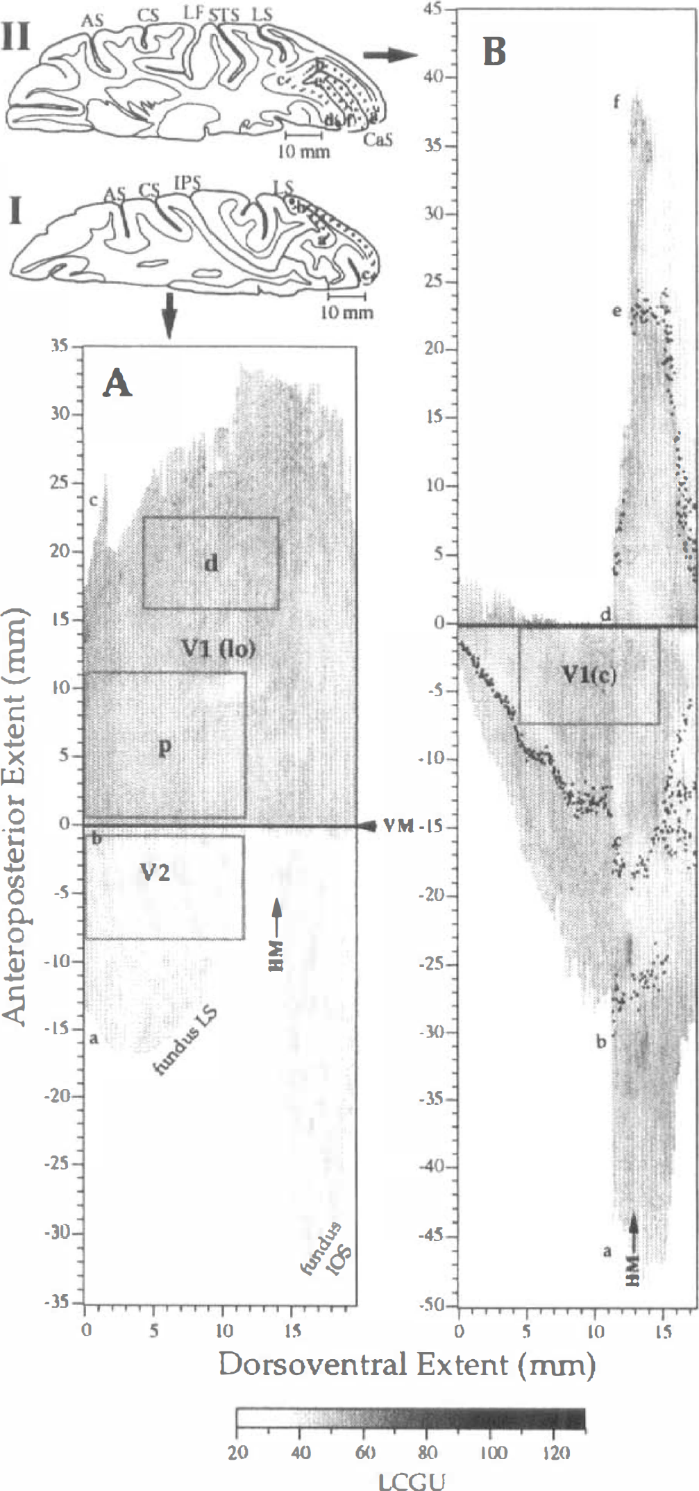
A reconstructed 2D metabolic map of the visual areas V1 lateral occipital [V1(lo)] and V2 is shown in Fig. 1A. This 2D metabolic map is derived from one hemisphere of the control animal, as described in the Materials and Methods section. Arrows on this map indicate the representation of horizontal meridian (HM) and the representation of vertical meridian (VM), which coincides with V1/V2 border (Zeki, 1969; Gattass et al., 1981). Rectangles outline the regions that were analyzed by 2D FFT. The lower rectangle (p) in area V1(lo), which has anteroposterior and dorsoventral extent of 10.8 mm and 11.4 mm, respectively, is proximal to the representation of VM and dorsal to the representation of HM. Thus, this rectangle corresponds to eccentricities of 1 to 6 degrees of the contralateral lower visual field, according to previous studies (Gattass et al., 1981; Van Essen et al., 1984). The upper rectangle (d) in V1(lo), which is distal to the representation of VM and dorsal to the representation of HM, is 6.9 × 10.4 mm and corresponds to eccentricities of 4 to 10 degrees (Gattass et al., 1981; Van Essen et al., 1984). Diagrammatic representations of our autoradiographic sections from two dorsoventral levels are shown next to the 2D maps (Fig. 1, diagrams I and II). Diagrammatic representation I illustrates how area V1(lo), which lies on the exposed lateral occipital surface, and area V2, which lies in the posterior banks of lunate and inferior occipital sulci, were unfolded. Letters a-c indicate the same landmarks in both Diagram I and 2D map A (Fig. 1). The solid circle b in the diagrammatic representation indicates the V1/V2 border. A reconstructed 2D metabolic map of intracalcarine area V1 of the control hemisphere is shown in Fig. 1B. The region that was analyzed by 2D FFT (6.9 × 9.9 mm) is outlined by the rectangle V1(c) and corresponds to eccentricities of 10 to 40 degrees (Gattass et al., 1981; Van Essen et al., 1984). Diagrammatic representation II in Fig. 1 demonstrates by serial letters (a-f) the way the intracalcarine area V1 was unfolded, measured, and reconstructed.
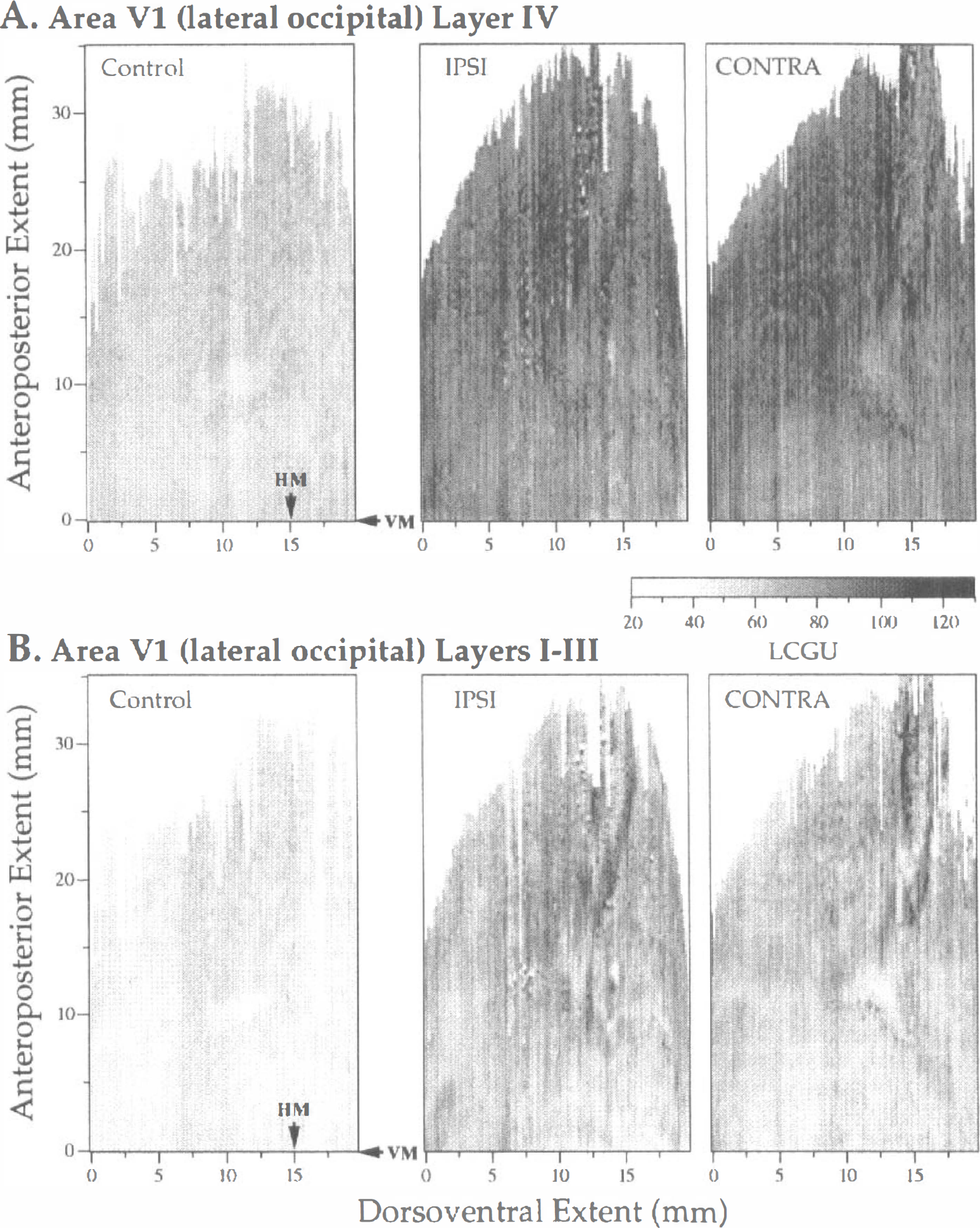
Layer IV was measured and reconstructed separately from superficial layers I through III in V1(lo) cortex (Fig. 2). Thalamorecipient layer IV of area V1 is easily distinguished in autoradiographic sections because it displays much greater metabolic activity compared with the superficial layers I through III. The 2D metabolic maps of the right hemisphere in the control monkey (Control) and the two hemispheres (IPSI, ipsilateral; CONTRA, contralateral to the visually guided forelimb) of the experimental monkey are shown in Fig. 2 (A, layer IV; B, layers I through III). The lower border of the LCGU maps in this figure coincides with the representation of VM or the V1/V2 border. The approximate representation of HM is also marked with an arrow. Only one control hemisphere is illustrated in each of our figures because both control hemispheres displayed similar maps and 2D FFT results in our study. The maps of the control monkey displayed a rather homogeneous pattern of metabolic activity that was characterized by lower LCGU values (layer IV, 56.8 ± 3.1, mean ± SD; layers I through III, 46.0 ± 3.4) than those in the experimental monkey (IPSI layer IV, 86.4 ± 7.1; IPSI layers I through III, 63.2 ± 5.9; CONTRA layer IV, 88.4 ± 5.8; CONTRA layers I through III, 59.4 ± 5.1).
The global bilateral metabolic activation of V1(lo), including its subregions of foveal and parafoveal representations of the visual field, is attributed to enhanced visual attentive processes of the experimental monkey relative to the no-task control (Savaki and Dalezios, in press). Indeed in the experimental monkey, all visual stimuli appear either in the upper left quadrant (i.e., target button) or in the lower right quadrant of the visual field (i.e., start button and moving forelimb). However, the V1(lo) cortex is not as expected specifically activated in the ventral part of the right (CONTRA) hemisphere and in the dorsal part of the left (IPSI) hemisphere, but all over its dorsoventral and anteroposterior extent in both hemispheres (Fig. 2). As regards the distribution of effects within the different layers of V1(lo), layer IV is much more activated than the upper layers I through III (Fig. 2). The higher activation in layer IV of V1, which is the site of termination of geniculate afferents (layer IVC) and contains direction-selective neurons (layer IVB), reflects enhanced input from the periphery and increased processing of visuomotion. Of interest is that no pattern of columnar organization is apparent in the LCGU maps illustrated in Fig. 2. However, a columnar pattern of cortical organization is revealed in area V1(lo) after these LCGU maps have been filtered as described in the Materials and Methods section (Figs. 3–6, left column).
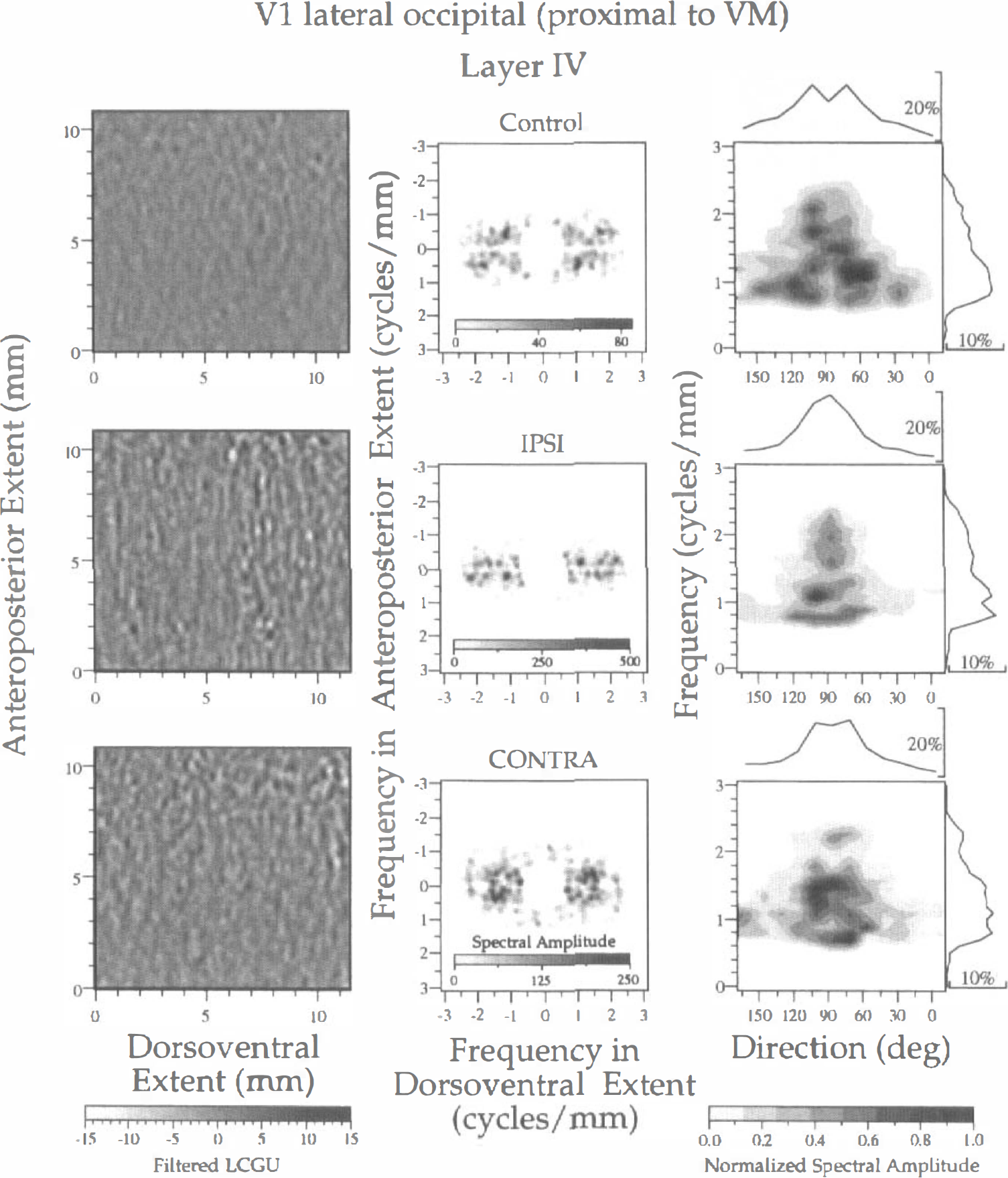
Spectral analysis of LCGU in layer IV of area V1(lo). The results of a subregion proximal to the representation of VM, outlined in Fig. 1A (rectangle p), are illustrated in one control (upper row) and two experimental (IPSI, middle row; CONTRA, lower row) hemispheres. Left column: Filtered images of the 2D maps illustrated in Fig. 2A. Each image represents a region outlined by rectangle p in Fig. 1A. The bandpass filter had a lower cutoff frequency of 0.7 cycles/mm and an upper cutoff frequency of 2.5 cycles/mm. The gray scale bar at the bottom indicates the filtered LCGU values. Middle column: Two-dimensional spectra generated after 2D FFT of the filtered images shown in the left column. The abscissa denotes the frequency (cycles/mm) across the dorsoventral dimension, and the ordinate denotes the frequency across the anteroposterior extent. A spectral amplitude scale is included within each plot. Right column: Plots of the normalized spectral amplitude versus frequency (ordinate) and direction (abscissa) of metabolically active bands. The spectral amplitudes shown in the middle column were averaged over sectors of 15 degrees with a frequency resolution of 0.1 cycles/mm. These average values were normalized by dividing them with their maximal value. The direction of the bands is defined counterclockwise with respect to the representation of VM. Curves on top of plots show the distribution of the relative spectral amplitude (defined as the percentage of the total spectral amplitude) versus direction. Curves on the right of plots show the distribution of the relative spectral amplitude versus frequency. The gray scale bar at the bottom indicates the normalized spectral amplitude.
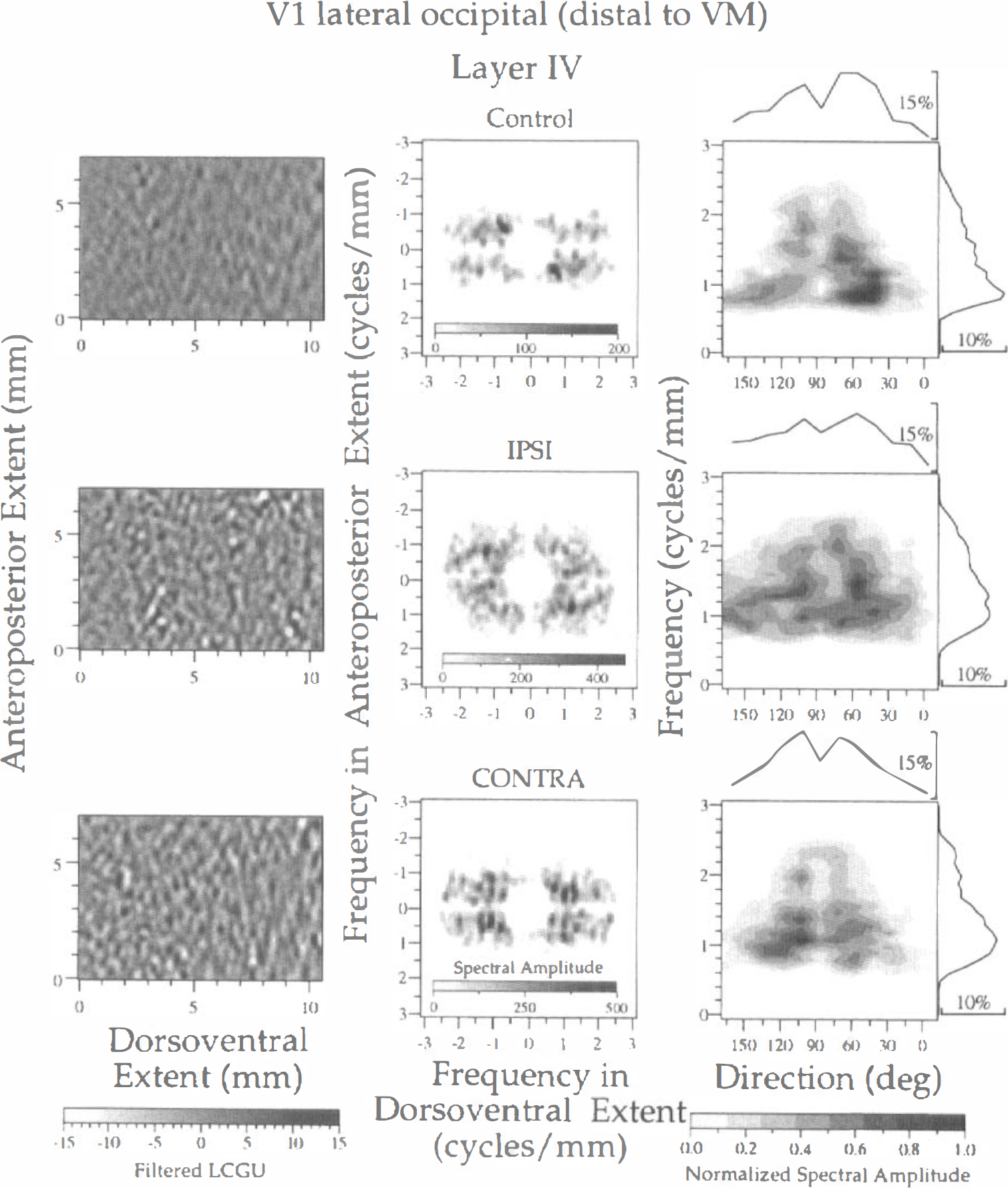
Spectral analysis of LCGU in layer IV of area V1(lo) in one control (upper row) and two experimental (IPSI, middle row; CONTRA, lower row) hemispheres. The subregion of V1(lo) that is distal to the representation of VM and outlined in Fig. 1A (rectangle d) is illustrated. Left column: Filtered images of the 2D maps presented in Fig. 2A. Each image represents a region outlined by rectangle d in Fig. 1A. Bandpass filters and gray scale bar as in Fig. 3. Middle column: Two-dimensional spectra generated after 2D FFT of the filtered images shown in the left column. The abscissa and ordinate denote frequencies (cycles/mm) across the dorsoventral and anteroposterior extent, respectively. Right column: Plots of the normalized spectral amplitude versus frequency (ordinate) and direction (abscissa) of metabolically active bands. Calculation of normalized spectral amplitude and rest of conventions as in Fig. 3.
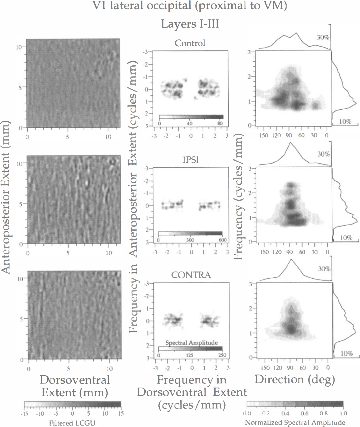
Spectral analysis of LCGU in layers I through III of area V1(lo). The subregion proximal to the representation of VM, outlined in Fig. 1A (rectangle p), is illustrated in one control (upper row) and two experimental (IPSI, middle row; CONTRA, lower row) hemispheres. Left column: Filtered images of the 2D maps illustrated in Fig. 2B. Each image represents a region outlined by rectangle p in Fig. 1A. Bandpass filters and gray scale bar as in Fig. 3. Middle column: Two-dimensional spectra generated after 2D FFT of the filtered images shown in the left column. The abscissa and ordinate denote frequencies across the dorsoventral and anteroposterior extent, respectively. Right column: Plots of the normalized spectral amplitude versus frequency (ordinate) and direction (abscissa) of metabolically active bands. Calculation of normalized spectral amplitude and rest of conventions as in Fig. 3.
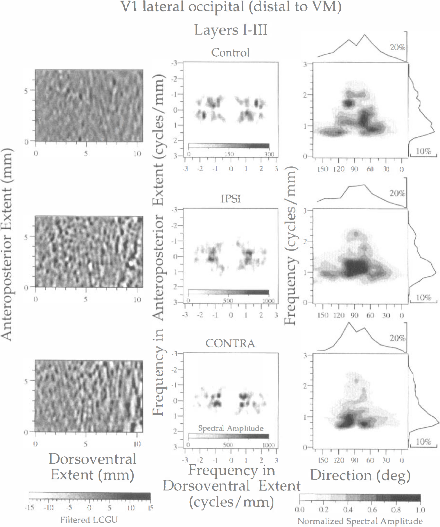
Spectral analysis of LCGU in layers I through III of area V1(lo). The subregion distal to the representation of VM, outlined in Fig. 1A (rectangle d), is illustrated in one control (upper row) and two experimental (IPSI, middle row; CONTRA, lower row) hemispheres. Left column: Filtered images of the 2D maps presented in Fig. 2B. Each image represents a region outlined by rectangle d in Fig. 1A. Bandpass filters and gray scale bar as in Fig. 3. Middle column: Two-dimensional spectra generated after 2D FFT of the filtered images shown in the left column. The abscissa and ordinate denote frequencies across the dorsoventral and anteroposterior extent, respectively. Right column: Plots of the normalized spectral amplitude versus frequency (ordinate) and direction (abscissa) of metabolically active bands. Calculation of normalized spectral amplitude and rest of conventions as in Fig. 3.
Layer IV
The results of spectral analysis of layer IV in a V1(lo) subregion proximal to the V1/V2 border (as outlined by rectangle p, Fig. 1A) are illustrated in Fig. 3. In this figure, rows represent hemispheres (control, IPSI, CONTRA), and columns represent different steps of the spectral analysis. The left column of Fig. 3 illustrates filtered images from the 2D maps presented in Fig. 2A. Given that the periodicities of the columnar systems in the striate cortex reported in the literature range between 1,300 and 500 μm (Crawford, 1984; Tootell et al., 1988a; Obermayer and Blasdel, 1993; Löwel, 1994; Horton and Hocking, 1996a), the bandpass filter used for all the examined V1 subregions had a lower cutoff frequency of 0.7 cycles/mm and an upper cutoff frequency of 2.5 cycles/mm, corresponding to periods of 1.43 and 0.4 mm, respectively. In these filtered images it is apparent that alternating bands of high and low metabolic activity are present in the control and the experimental hemispheres. These bands run almost perpendicular to the V1/V2 border (which is parallel to the abscissa) and present bifurcations and blind endings at various intervals. The contrast between bands of high and low metabolic activity is greater in the two hemispheres of the experimental monkey than in the control hemisphere (Fig. 3, gray scale at the bottom of the left column). Dots of enhanced metabolic activity are superimposed on the active bands in all three hemispheres, although they are more pronounced in the experimental ones (Fig. 3, left column).
The middle column of Fig. 3 shows the spectra generated after 2D FFT of the filtered LCGU images in the left column of the same figure. These spectra display noisy symmetrical peaks whose axis is perpendicular to the direction of the bands. The frequency along this axis represents the center-to-center distance of the bands in this direction. The abscissa denotes symmetrical frequency values (in cycles per millimeter) along the dorsoventral extent (zero lag at the center), and the ordinate denotes the frequency along the anteroposterior extent of the LCGU maps. The spectral amplitude is given in intensities of a gray scale (Fig. 3, insets in middle column). The most pronounced difference among the spectra of the three hemispheres concerns their amplitudes (note that each gray scale represents a different range of values). The maximal spectral amplitude in the control hemisphere is 3 to 6 times lower than that in the experimental hemispheres. This difference may be related to (1) lower LCGU values in area V1 of the control monkey as compared with those in the experimental one and or (2) a diffusion of the spectral density along various frequencies and directions in the control hemisphere as compared with the experimental one. The latter possibility could suggest a better organization of functional bands in the visually stimulated striate cortex.
Differences in LCGU values between the control and experimental hemispheres are squared after spectral analysis. To eliminate the effect of LCGU differences we normalized the spectral amplitude as follows. We averaged the values of spectral amplitude over sectors of 15 degrees (directions differing by 180 degrees were averaged together) with a frequency resolution of 0.1 cycles/mm. The average value in each sector was normalized by dividing it with the maximal value obtained after the averaging procedure. The right column in Fig. 3 displays plots of the normalized spectral amplitude versus (1) the frequency (ordinate) and (2) the direction of the long axis of bands (abscissa). The direction is defined counterclockwise with respect to the V1/V2 border. Zero value corresponds to bands that run parallel to this border, and values of 90 degrees correspond to bands running perpendicular to it. The values of normalized spectral amplitude are indicated by a gray scale bar below the right column (Fig. 3). The surface of each dark area is inversely related to the sharpness of the corresponding peak. The normalized peak values and their corresponding frequencies, periods, and directions are presented in Table 1. In the same table, an index of the sharpness of each peak is provided. Sharpness is defined as the ratio of the amplitude of a peak versus the average of its eight adjacent amplitudes in the grid defined by the direction and frequency axes. Given that the sampling procedure is identical in all three hemispheres, the sharpness is an index of the spectral variability in frequencies and directions. Thus, high values of sharpness indicate peaks well defined at a specific frequency and direction whereas low values indicate shallow peaks. Curves on top of plots (Fig. 3, right column) show the distribution of the relative spectral amplitude (defined as the percentage of the total spectral amplitude) along all directions and independent of frequency. Curves on the right of plots show the distribution of the relative spectral amplitude along all frequencies and independent of direction.
Characteristics of the normalized spectra obtained after 2D-FFT of the LCGU values in visual areas of one control and two experimental hemispheres
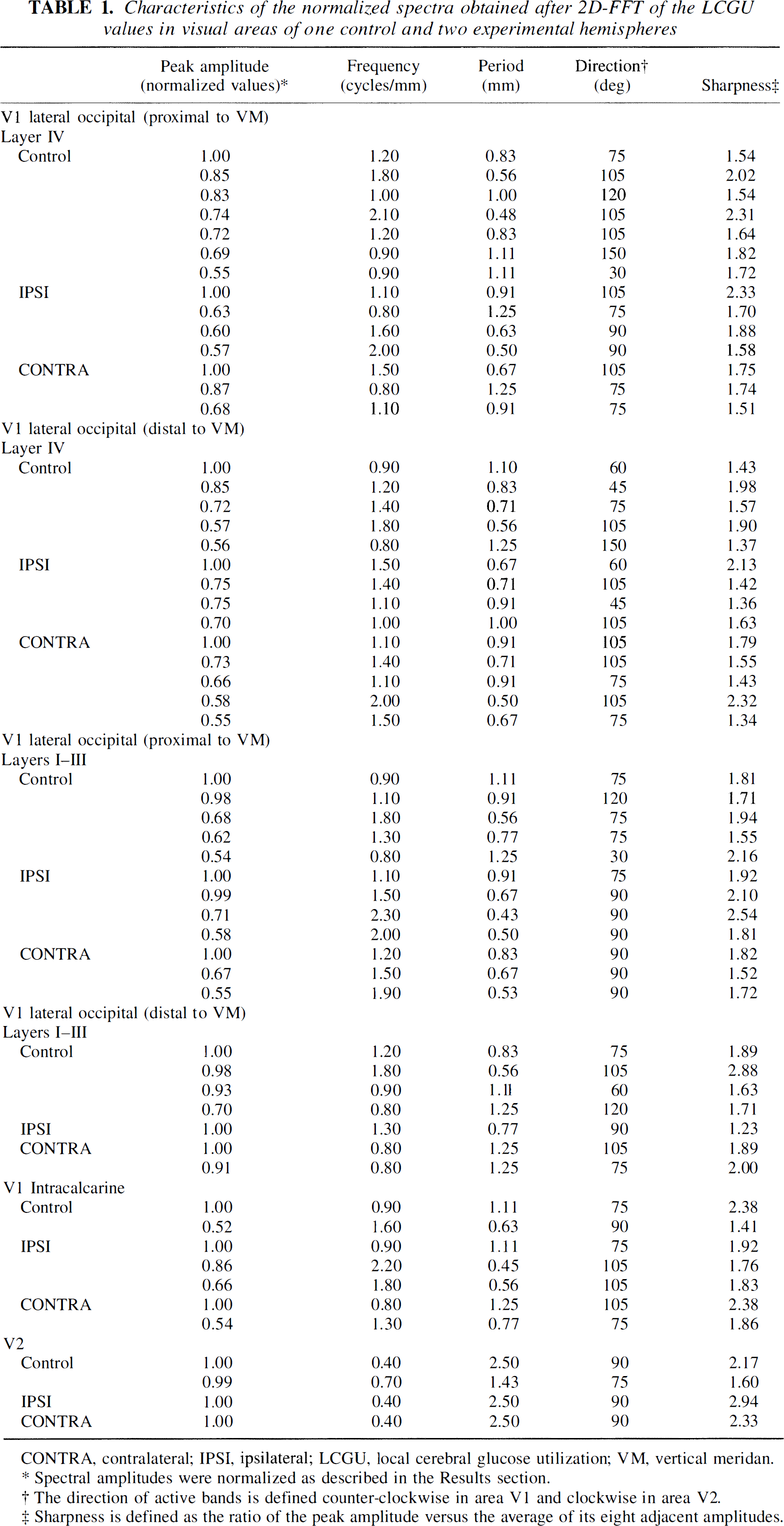
CONTRA, contralateral; IPSI, ipsilateral; LCGU, local cerebral glucose utilization; VM, vertical meridan.
Spectral amplitudes were normalized as described in the Results section.
The direction of active bands is defined counter-clockwise in area V1 and clockwise in area V2.
Sharpness is defined as the ratio of the peak amplitude versus the average of its eight adjacent amplitudes.
The above mentioned analysis revealed that in the control hemisphere the bands run in various directions, ranging between 30 and 150 degrees. These bands have different center-to-center distances, ranging between 0.48 and 1.11 mm (Fig. 3, right column; Table 1). The large number of peaks with values close to maximum, as well as the broad range of directions and frequencies of bands, indicates a poor organization of the activity pattern in the control hemisphere. In contrast, the two experimental hemispheres are characterized by peaks within a narrow range of directions (75 to 105 degrees), although the range of their periods is similar to that of the control hemisphere (0.5 to 1.25 mm). The fewer and sharper peaks in combination with a smaller range of directions in the experimental as compared with the control hemispheres indicate a better organized pattern of activity in layer IV of the V1(lo) region that is proximal to the representation of VM after visual stimulation.
As regards the region of V1(lo) that is distal to the representation of VM (Fig. 1A, rectangle d), the same type of analysis of the LCGU values gave results similar to those described above. The contrast between bands of high and low metabolic activity is more pronounced in the experimental (IPSI and CONTRA) hemispheres than in the control one (Fig. 4, left column). However, the active bands in the filtered images of this subregion distal to the representation of VM (Fig. 4, left column) appear more spotty than those in the subregion proximal to the representation of VM (Fig. 3, left column). This is in agreement with an earlier observation in area V1 that rows of columns close to the V1/V2 border become rows of spots further away (Crawford, 1984). The spectra generated after 2D FFT of LCGU values in the region distal to the V1/V2 border are more noisy (Fig. 4, middle column) than the corresponding spectra of the region proximal to the same border (Fig. 3, middle column). The most pronounced difference between the spectra of the control and the experimental hemispheres concerns their amplitudes. The maximal amplitude in the control hemisphere is 2 to 2.5 times lower than that of the experimental hemispheres (Fig. 4, right column). When the normalized amplitude is plotted versus the frequency and the direction of the long axis of bands, the control hemisphere shows an irregular pattern of organization. The bands in the control hemisphere run in directions ranging between 45 and 150 degrees and their center-to-center distances range between 0.56 and 1.25 mm (Fig. 4, right column; Table 1). In the experimental hemispheres, the direction of bands ranges between 45 and 105 degrees and their periods range between 0.5 and 1.0 mm.
A common finding in layer IV of both subregions (proximal and distal to the representation of VM) examined within area V1(lo) is that bands with similar periodicities intersect each other at angles ranging between 45 and 60 degrees (Figs. 3 and 4, plots in right column; Table 1). This intersection is represented by the two peaks in the graphs illustrating the distribution of the relative spectral amplitude versus the direction of bands (Figs. 3 and 4, curves on top of plots in right column).
Layers I through III
The results of spectral analysis of LCGU values in the superficial cortical layers I through III in the V1(lo) subregion that is proximal to the V1/V2 border (Fig. 1A, rectangle p) are illustrated in Fig. 5. As in the corresponding images of layer IV (Fig. 3, left column), the filtered images generated from the 2D metabolic maps demonstrate a higher contrast in layers I through III of the experimental hemispheres than those in the control hemisphere (Fig. 5, left column). Dots of enhanced metabolic activity are superimposed on the active bands in the filtered images of the control and the experimental hemispheres. The spectra generated after 2D FFT of the filtered LCGU images display symmetrical peaks that lie mainly in one axis of symmetry (Fig. 5, middle column). However, the bands of the control hemisphere are scattered over a wider range of directions (30 to 120 degrees) than those of the experimental hemispheres, which run practically in one direction (90 degrees), i.e., normal to the V1/V2 border (Fig. 5, right column; Table 1). The periods display an average of 0.92 and 0.65 mm in the control and experimental hemispheres, respectively. In summary, the diffused organization of the metabolically active bands in the superficial layers I through III of the control hemisphere results mainly from a spread in directions of bands, similar to layer IV.
Similar results were obtained after 2D FFT of LCGU values in layers I through III within the V1(lo) subregion that is distal to the representation of VM and outlined by rectangle d in Fig. 1A. The filtered images produced from the 2D metabolic maps demonstrate a higher contrast in the experimental than in the control hemisphere (Fig. 6, left column). The spectra generated after 2D FFT of the filtered LCGU images are aligned around one axis of symmetry, which reflects bands almost perpendicular to the V1/V2 border (Fig. 6, middle column). The spectrum of the control hemisphere displays four major peaks in different directions (60, 75, 105, and 120 degrees). The experimental hemispheres display one (IPSI) and two (CONTRA) major peaks that correspond to band directions of 90 degrees for the ipsilateral and 75 and 105 degrees for the contralateral hemisphere (Fig. 6, right column; Table 1). The periods of the bands range between 0.56 and 1.25 mm in the control hemisphere. In the experimental hemispheres, the estimated periods are 0.8 mm in the ipsilateral and 1.25 mm in the contralateral hemisphere. However, given that the peak in the ipsilateral hemisphere is very shallow (see sharpness in Table 1), the period of active bands in this hemisphere should be considered to range between 0.8 and 1.0 mm (Fig 6, right column, curve on the right of middle plot).
After spectral analysis, the main difference observed between layer IV and superficial layers I through III in area V1(lo) regards the direction of the long axis of active bands. In layers I through III most bands run mainly perpendicular to the V1/V2 border (Figs. 5 and 6), whereas in layer IV two sets of bands with similar periodicities intersect each other at angles of 45 to 60 degrees (Figs. 3 and 4; Table 1).
Intracalcarine visual cortex
The region within intracalcarine area V1 analyzed by 2D FFT [Fig. 1B, rectangle V1(c)] corresponds to eccentricities of 10 to 40 degrees (Van Essen et al., 1984). The LCGU in all layers was averaged pixel by pixel and processed for spectral analysis, as described in the Materials and Methods section. The applied bandpass filter was the same as that used for area V1(lo). The filtered images in area V1(c) (Fig. 7, left column) display a pattern of metabolic activity that is more irregular than the corresponding patterns in the examined subregions of area V1(lo) (Figs. 3–6, left column). The spectra generated after 2D FFT do not differ in maximal amplitude values between the control and the experimental hemispheres (Fig. 7, middle column). The plots of normalized amplitude versus frequency and direction of bands reveal that the bands run in directions ranging between 75 and 105 degrees and the periods range between 0.45 and 1.25 mm (Fig. 7, right column; Table 1). Of interest is the finding that in the visually stimulated hemispheres, the average main period of active bands estimated within V1(c), which represents peripheral vision, is greater than that estimated in V1(lo) area, which represents foveal and parafoveal central vision (1.18 mm versus 0.87 mm).
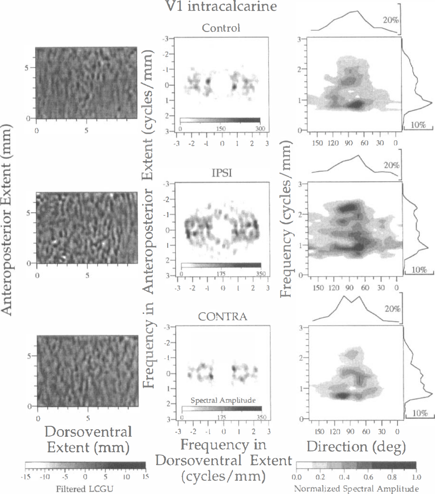
Spectral analysis of LCGU in the whole laminar thickness of intracalcarine V1 cortex in one control (upper row) and two experimental (IPSI, middle row; CONTRA, lower row) hemispheres. Left column: Filtered images of 2D maps. Each image represents a region outlined by rectangle V1(c) in Fig. 1B. Bandpass filters and gray scale bar as in Fig. 3. Middle column: Two-dimensional spectra generated after 2D FFT of the filtered images shown in the left column. The abscissa and ordinate denote frequencies across the dorsoventral and anteroposterior extent, respectively. Right column: Plot of the normalized spectral amplitude versus frequency (ordinate) and direction (abscissa) of metabolically active bands. Calculation of normalized spectral amplitude and rest of conventions as in Fig. 3.
Area V2
The thick and thin stripes of area V2 extend across all cortical layers (Tootell and Hamilton, 1989). For this reason, we did not treat the superficial layers separately from layer IV. The region that was analyzed by 2D FFT is outlined in Fig. 1A by a rectangle of 7.4 mm anteroposterior × 11.4 mm dorsoventral extent. A stripelike pattern is apparent in area V2 by visual inspection of the 2D metabolic map even before filtering it (Fig. 1A). The bandpass filter that was used in area V2 and a lower cutoff frequency of 0.25 cycles/mm (period of 4.0 mm) and an upper cutoff frequency of 2.5 cycles/mm (period of 0.4 mm). As illustrated in Fig. 8 (left column) the stripes have a curvilinear shape and run almost perpendicular to the representation of VM near the V1/V2 border. Patches of high metabolic activity are superimposed on these stripes. The spectra generated after 2D FFT of LCGU values in area V2 (Fig. 8, middle column) are in general less diffused than those in area V1 (Figs. 3–7). However, the spectrum of the control hemisphere is more noisy than those in the experimental hemispheres, similar to area V1. This is obvious in the plots of normalized spectral amplitude versus frequency and direction of stripes defined clockwise with respect to the V1/V2 border (Fig. 8, right column). In the control hemisphere, the spectral amplitude is spread between two main frequencies, which correspond to periods of 1.43 and 2.5 mm (Fig. 8, right column; Table 1). In the experimental hemispheres, the stripes have a main center-to-center distance of 2.5 mm and their peaks are very sharp. The spread over directions is because of the curvilinear shape of the stripes. The stripes are almost perpendicular to the V1/V2 border, and they run in a direction decreasing from 90 to 60 degrees as their distance from this border increases (Fig. 8, left column).
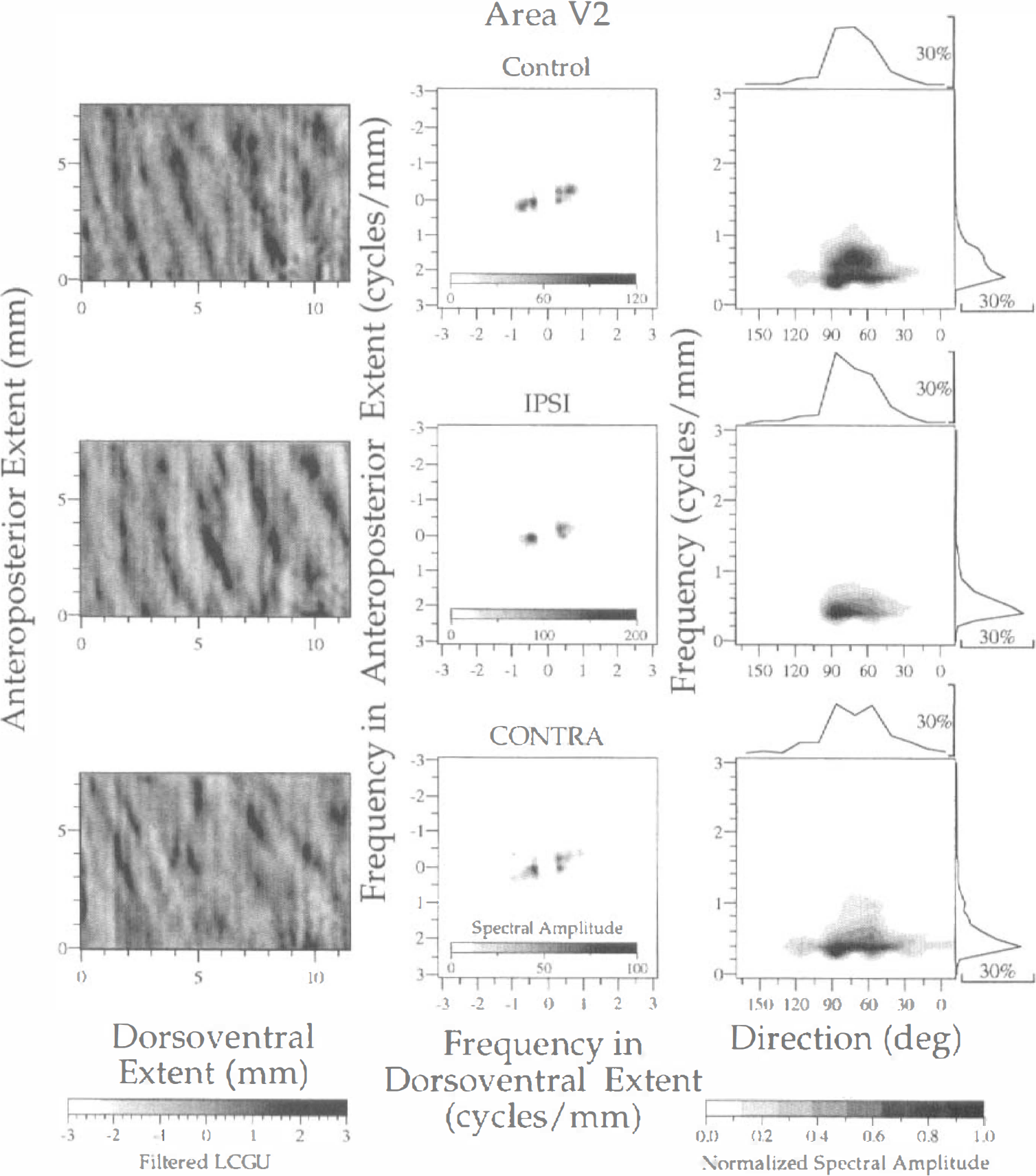
Spectral analysis of LCGU in the whole laminar thickness of area V2 in the control (upper row) and the experimental (IPSI, middle row; CONTRA, lower row) hemispheres. Left column: Filtered images of the 2D maps. Each image represents a region outlined by the rectangle V2 in Fig. 1A. The bandpass filter had a lower cutoff frequency of 0.25 cycles/mm and an upper cutoff frequency of 2.5 cycles/mm. The gray scale bar at the bottom indicates the filtered LCGU values. Middle column: Two-dimensional spectra generated after 2D FFT of the filtered images shown in the left column. The abscissa denotes frequencies across the dorsoventral dimension, and the ordinate denotes frequencies across the anteroposterior extent. A spectral amplitude scale is included within each plot. Right column: Plots of the normalized spectral amplitude versus frequency (ordinate) and direction (abscissa) of metabolically active bands. The normalized spectral amplitude was calculated as described in Fig. 3. The direction of active bands is defined clockwise with respect to the representation of VM. Calculation of normalized spectral amplitude and rest of conventions as in Fig. 3.
DISCUSSION
Methodological considerations
The present study is the first to analyze quantitatively the parameters that characterize the spatial pattern of metabolic activity in the monkey visual cortex during the presentation of behaviorally important visual stimuli. Previous electrophysiologic, anatomic, and imaging studies have described the organization of the visual cortex into ocular dominance and orientation columns, and color blobs (Hubel and Wiesel, 1977; Crawford et al., 1982; Livingstone and Hubel, 1982; Tootell et al., 1982, 1983, 1988a, 1988b, 1988c, 1988d; Humphrey and Hendrickson, 1983; Crawford, 1984; Friedman et al., 1989). These studies have used anesthetized, paralyzed preparations and thus their conclusions do not necessarily apply to alert subjects. The 14C-DG quantitative brain imaging is a powerful noninvasive method for the study of functional cortical activity in alert behaving animals. Furthermore, this method maps the local metabolic activity in the entire cortex simultaneously whereas the classic single-cell recording techniques are restricted to one cell and one area at a time (Sokoloff et al., 1989). Finally, the advantage of the 14C-DG quantitative method over the optical imaging method is its ability to map the activity of cortical areas that lie inside the cerebral sulci. However, in contrast to single-cell recording and optical imaging techniques, the 14C-DG method cannot provide information about the cerebral effects of different experimental conditions in the same animal. This disadvantage is minimized when the 2D reconstructed maps of activity pattern are generated in both the experimental brain and its appropriate control, and an experimental minus control image is constructed (Dalezios et al., 1996; Savaki et al., 1997). Finally, the double-labeling (14C and 3H) DG method can also provide information about the cerebral effect of different experimental conditions in the same animal (Friedman et al., 1989), but it is prone to interpretative difficulties because of its qualitative character.
Previous metabolic studies relied on visual inspection of autoradiographic sections to provide a quantitative description of the spatial arrangement of the columnar systems in the striate visual cortex. This also applies to previous reports of the distance between adjacent columns (Hubel et al., 1977; Crawford et al., 1982; Humphrey and Hendrickson, 1983; Crawford, 1984; Herdman et al., 1984; Tootell et al., 1988a; Savaki et al., 1993). This approach may be valid when the visual stimuli activate only one particular columnar system, e.g., either eye preference or orientation columns. However, when the visual stimuli activate more than one columnar systems as in our alert behaving monkeys, active bands (or columns) of different periodicities may overlap each other, thus obscuring any estimate based on visual inspection. In this case, a proper mathematical treatment such as the 2D FFT is required to obtain accurate results about (1) the existence of columnar periodicities, (2) the direction of the long axis of each activated columnar system, and (3) the minimal distance between adjacent columns (Obermayer et al., 1992; Obermayer and Blasdel, 1993). So far, it is only the one-dimensional FFT that has been used in a 14C-DG study of the columnar organization in the cat visual cortex (Löwel et al., 1988; Löwel, 1994). The problem with the one-dimensional FFT is that it does not necessarily provide the minimal distance between adjacent columns, unless it is performed along the direction perpendicular to their long axis, which is unknown. This is the reason why we chose the 2D FFT to analyze the pattern of metabolic activity in visual areas V1 and V2 in the present study.
Area V1
Visual inspection of the 14C-DG reconstructed metabolic maps in the present study indicates a rather uniform distribution of metabolic activity in area V1 (Fig. 2) as illustrated in our previous study (Savaki et al., 1997). However, when the images of the 14C-DG metabolic maps are filtered, a pattern of alternating bands of high and low metabolic activity is revealed (Figs. 3–7, left column) that resembles that of columnar arrangements previously described within area V1 (Hubel and Wiesel, 1977; Hubel et al., 1978; Tootell et al., 1988a; Horton and Hocking, 1996a). In the filtered images, it becomes apparent that the contrast between bands of high and low metabolic activity is greater in the experimental than in the control hemispheres. Presumably, this enhancement of contrast is caused by the activation of V1 by visual stimuli presented to the experimental monkeys (Savaki et al., 1993, 1997). Moreover, both the autoradiographic sections and the 14C-DG metabolic maps display higher LCGU values in layer IV than in the superficial layers, in agreement with previous reports (Hubel et al., 1977, 1978; Humphrey and Hendrickson, 1983; Tootell et al., 1988a; Savaki et al., 1993). Subsequent spectral analysis of the filtered images reveals a distinct arrangement of metabolically active bands, characterized by specific frequencies and directions. Thus, our approach reveals patterns of metabolically active bands that cannot be detected by visual inspection alone. Finally, normalization of the spectral amplitude demonstrates that the spatial pattern of the metabolically active bands is more organized in the experimental than in the control hemispheres, in terms of periods and directions (Table 1; Figs. 3–7, middle and right columns). This finding reflects an effect on the columnar organization in area V1, which is induced by the presentation of behaviorally important visual stimuli. Thus, it is suggested that visual stimulation induces in the striate cortex activation of columnar arrangements, which emerge from the underlying complex network of columnar systems constituting the visual cortex.
Two-dimensional FFT of LCGU values in area V1(lo) of the experimental monkey demonstrates metabolically active bands with an average main period of 0.87 mm, and main directions of 45 to 105 degrees in layer IV and 90 to 105 degrees in layers I through III counterclockwise with respect to the representation of VM. The main periods of active bands in area V1 of the visually stimulated monkey, which were estimated by spectral analysis in the present study, range between 0.67 and 1.25 mm. This range of periods is in agreement with that reported earlier (0.6 to 1.3 mm) for the ocular dominance (Löwel et al., 1988; Tootell et al., 1988a; Blasdel, 1992a; Obermayer and Blasdel, 1993; Horton and Hocking, 1996b) and the orientation columns (Hubel et al., 1977, 1978; Löwel et al., 1988; Obermayer and Blasdel, 1993). Moreover, the ocular dominance and the orientation columns are reported to have similar periods when examined in the same animal (Löwel et al., 1988; Obermayer and Blasdel, 1993). Accordingly, it is difficult to discriminate between active bands representing ocular dominance columns and bands representing orientation columns with the spectral analysis of the present study.
In our study, the orientation columns may have been activated because of the exposure of our experimental monkey to a virtual linear segment directed 135 degrees counterclockwise from the horizontal plane. This virtual stimulus results from the successive onset of the central and peripheral visual targets. Moreover, although the visual stimulation is binocular in our study, the ocular dominance columns may also have been activated in the experimental monkey. Activation of ocular dominance columns during binocular stimulation is caused by the unequal representation of the two eyes in the two hemispheres. In V1 area of each hemisphere the columns of the contralateral eye are less distinct because of a high intercolumnar projection, whereas those of the ipsilateral eye are sharply delineated and occupy a slightly smaller area of the hemisphere (Anderson et al., 1988; Horton and Hocking, 1996a). In a previous study, 14C-DG labeling of the orientation columns was demonstrated in layers IVCa and IVB of area V1 whereas labeling of the ocular dominance columns was shown in layers IVCb and IVA (Tootell et al., 1988a). Given that in our study all the subdivisions of layer IV were averaged together pixel by pixel, the wide range in directions of the long axis of active bands (45 to 105 degrees) may reflect the coactivation of the ocular dominance and orientation columnar systems in this layer. This suggestion is further supported by our finding that bands with similar periodicities cross each other at angles ranging between 45 and 60 degrees (Table 1; Figs. 3, 4), a finding that is consistent with previous reports concerning the angles of intersection between orientation and ocular dominance columns (Tootell et al., 1988a; Obermayer and Blasdel, 1993; Hübener et al., 1997).
As regards the superficial layers I through III of area V1, spectral analysis reveals that the active bands in the experimental monkey run mainly in one direction ranging between 90 and 105 degrees counterclockwise with respect to the representation of VM (Figs. 5 and 6). We suggest that these bands represent the activated orientation columns because according to previous studies it is mainly the orientation columns that are labeled by 14C-DG in the superficial layers of area V1 (Hubel et al., 1977, 1978; Humphrey and Hendrickson, 1983; Tootell et al., 1988a), in contrast to the ocular dominance columns, which are labeled by 14C-DG mainly in the thalamorecipient layer IV of the striate cortex (Löwel et al., 1988; Tootell et al., 1988a; Blasdel, 1992a).
Another finding of the spectral analysis in our study is that the average main period in area V1(lo) that subserves foveal and parafoveal vision (0.87 mm) is smaller than the period in area V1(c) that subserves peripheral vision (1.18 mm). This finding is compatible with a previous 14C-DG qualitative observation that the spacing between the stimulus-specific columns in striate cortex is narrowest for the foveal representation and increases at peripheral field representations (Crawford, 1984). The generalized increase in glucose consumption within both V1 areas of central and peripheral visual representations in the experimental as compared with the control monkey may be associated with the increased visual attention in the performing subject as previously suggested (Savaki et al., 1997). Finally, the more organized active bands in V1 area of central visual representation (Figs. 3–6) than in V1 area of peripheral visual representation (Fig. 7) in the experimental subject may be associated with increased information processing within the parts of V1 where central vision is represented.
Area V2
The stripelike pattern of primate area V2 has been demonstrated in the past by anatomic, electrophysiologic, and metabolic methods (Tootell et al., 1983; DeYoe and Van Essen, 1985; Hubel and Livingstone, 1987). The thick and thin stripes and the pale interstripes receive different inputs from area V1 and process different visual modalities, such as direction, color, and orientation (Hubel and Livingstone, 1987). However, in area V2 of the macaque monkey the distinction between thick and thin stripes is not obvious based on size alone (Olavarria and Van Essen, 1997). The main period estimated by spectral analysis within area V2 in the present study is 2.5 mm and the direction of the long axis of active bands ranges between 75 and 90 degrees clockwise from the representation of VM, i.e., the V1/V2 border (Table 1; Fig. 8). This directional range reflects the curvilinear shape of active bands in V2, which is apparent in the filtered images (Fig. 8, left column). Our findings that the stripes within dorsal area V2 extend up to 10 mm in length, are roughly orthogonal to the borders of area V2, and have a period of 2.5 mm are in agreement with a previous report (Olavarria and Van Essen, 1997). As in area V1, the control hemisphere displays a wider range of periods and directions of active bands as compared with the experimental hemispheres.
This finding further supports our suggestion that the active bands observed in V1 and V2 of the experimental monkey are induced by the presentation of behaviorally important visual stimuli and emerge from the underlying diffusely organized background network of activity patterns in the control state. The fact that the columns detected by spectral analysis are revealed by the presentation of behaviorally relevant visual stimuli does not necessarily mean that these columns are also task specific. It seems that in hierarchically lower cortices (e.g., within area V1) the columnar sets detected by spectral analysis of the local metabolic pattern (e.g., the ocular dominance and the orientation columns) are not task specific. They may be simply revealed by the task because of an increase in signal to noise ratio, which is related to the involvement of the experimental subject to a well controlled behavior (including behaviorally relevant visual stimulation). However, any columnar arrangements possibly detected in higher association areas may be specific to the behavioral task under performance.
In summary, the present method of analysis demonstrates two main sets of active bands within layer IV of area V1 in the experimental monkey. On the basis of periods and directions of the long axis of active bands it is suggested that one set of bands represents ocular dominance columns whereas the other set represents orientation columns. Two-dimensional spectral analysis further demonstrates one set of active bands within the superficial layers I through III of area V1 in the experimental monkey, which most probably reflects the orientation columns. Also, this method demonstrates that the period of active bands is greater in V1 area of peripheral visual representation than in V1 area of central visual representation. Finally, spectral analysis demonstrates one set of metabolically active bands in area V2 that from the period and the direction of its long axis, represents the local system of thick and thin stripes. Most of these active bands would remain undetected had we not used the 2D FFT to analyze our reconstructed metabolic brain maps.
The present results, which are in agreement with previous anatomic and functional findings in the visual cortex of anesthetized, paralyzed animals, demonstrate that spectral analysis of the metabolic activity pattern in the visual cortex of the alert behaving monkey is a valid approach. This methodological approach is potentially very powerful and is applicable to other brain regions involved in the processing of other complex information sets. Use of this method to analyze images obtained with techniques other than the 14C-DG, such as positron emission tomography and functional magnetic resonance imaging, may reveal additional important patterns of functional activity that otherwise would remain undetected.
Footnotes
Acknowledgments
The authors thank Roberto Caminiti for allowing us to use his laboratory in Universita degli Studi di Roma “La Sapienza” for part of our study. The authors also thank Vassilis Raos, Catherine Dermon, and Stefano Ferraina for technical assistance, and Yves Burnod, Constantine Christakos, Emmanuel Guigon, and Adonis Moschovakis for constructive comments.