Sage Journals: Discover world-class research

Abstract

To describe the effect of endogenous dopamine on [¹¹C]raclopride binding, we previously extended the conventional receptor ligand model to include dynamic changes in neurotransmitter concentration. Here, we apply the extended model in simulations of neurotransmitter competition studies using either bolus or bolus-plus-infusion (B/I) tracer delivery. The purpose of this study was (1) to develop an interpretation of the measured change in tracer binding in terms of underlying neurotransmitter changes, and (2) to determine tracer characteristics that maximize sensitivity to neurotransmitter release. A wide range of kinetic parameters was tested based on existing reversible positron emission tomography tracers. In simulations of bolus studies, the percent reduction in distribution volume (ΔV) caused by a neurotransmitter pulse was calculated. For B/I simulations, equilibrium was assumed, and the maximum percent reduction in tissue concentration (ΔC) after neurotransmitter release was calculated. Both ΔV and ΔC were strongly correlated with the integral of the neurotransmitter pulse. The values of ΔV and ΔC were highly dependent on the kinetic properties of the tracer in tissue, and ΔV could be characterized in terms of the tissue free tracer concentration. The value of ΔV was typically maximized for binding potentials of ~3 to 10, with ΔC being maximized at binding potentials of ~1 to 2. Both measures increased with faster tissue-to-blood clearance of tracer and lower nonspecific binding. These simulations provide a guideline for interpreting the results of neurotransmitter release studies and for selecting radiotracers and experimental design.

Keywords

Compartmental modeling Receptor binding Neurotransmitters

The binding of neuroreceptor ligands is sensitive to competition with endogenous neurotransmitter. This effect has been demonstrated in positron emission tomography (PET) and single photon emission computed tomography (SPECT) studies, which have shown that stimulation of neurotransmitter release produces a decrease in the binding of neuroreceptor ligands (Dewey et al., 1991; Innis et al., 1992; Volkow et al., 1994; Laruelle et al., 1997). In these studies of neurotransmitter competition, tracer is delivered either as two bolus injections, i.e., control and stimulus (Logan et al., 1991), or as a single bolus plus infusion (B/I) (Carson et al., 1997). With either delivery method, the change in tracer binding caused by a change in neurotransmitter level can be measured. With these techniques, tracers with different kinetic characteristics (e.g., high or low binding affinity), have shown sensitivity to endogenous neurotransmitter. Measurement of the dynamic neurotransmitter concentration in vivo has shown more directly that a change in tracer binding is caused by a change in neurotransmitter level. Microdialysis of the rat striatum showed that either an increase or decrease in neurotransmitter concentration corresponds to an opposing change in [¹¹C]raclopride binding observed in primate PET studies using the bolus technique (Dewey et al., 1995). Simultaneous measurement of dopamine and [¹¹C]raclopride in combined microdialysis-PET studies in monkeys similarly showed a decrease in [¹¹C]raclopride binding after amphetamine-stimulated dopamine release in B/I studies (Endres et al., 1997). Furthermore, a larger amphetamine dose produced a larger increase in dopamine, and a larger percent decrease in [¹¹C]raclopride concentration (Breier et al., 1997). These results suggest that a measured change in tracer binding may provide quantitative information about the underlying neurotransmitter pulse.

To better interpret studies of neurotransmitter competition, it would be useful to characterize the relation between changes in tracer binding and neurotransmitter release. Logan et al. (1991) considered the effect of a dopamine pulse on the distribution volume of [¹⁸F]-N-methylspiroperidol in bolus injection studies. The dopamine pulse was defined by its initial peak and clearance rate. Compared to a control study (i.e., with no dopamine pulse), simulations showed that a larger peak and a slower dopamine clearance rate resulted in a larger change in the tracer uptake rate as measured by graphical analysis. Furthermore, the largest effect occurred when the dopamine pulse was initiated simultaneously with tracer injection. Morris et al. (1995) performed simulations to determine the kinetic characteristics of a D₂ ligand that would have maximal sensitivity to a transient increase in dopamine. In this study, the effect of the dopamine pulse was evaluated as the sum of the squared differences in time-activity curves between a control study and a dopamine release study. From this measure, it was proposed that a completely irreversible tracer gives maximum response to a dopamine pulse.

Recently, combined PET-microdialysis experiments were performed that gave simultaneous measurements of [¹¹C]raclopride and extracellular dopamine in rhesus monkeys (Breier et al., 1997). Bolus-plus-infusion tracer delivery was used with amphetamine challenge to induce dopamine release. The data were used to extend the conventional receptor ligand model to describe the effect of endogenous dopamine on the binding of [¹¹C]raclopride (Endres et al., 1997). Initial simulations using the extended model showed that the change in [¹¹C]raclopride concentration measured with the B/I method is proportional to the integral of the amphetamine-induced dopamine pulse. This result provides a basis for the interpretation of a measured change in [¹¹C]raclopride concentration in terms of dopamine release.

In this paper, we further apply the extended model in simulations of both the bolus and B/I methods to predict the effect of neurotransmitter competition for receptor binding tracers with different kinetic properties. A wide range of tracer kinetic parameters was simulated covering established reversible PET tracers. Two specific issues were addressed: (1) determining an appropriate interpretation of the measured change in tracer binding in terms of dynamic changes in neurotransmitter concentration; and (2) examining how the kinetic characteristics of the tracer, i.e., binding constants, delivery, and nonspecific binding, affect the sensitivity to neurotransmitter concentration.

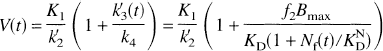
METHODS

Study overview

The model used for simulations (Fig. 1) was developed by extending the conventional two-tissue compartment model for [¹¹C]raclopride (Farde et al., 1989). One compartment represents tracer that is free or nonspecifically bound, and the second compartment represents specific binding to receptors. It is assumed that nonspecifically bound tracer is in rapid equilibrium with free tracer. The extended model also assumes rapid equilibrium between free and bound neurotransmitter, and that neurotransmitter binds at a single affinity. The model parameters are K₁ (mL·min⁻¹·mL⁻¹), the plasma-to-tissue influx constant; k₂' = f₂k₂ (min⁻¹), where k₂ is the tissue-to-plasma clearance rate in the absence of nonspecific binding, and f₂ is the tissue free fraction (Mintun et al., 1984); k'₃(t) = f₂k₃(t), with k₃(t) = k_onB_max/(1 + N_f(t)/K_D^N) (min⁻¹), where k_on is the bimolecular association rate (L·nmol⁻¹·min⁻¹), B_max is the total receptor density (nmol/L), N_f(t) is the free neurotransmitter concentration (nmol/L), and K_D^N is the neurotransmitter affinity (nmol/L); and k₄ = k_off (min⁻¹), the receptor dissociation rate. Note that the presence of a time-varying neurotransmitter pulse (N_f(t)) causes the tracer binding rate k'₃(t) to be time-dependent (Endres et al., 1997). The product of k_on and B_max was treated as a single parameter because high specific activity of the tracer was assumed. Hypothetical tracers were simulated by varying the kinetic parameters. The simulations were limited to tracers that are sufficiently reversible to permit measurement of the distribution volume within a 2-hour time frame. The effect of a neurotransmitter pulse was tested with tracer delivered either via bolus injection or B/I.

FIG. 1.

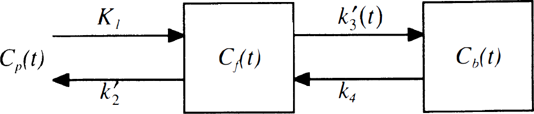
Two-tissue compartmental model to describe neuroreceptor ligand binding. The two compartments represent free and nonspecific tracer (C_f), and specific binding to receptors (C_b). The plasma-tissue exchange constants across the blood—brain barrier are K₁ and k₂', the free plus nonspecific volume of distribution is V_e = K₁/k₂', k₃(t) is the receptor binding rate, and k₄ = k_off is the dissociation rate. Because neurotransmitter competes with tracer for neuroreceptor binding, the tracer binding rate (k'₃(t)) is time-dependent when the neurotransmitter concentration varies with time.

Simulations

To simulate a variety of hypothetical tracers, a range of kinetic parameters was chosen based on the published kinetics of several reversible PET ligands, including [¹¹C]raclopride (Farde et al., 1989), [¹¹C]flumazenil (Koeppe et al., 1991), and [¹⁸F]cyclofoxy (Carson et al., 1993). The range of parameters tested was K₁ = 0.1 to 1.0 mL·min⁻¹·mL⁻¹, V_e, the distribution space of free plus nonspecifically bound tracer or K₁/k₂' K₁/k₂' = 0.3 to 6.0 mL/mL, k_onB_max = 0.1 to 1.0 min⁻¹, and k_off = 0.02 to 0.25 min⁻¹. Neurotransmitter pulses were modeled as monoexponential curves [N_f(t) = Hexp(−Rt)] with the peak of N_f(t), H = 0.5 K_D^N to 2 K_D^N, is the neurotransmitter affinity and the clearance rate of N_f(t), R = 0.04 to 0.1 min⁻¹. These values for H and R are based on values obtained for amphetamine-induced dopamine pulses in rhesus monkeys, as measured with microdialysis (Endres et al., 1997). From simulations that accompanied those studies, we calculated that baseline dopamine levels had little effect on measured changes in the specific binding of [¹¹C]raclopride. Thus, in these simulations, baseline neurotransmitter level, and hence baseline receptor occupancy, was assumed to be zero. Overall, three to seven values of each parameter were chosen as follows: K₁: 0.1, 0.2, 0.5, 1.0 mL·min⁻¹·mL⁻¹; V_e: 0.3, 0.6, 1.0, 3.0, 6.0 mL/mL; k_onB_max: 0.1, 0.2, 0.5, 1.0 min⁻¹; k_off: 0.02, 0.04, 0.06, 0.08, 0.1, 0.15, 0.25 min⁻¹; H: 0.5 K_D^N, K_D^N, 2 K_D^N nmol/L; R: 0.04, 0.06, 0.1 min⁻¹. Time-activity curves were simulated using all possible parameter combinations. This generated 560 simulated tracers, 9 simulated neurotransmitter pulses, and more than 5,000 simulated curves for both the bolus and B/I methods. To better characterize the relation between neurotransmitter release and the radioligand measurements, select tracers were tested with a larger range of neurotransmitter pulses: H = 0.375 K_D^N to 2.5 K_D^N, and R = 0.03 to 0.15 min⁻¹. The selected tracers included those at the extremes of the simulated range (i.e., tracers having various combinations of the smallest or largest values of k'₂, f₂k_onB_max, and k_off). All simulations were performed without addition of noise. Preliminary simulations showed that including a 4% blood volume had negligible effect on the results; consequently, intravascular radioactivity was ignored.

Bolus method

With bolus tracer delivery, two separate studies are performed to measure neurotransmitter competition (Logan et al., 1991). One study is a control, during which the neurotransmitter concentration is assumed to be constant. The second study includes a stimulus (e.g., amphetamine) that induces neurotransmitter release. In experiments with the bolus method, the total volume of distribution (V) is measured for each study, and the percent change in specific binding (i.e., binding potential) between the control and stimulus studies is calculated to quantitate the effect of the neurotransmitter pulse. However, it is important to recognize that the fraction of V contributed by specific binding will vary across different tracers. For example, a tracer may give a large absolute change in specific binding that corresponds to a small change in the V. Therefore, in this simulation study, from signal-to-noise considerations, the percent change in V will be used as a measure of changes in neurotransmitter concentration (see Discussion).

Simulations of the bolus method were performed using a smoothed metabolite-corrected [¹¹C]raclopride plasma input function from a rhesus monkey. Tissue time-activity curves (C_i(t) were generated from the extended two-compartment model without noise using a fourth-order Runge-Kutta algorithm (Press et al., 1992) with a step size of 0.025 minute for 120 minutes, and larger (up to 1 minute) step sizes thereafter. To simulate PET studies, mean values of the time-activity curves were calculated for a scan protocol of 6 × 30 seconds, 3 × 60 seconds, 2 × 120 seconds, 4 × 300 seconds, 8 × 150 seconds, 10 × 300 seconds, 2 × 600 seconds, for a total scan duration of 120 minutes. For each hypothetical tracer (i.e., each combination of K₁, V_e, k_onB_max, and k_off), a control curve (i.e., with N_f(t) = 0) was generated in addition to the stimulus curves [N_f(t) = Hexp(−Rt)]. For the stimulus curves, the neurotransmitter pulse was initiated coincident with the bolus injection (see Discussion). The effect of the neurotransmitter pulse was assessed by computing the percent reduction in V between the stimulus study and the control study.

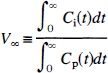
The following methods were used for calculation of V with the bolus method: (1) The slope as measured by Logan graphical analysis with plasma input computed using data from 20 to 60 minutes after injection (V_L¹⁰⁰). (2) Because graphical analysis requires sufficient time to measure an accurate slope, data from 60 to 100 minutes (V_L¹⁰⁰) were used to determine whether the slope measured at a later time would differ from the result obtained in method (1). (3) A one-compartment, two-parameter (K₁, k₂“) model (Koeppe et al., 1991) was fit (unweighted) to 120 minutes of data, and the distribution volume (V₁) was estimated from K₁/k″₂. (4) A two-compartment, four-parameter (K₁, k₂', k₃', k₄) model was fit (unweighted) to 120 minutes of data, and the distribution volume (V₂) was estimated from K₁/k₂'(1 + k₃'/k₄). (5) The ratio of the tissue and plasma integrals (V_∞) was calculated as follows (Lassen and Perl, 1979):

V_{\infty} = \frac{\int_{0}^{\infty} C_{i} (t) d t}{\int_{0}^{\infty} C_{p} (t) d t},

(1)

Methods (1) through (4) used the simulated PET time-activity curves, with the time frames chosen to correspond to the duration of a study with a ¹¹C or ¹⁸F-labeled tracer. To ensure accurate calculation of equation 1, tissue time-activity curves were simulated for an extended duration (more than 10,000 minutes). To perform this calculation, the input function from 5 to 90 minutes was fit to a sum of three exponentials, and then extrapolated. The percent change in the total distribution volume (ΔV) between control and stimulus studies was estimated using each method.

It is not clear a priori whether methods (1) through (5) would give similar estimates of the distribution volume, because the presence of a time-varying neurotransmitter pulse causes the distribution volume (V(t)) to be time-dependent. Therefore, in the stimulus study, the measured distribution volume cannot be interpreted as a fixed value. Theoretical relations between the measured distribution volumes and V(t) are derived in the discussion and appendices. To determine the consistency of the distribution volume estimates between methods, the percent difference and correlation of V and ΔV were determined for each pair of methods using the simulation data.

Bolus-plus-infusion method

Bolus-plus-infusion tracer delivery is used to achieve equilibrium in plasma and tissue (Carson et al., 1993). After equilibrium is attained, a change in neurotransmitter level produces a change in tissue tracer concentration. An advantage of the B/I method over the bolus method is that the effect of a neurotransmitter pulse can be determined in a single study.

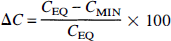
For simulations of the B/I method, it was assumed that tracer equilibrium in plasma and all brain regions was initially achieved. The input function C^p was assumed to be constant throughout the study, and the initial tissue activity was set to the equilibrium level C_EQ, where C_EQ = (K¹/k'₂) · (1 + f₂k_onB_max/k_off)C_p. Then, using the monoexponential neurotransmitter pulse and the differential equations of the extended model, the free and bound tracer concentrations were simulated. The neurotransmitter pulse was initiated, causing the tracer concentration to decrease, achieve a minimum value (C_MIN), then increase toward the original equilibrium level (Fig. 2). Because the minimum concentration corresponds to dC_i/dt = 0, then, from the model differential equations, at that time C_f = (K₁/k'₂)C_p, i.e., the free plus nonspecific concentration is identical to that during the initial equilibrium level, if C_p and K₁/k'₂ are unchanged. Therefore, the change from the initial concentration to the minimum concentration is entirely because of a change in specific binding. For this reason, the maximum percent reduction in tissue concentration (ΔC) was used to evaluate the effect of the neurotransmitter pulse, i.e.,

Δ C \frac{C_{E Q} - C_{M I N}}{C_{E Q}} \times 100

(2)

Note that ΔC is the percent change in the total tissue concentration, as opposed to the percent change in specific binding that is typically measured in PET or SPECT studies. This is analogous to using the total distribution volume in bolus studies (see Discussion).

FIG. 2.

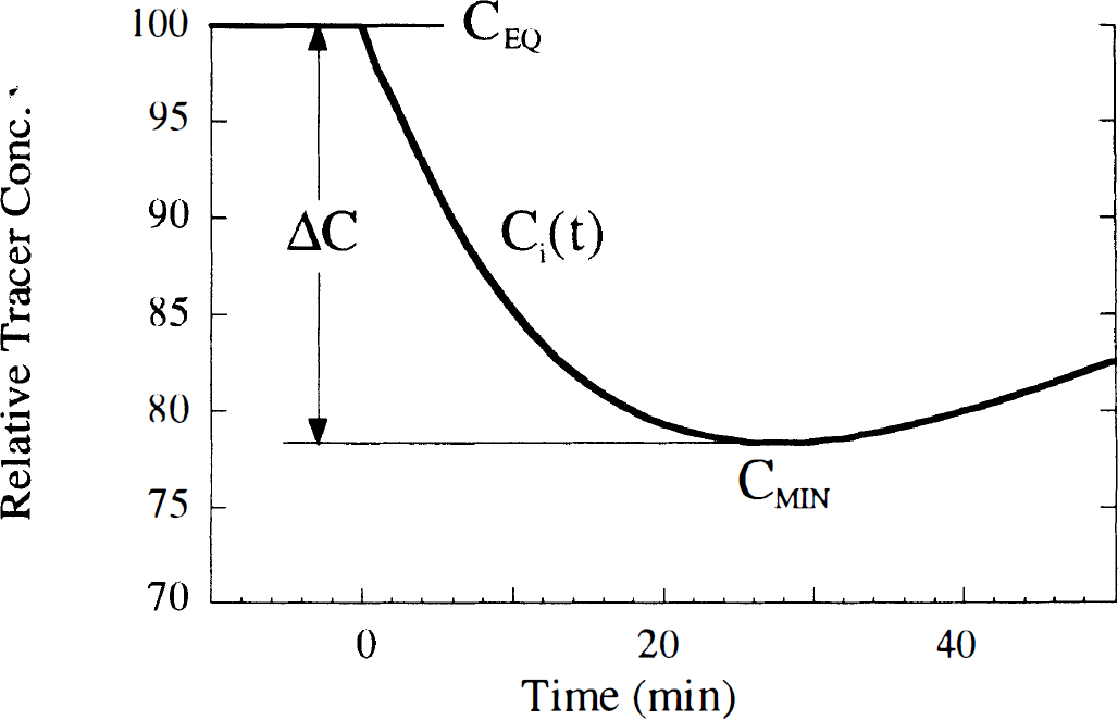
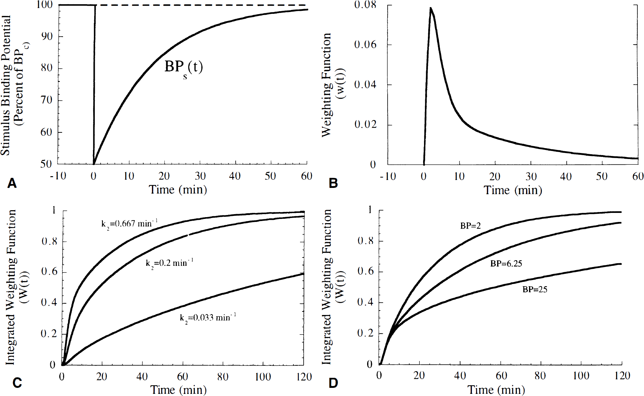
Typical tissue time-activity curve simulated with the bolus-plus-infusion method. The initial concentration of the simulation was set to the equilibrium level C_EQ, where C_EQ = V_e (1 + f₂k_onB_max/k_off)C_p. C_p is the plasma level at equilibrium, k_on is the bimolecular association rate, B_max is the total receptor density, V_e = K₁/k'₂ is the free plus nonspecific volume of distribution, and k_off is the dissociation rate. After equilibrium, a neurotransmitter pulse was initiated causing the tracer concentration to decrease, achieve a minimum value (C_MIN), then increase toward the original equilibrium level. The sensitivity to the neurotransmitter pulse was computed from the maximum percent reduction in concentration (ΔC), where ΔC = 100 × (1 – C_MIN/C_EQ.

Analysis

It was previously shown that the extended model predicts that a change in specific [¹¹C]raclopride binding, measured with the B/I protocol, is proportional to the integral of the dopamine pulse normalized by the neurotransmitter affinity (∫N_f(t)/K_D^N) (Endres et al., 1997). Normalization by K_D^N is necessary because the model is only sensitive to the ratio of free neurotransmitter to its affinity. To determine whether this interpretation is appropriate for other tracers and for both the bolus and B/I methods, we initially tested for linear correlation between ΔV or ΔC and (∫N_f(t)/K_D^N). However, the simulations showed that these relationships often became nonlinear as the neurotransmitter pulse became large because of saturation effects. Therefore, the Spearman rank correlation, which does not assume a particular functional form, was used to determine whether a monotonic relation exists between ΔV or ΔC and ∫N_f(t)/K_D^N. For initial testing of the correlation, N_f(t) was integrated for 40 minutes on the basis of our previous results with [¹¹C]raclopride (Endres et al., 1997). To determine the effect of the integration interval of ∫N_f(t) on the correlation between ΔV or ΔC and ∫N_f(t)/K_D^N, N_f(t) was also integrated for times of 10, 20, 30, 60, 80, and 100 minutes. The correlations of ΔV and ΔC with H and R were also tested.

The simulations were examined to determine how tissue-to-blood transport, receptor density, receptor dissociation rate, binding potential, and nonspecific binding affected the magnitude of ΔV and ΔC, i.e., the sensitivity to neurotransmitter release. Note that we have defined the binding potential as k'₃/k₄ = f₂k_onB_max/k_off, i.e., the equilibrium ratio of bound to free plus nonspecifically bound tracer. Because the parameter K₁ scales the entire time-activity curve, it also scales the estimate of C_i and V. Consequently, varying the value of K₁ did not affect the calculation of percent changes ΔV and ΔC. Therefore, the sensitivity to a neurotransmitter pulse can be characterized in terms of k₂, f₂, k_onB_max, and k_off. To determine the relation between ΔV or ΔC and tissue-to-blood transport, the effect of changing k₂ was examined with the remaining parameters held fixed. The relation with receptor density was studied by varying k_onB_max, and the relation with receptor dissociation rate or binding potential was evaluated by varying k_off. To test the relation with nonspecific binding, we examined the effect of changing f₂ so that k'₂(f₂k₂) and k'₃(f₂k₃) were varied with k'₃/k'₂ held unchanged.

RESULTS

Bolus studies

Estimation of V and ΔV. Table 1 shows the mean and SD of the percent differences in the distribution volume estimates calculated by the five different methods. The small mean values of the percent differences (<2%) for all measures except the one-compartment fit (V₁) indicate that equation 1 (V_∞), the Logan slope (V_L⁶⁰, V_L¹⁰⁰), and the two-compartment fit (V₂) give similar estimates of V even in the presence of a neurotransmitter pulse. From examination of the standard deviations of the percent differences, it is seen that in comparison to the “early” Logan slope (V_L⁶⁰), the “late” Logan slope (V_L¹⁰⁰) was in better agreement with both V₂ and V_∞. This result is supported theoretically, because it can be shown that the Logan slope measured at an increasingly late time converges to V_∞ (see Discussion). Further examination of the percent differences in V revealed that all estimates were in better agreement with each other as k_off increased. For example, the mean ± SD of the percent differences between V₂ and V_∞ was 3.0% ± 1.2% with k_off = 0.02 min⁻¹, but only −0.1% ± 0.5% with k_off = 0.25 min⁻¹. The mean ± SD of the percent differences between V_L⁶⁰ and V_L¹⁰⁰ was 0.5% ± 9.1% for k_off = 0.02 min⁻¹, and −0.8% ± 2.7% for k_off = 0.25 min⁻¹. The smaller standard deviation for k_off = 0.25 min⁻¹, indicates that the estimates given by V⁶⁰_L and V¹⁰⁰_L are more consistent at the faster dissociation rate. This suggests that for tracers with rapid dissociation rates, a shorter scan time is sufficient for quantification of the graphical analysis slope. Inspection of the effects of k₂ and k_onB_max did not reveal a pattern in the percent differences of the estimates. The one-compartment fit estimate (V₁) was the least consistent with the other methods, with a mean percent difference more than or equal to 5.1% and large SD. Apparently, in many cases the one-compartment model is not an adequate approximation to the extended model used to generate the data.

TABLE 1.

Percent differences of distribution volume (V) estimated by different methods

	V¹⁰⁰_L	V₂	V⁶⁰_L	V₁
V_∞	0.4 ±	1.3 ± 7.9	0.0 ± 12.5	–5.1 ± 12.1
V¹⁰⁰_L		0.9 ±4.8	−0.4 ± 9.8	−5.5 ±13.1
V₂			−1.3 ± 6.9	−6.4 ±16.5
V_L⁶⁰				–5.1 ± 16.7

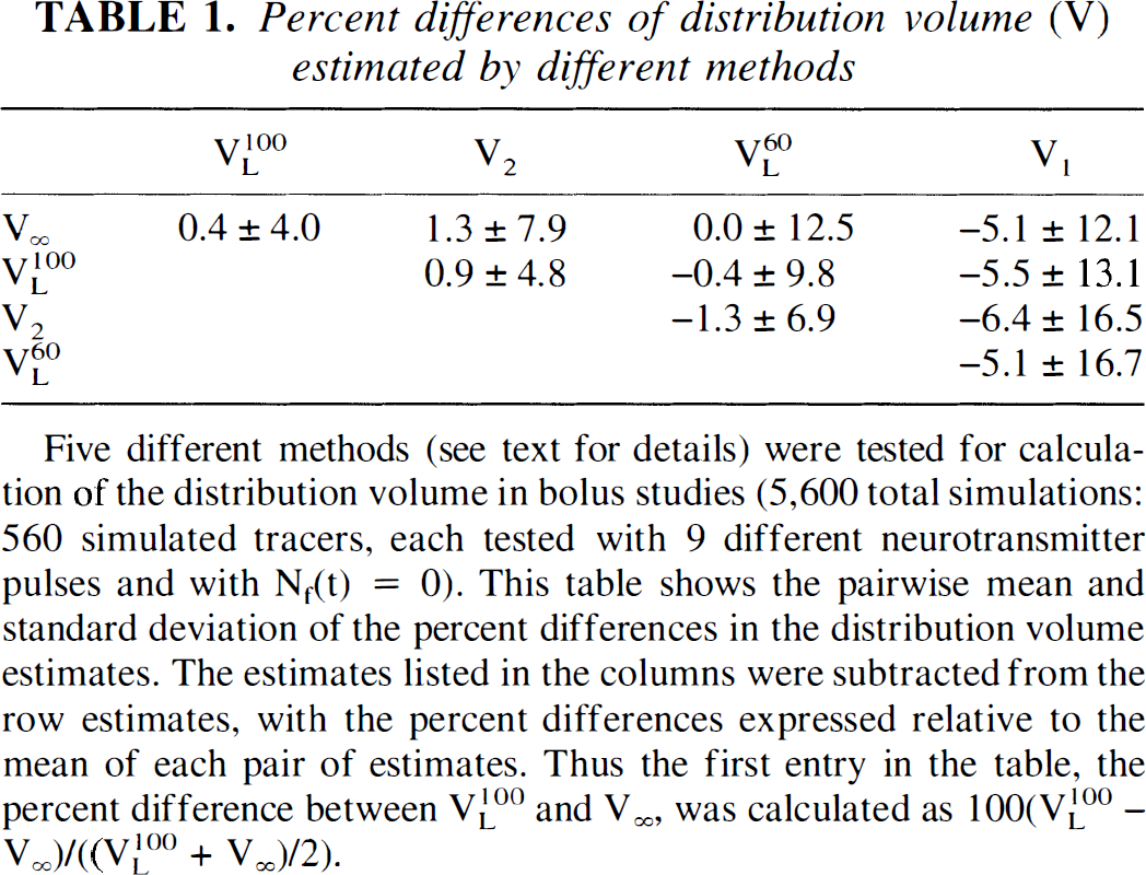
Five different methods (see text for details) were tested for calculation of the distribution volume in bolus studies (5,600 total simulations: 560 simulated tracers, each tested with 9 different neurotransmitter pulses and with N_f(t) = 0). This table shows the pairwise mean and standard deviation of the percent differences in the distribution volume estimates. The estimates listed in the columns were subtracted from the row estimates, with the percent differences expressed relative to the mean of each pair of estimates. Thus the first entry in the table, the percent difference between V¹⁰⁰_L and V_∞, was calculated as 100(V¹⁰⁰_L – V_∞)/((V_L¹⁰⁰ + V_∞)/2).

Table 2 shows the relationship between ΔV values estimated by the different methods. The mean percent differences of the ΔV values estimated by V_∞, V_L¹⁰⁰, and V₂ are small (<3%), with very high linear correlation coefficients (r > 0.97). In particular, the estimates of ΔV given by V_∞ and V_L¹⁰⁰ were practically identical (r = .998, mean ± SD = −0.6% ± 2.0%). These results suggest that V_∞, V_L¹⁰⁰, or V2 would provide very similar quantification of these studies. Because it is more commonly used, ΔV as measured by Logan graphical analysis (V_L¹⁰⁰) was used for further evaluation of the simulation results.

TABLE 2.

Percent difference and correlations of ΔV estimated by different methods

	V_L¹⁰⁰	V₂	V_L⁶⁰	V₁
Percent difference
V_∞	−0.6 ± 2,0%	−2,3 ± 7,2%	0,6± 12,7%	14.2±20,2%
V¹⁰⁰_L		–1.7 ± 5,8%	1.2 ± 11.1%	14,7±20,2%
V₂			2.9 ± 10.0%	16.4 ± 21.6%
V⁶⁰_L				13.6 ±21.3%
Correlations
V_∞	.998	.976	.923	.874
V_L¹⁰⁰		.985	.942	.876
V₂			.955	.851
V_L⁶⁰				.843

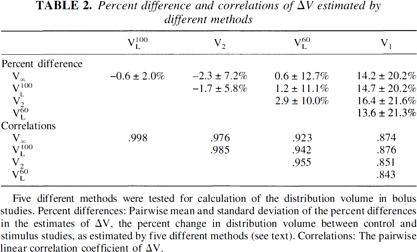
Five different methods were tested for calculation of the distribution volume in bolus studies. Percent differences: Pairwise mean and standard deviation of the percent differences in the estimates of ΔV, the percent change in distribution volume between control and stimulus studies, as estimated by five different methods (see text). Correlations: The pairwise linear correlation coefficient of ΔV.

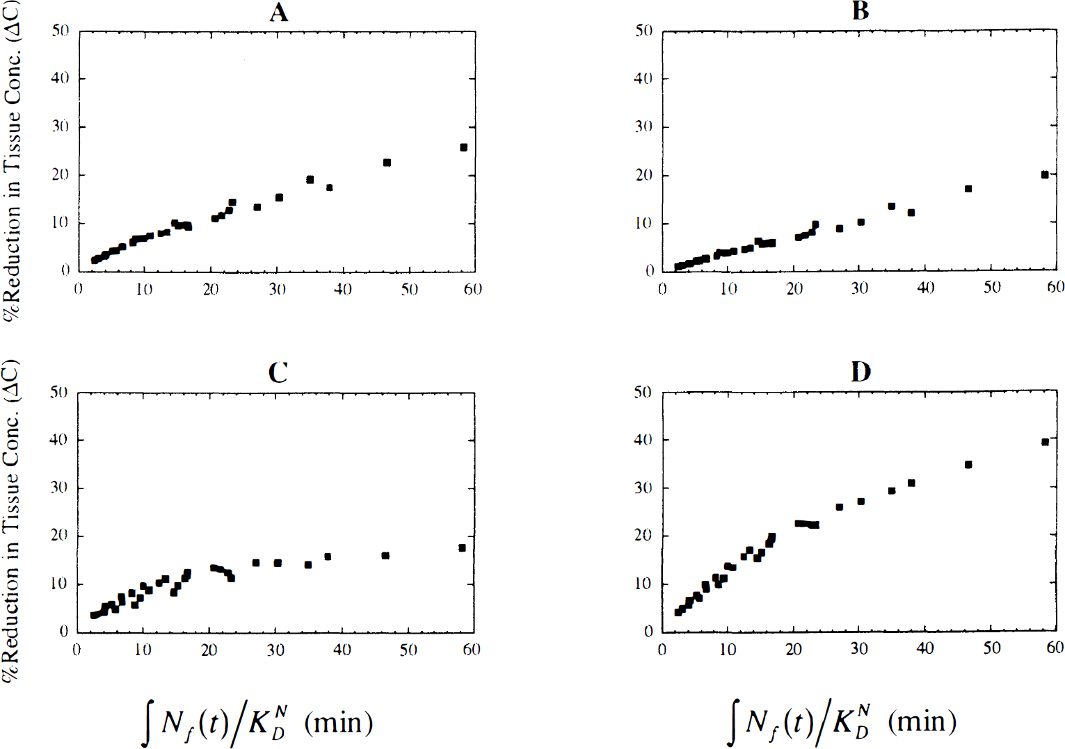
Relation between ΔV and the integrated neurotransmitter pulse. Figure 3 shows examples of the relationship between ΔV and the integrated neurotransmitter pulse (∫N_f(t)/K_D^N, with N_f(t) integrated for 40 minutes) for four tracers with different kinetics. Across all the simulated tracers (n = 560), the linear correlation between ΔV and ∫N_f(t)/K_D^N was 0.93 ± 0.08. For more than 80% of the tracers, the linear correlation was greater than 0.9. However, for tracers with very slow clearance rates (e.g., k'₂ = 0.0166 min⁻¹, f₂k_onB_max = 1.0 min⁻¹, and k_off = 0.02 min⁻¹), the correlation was smaller, with the lowest value being r = 0.64.

FIG. 3.

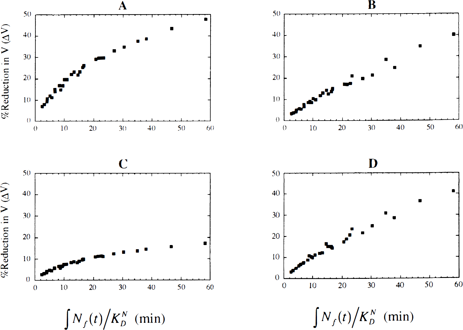
The percent reduction in distribution volume (ΔV) between control and stimulus studies versus the normalized integral of the free neurotransmitter concentration (∫N_f(t)/K^N_D) for four different tracers. To calculate ∫N_f(t)/K^N_D, N_f(t) was integrated from 0 to 40 minutes. The graphical analysis slope (V¹⁰⁰_L) was used to calculate ΔV. All results were independent of K₁. Tracer kinetics are as follows: (A) k'₂ = 0.333 min⁻¹; f₂k_onB_max = 0.1 min⁻¹, k_off = 0.02 min⁻¹; (B) k'₂ = 0.333 min⁻¹, f₂k_onB_max = 1.0 min⁻¹, k_off = 0.02 min⁻¹; (C) k'₂ = 0.333 min⁻¹, f₂k_onB_max = 0.1 min⁻¹, k_off = 0.25 min⁻¹; and (D) k'₂ = 0.167 min⁻¹, f₂k_onB_max = 1.0 min⁻¹, k_off = 0.25 min⁻¹. Neurotransmitter pulses (N_f(t) = Hexp(−Rt)) were generated with H = 0.375 K^N_D, 0.625 K^N_D, K^N_D, 1.5 K^N_D, 2 K^N_D, and 2.5 K^N_D; and R = .03, .06, .09, 0.12, and 0.15 min⁻¹ for a total of 30 simulated pulses.

In general, the relation between ΔV and ∫N_f(t)/K_D^N did not remain linear for large pulses because of receptor saturation effects (Fig. 3). Therefore, linear correlation may not be appropriate for characterization of the relation between ΔV and ∫N_f(t)/K_D^N. Therefore, we calculated the Spearman rank correlation, which does not depend on an assumed functional form. The Spearman correlation gave similar results to the linear correlation, i.e., r greater than 0.9, except for tracers with very slow clearance rates. This indicates that for any tracer with kinetics within the range tested here, the larger the integral of the neurotransmitter pulse, the larger the ΔV. Integration of N_f(t) for longer than 40 minutes (up to 100 minutes) had little effect on the correlation. In general, the correlation of ΔV with either H or R was much smaller than the correlation of ΔV with ∫N_f(t)/K_D^N. For tracers with large k₂, the correlation of ΔV with H was as large as 0.91; however, this was still smaller than the correlation between ΔV and ∫N_f(t)/K_D^N.

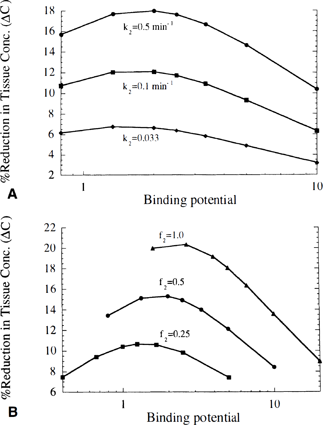
Effect of tracer kinetic characteristics on ΔV. Figure 4 shows ΔV for a range of k_onB_max and k_off values, plotted as a function of k_onB_max (Fig. 4A), k_off (Fig. 4B), and binding potential (Fig. 4C). For a given k_off, ΔV was maximized at a particular value of k_onB_max (Fig. 4A), i.e., the tracer is maximally sensitive to neurotransmitter changes at a particular receptor density. Alternatively, for a fixed value of k_onB_max, ΔV is maximized with a tracer having a particular dissociation rate (Fig. 4B). For small k_onB_max (e.g., low receptor density), a tracer with small k_off (slow dissociation) gave the best contrast (largest ΔV), whereas a larger k_off value provided best contrast when k_onB_max was large. Thus, tracers giving good contrast had similar binding potentials (Fig. 4C). Therefore, the binding potential appeared to be a more useful parameter than either k_onB_max or k_off to characterize the sensitivity of a tracer to neurotransmitter changes, and was subsequently used to describe the simulation results. Note that in many cases, a wide range of binding potential values produced very similar ΔV values. Figure 4C also shows that at a given binding potential, a tracer with low receptor density (and therefore, small k_off) will yield a slightly larger ΔV than a tracer with a high receptor density (large k_off). However, this effect is smaller when k₂ is large, in which case tracers with similar binding potential yield nearly identical ΔV values.

FIG. 4.

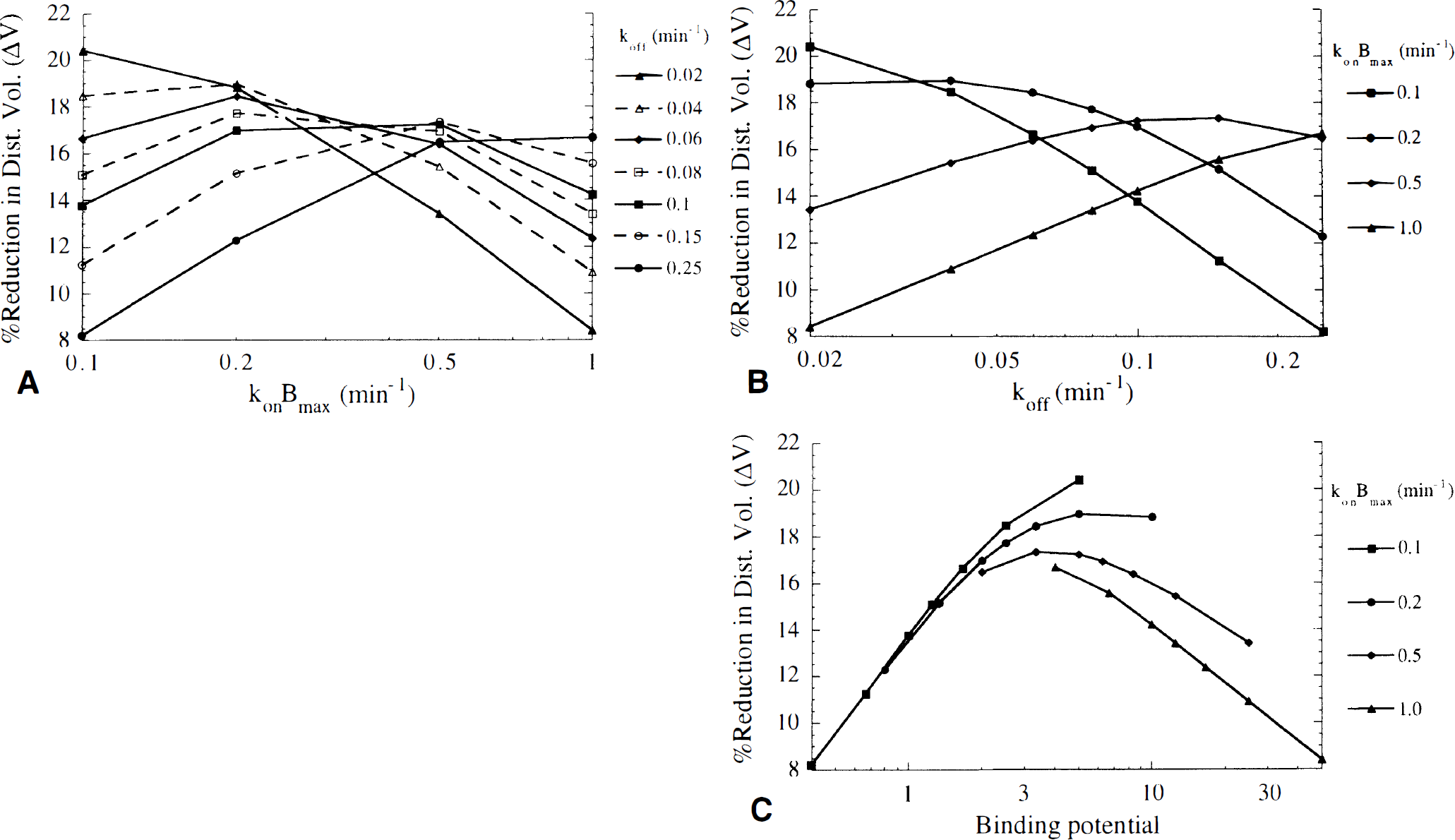
Profile of the percent reduction in distribution volume (ΔV) versus k_onB_max (A); k_off (B); binding potential = f₂k_onB_max/k_off (C). Studies with bolus tracer injection were simulated with N_f(t) = K^N_Dexp(−0.06t), k'₂ = 1.0 min⁻¹, k_off = 0.02 to 0.25 min⁻¹, and f₂k_onB_max = 0.1 to 1.0 min⁻¹. The same data are shown in each plot. Figures 4A and B show considerable scatter, whereas Fig. 4C shows that ΔV is maximized at a similar binding potential.

Figure 5 shows the effects of tissue clearance (k₂, Fig. 5A), and nonspecific binding (f₂, Fig. 5B) on ΔV. The value of ΔV increased as k₂ increased. In addition, the optimal binding potential was larger as k₂ increased. For example, with k₂ = 0.1 min⁻¹, ΔV was largest for binding potentials of ~ 3 to 6, but with k₂ = 0.5 min⁻¹, ΔV was largest for binding potentials of ~5 to 10. However, in most cases ΔV decreased slowly as the binding potential diverged from the optimum value. Thus with k₂ = 0.5 min⁻¹, binding potentials from ~2 to 25 provided contrast within 15% of the maximum ΔV value. Figure 5B shows that ΔV decreased as nonspecific binding increased, i.e., as f₂ decreased. Thus, rapid tissue-to-blood clearance, low nonspecific binding, and an appropriate binding potential are desired for a tracer to be maximally sensitive to changes in neurotransmitter concentration when using the bolus method.

FIG. 5.

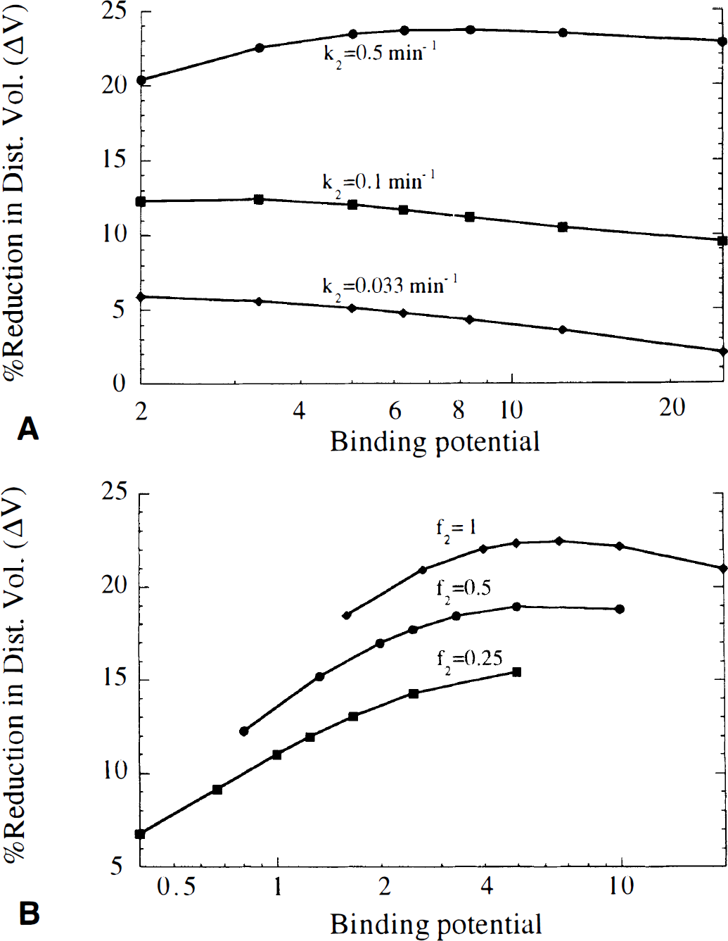
Effects on the percent reduction in distribution volume (ΔV) of (A) tissue-to-blood clearance (k₂), and (B) nonspecific binding (f₂). Bolus studies were simulated with N_f(t) = K^N_Dexp(−0.06t) and k_off= 0.02 to 0.25 min⁻¹. In Fig. 5A, f₂ = 1 and k_onB_max = 0.5 min⁻¹ In Fig. 5B, k_onB_max = 0.4 min⁻¹ and k₂ = 0.4 min⁻¹. Faster tissue-to-blood clearance and less nonspecific binding produce higher ΔV.

Bolus-plus-infusion

Relation between ΔC and the integrated neurotransmitter pulse. Figure 6 shows examples of the relation between the maximum change in tracer concentration (ΔC) from B/I studies and ∫N_f(t)/K^N_D (with N_f(t) integrated for 40 minutes), for four tracers with different kinetics. The linear correlation between ΔC and ∫N_f(t)/K^N_D was very strong for all 560 simulated tracers (r = 0.96 ± 0.04). As was found for ΔV, ΔC usually does not increase linearly at the highest values of ∫N_f(t)/K^N_D because of saturation effects. Therefore, the Spearman rank correlation was calculated, which showed excellent correlation between ΔC and ∫N_f(t)/K^N_D (r ≥ 0.95) for all tracers. The correlation value was somewhat dependent on the integration interval, although the effect was minor. However, it is interesting to note that the integration interval that gave the highest correlation corresponded to the time at which tracer concentration reached its minimum value (C_MIN, Fig. 2). Thus for tracers that were rapidly displaced, ΔC showed higher correlation with the 20-minute integral of N_f(t than it did with the 80-minute integral.

FIG. 6.

The percent reduction in tissue concentration (ΔC) for B/l studies versus ∫N_f(t)/K^N_D for four different tracers. Tracer kinetics and pulse simulations are the same as in the corresponding plots in Fig. 3. The relation is nonlinear for large ∫N_f(t) because of saturation effects.

This could be expected, because after the minimum tracer concentration has been reached, the subsequent neurotransmitter concentration does not influence the measurement of ΔC. Despite this effect, the Spearman correlation was always large (i.e., r ≥ 0.92 for integration intervals from 20 to 80 minutes). Therefore, for any tracer with kinetics in the range tested here, a larger change in tracer concentration (ΔC) can be interpreted as a larger neurotransmitter pulse integral, and this interpretation is not sensitive to the integration interval. For all other tracers tested, ΔC showed better correlation with ∫N_f(t)/K^N_D than H or R, as was previously reported for [¹¹C]raclopride kinetics (Endres et al., 1997). When both k₂ and k_off were large, the correlation of ΔC with H was as large as the correlation of ΔC with ∫N_f(t)/K^N_D.

Effects of tracer kinetic characteristics on ΔC. Figure 7 shows three simulated B/I curves for tracers that have identical kinetics except for different values of k_off, giving binding potentials (BP = f₂k_onB_max/k_off) of 0.8, 3, and 10. The dotted curve (k_off = 0.25, BP = 0.8) shows that when the receptor dissociation rate is fast, the tracer closely follows the transient neurotransmitter pulse and returns quickly to its initial concentration after clearance of neurotransmitter. At a slower dissociation rate (k_off = 0.067, BP = 3, dashed curve), the tracer is displaced more slowly but gives a larger ΔC because of the larger specific binding fraction (75% at BP = 3 versus 44% at BP = 0.8). At an even slower dissociation rate (k_off = 0.02, BP = 10, solid curve), tracer is displaced very slowly, and reaches a minimum concentration at a later time when much of the neurotransmitter has already cleared. Thus, although this tracer has the highest specific binding fraction (91%), it does not show the highest fractional displacement.

FIG. 7.

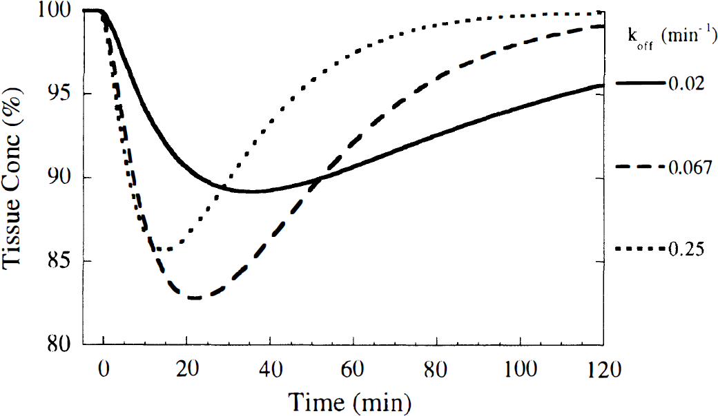
Simulated time course in B/l studies expressed as percent of equilibrium value for three tracers with different rates of receptor dissociation (k_off). These time-activity curves were simulated with N_f(t) = K^N_Dexp(−0.06t), K'₂ = 0.267 min⁻¹, and f₂k_onB_max = 0.2 min⁻¹. The dissociation rates were k_off = 0.02, 0.067, and 0.25 min⁻¹, corresponding to binding potentials (BP) of 10, 3, and 0.8, respectively.

Figure 8 shows the profile of ΔC displayed versus BP. As was found with ΔV (Fig. 4C), the value of ΔC is maximized at a particular value of BP, i.e., the relationship of ΔC and k_onB_max or k_off alone is more scattered as in Figs. 4A and B. Therefore, the BP is a more useful parameter to predict ΔC than either k_onB_max or k_off. However, ΔC was maximized at BP (1 to 2) that were smaller than those that maximized ΔV. This could reflect the importance of rapid dissociation for the B/I method, as larger k_off values correspond to smaller BP. At a given BP, there was a small increase in ΔC for tracers with larger k_onB_max or k_off. Note that this pattern is the reverse of that seen for bolus studies (Fig. 4C). The value of ΔC was increased by faster tissue-to-blood transport (larger k₂) (Fig. 9A), and lower nonspecific binding (higher f₂) (Fig. 9B), in a similar manner to bolus studies (Fig. 5). Unlike bolus studies, the BP that maximized ΔC was not greatly affected by k₂. Across the simulations, BPs of ~0.6 to 4 provided contrast within 15% of the maximum ΔC value.

FIG. 8.

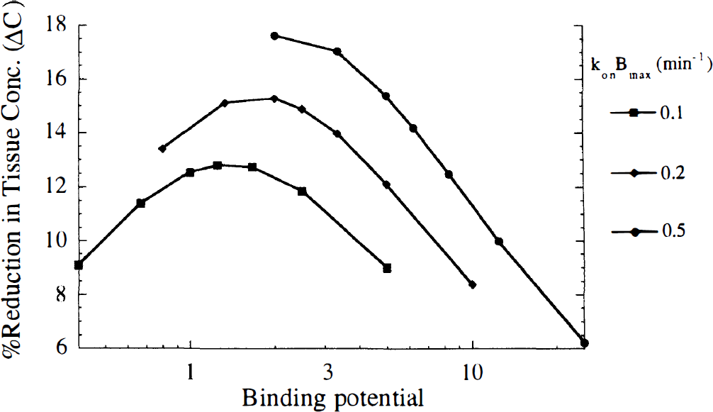
The effect of binding potential on the maximum percent reduction in tissue concentration (ΔC) measured with the B/l method. B/l studies were simulated with N_f(t) = K^N_Dexp(−0.06t), k'₂ = 1.0 min⁻¹, k_off = 0.02 to 0.25 min⁻¹, and f₂k_onB_max = 0.1, 0.2, and 0.5 min⁻¹. Each curve corresponds to a different level of receptor density (k_onB_max). Regardless of the value of k_onB_max, ΔC is maximized at a similar binding potential in an analogous manner to Fig. 4C.

DISCUSSION

Quantification of changes in tracer binding

Neurotransmitter competition studies are typically evaluated by estimating the percent change in specific binding between control and stimulus studies. This requires estimation of the nonspecific fraction, e.g., using a reference tissue region. The percent change in specific binding gives a larger numerical value than ΔV or ΔC, the measures used in these simulations. However, we chose to use ΔV and ΔC to evaluate the sensitivity to a transient neurotransmitter pulse because it is important to include the relative levels of specific and nonspecific binding in judging the suitability of a tracer for these studies. For example, it would be impractical to have a tracer with a specific binding fraction of only 10% of the total concentration even if it had a 50% change in specific binding. In this case, ΔV would only be 5%, indicating that it would be difficult to measure the change in signal. In fact, the simulations revealed that the largest changes in specific binding corresponded to tracers with the smallest BP (data not shown), i.e., tracers with the smallest specific binding fractions. Thus it is misleading to conclude that a tracer is sensitive to changes in neurotransmitter concentration based on a large percent change in specific binding only. The magnitude of ΔV or ΔC is a better predictor of which tracers will yield measurable signals.

Characterizing the bolus method

Methods used for quantification of the distribution volume (e.g., Logan graphical analysis) inherently assume stationarity, i.e., linear time-invariant kinetics. However, with transient neurotransmitter release, the kinetics of a neuroreceptor ligand are nonstationary because of the varying level of receptor occupancy. As a result, the distribution volume V(t) varies with time. To understand the quantification of competition studies using the bolus method, we must determine the relation between the estimated distribution volume and V(t). At any given time, V(t) for the compartment model in Fig. 1 is

V (t) = \frac{K_{1}}{k_{2}^{'}} (1 + \frac{k_{3}^{'} (t)}{k_{4}}) = \frac{K_{1}}{k_{2}^{'}} (1 + \frac{f_{2} B_{max}}{K_{D} (1 + N_{f} (t) / K_{D}^{N})})

(3)

The V_∞ measure (equation 1), can be shown (Appendix A) to be a time-weighted average of V(t), i.e.,

V_{\infty} = \int_{0}^{\infty} w (t) V (t) d t

(4)

where w(t) is a weighting function defined as

w (t) \equiv \frac{C_{f} (t)}{\int_{0}^{\infty} C_{f} (t) d t}

(5)

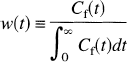
That is, V_∞ is equal to V(t) weighted by the normalized free tracer concentration. This result is similar to that of Huang et al. (1981) for the metabolic rate of glucose measured in fluorodeoxyglucose studies in the presence of a time-varying rate. In that case, the estimated rate is approximately a weighted average of the varying glucose metabolic rate, weighted by the normalized plasma fluorodeoxyglucose concentration, analogous to equations 4 and 5.

Effects of tracer kinetics on measurement of ΔV

The simulations showed that the magnitude of ΔV, i.e., the sensitivity to a change in neurotransmitter concentration, was dependent on kinetic properties of the tracer, including k₂, f₂, k_onB_max, and k_off. To help understand these effects, we use equations 3 and 4 to express ΔV as

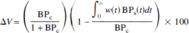
Δ V = (\frac{{B P}_{c}}{1 + {B P}_{c}}) (1 - \frac{\int_{0}^{\infty} w (t) {B P}_{s} (t) d t}{{B P}_{c}}) \times 100

(6)

where BP_c = f₂k_onB_max/k_off, and BP_s(t) = (f₂k_onB_max/k_off)/(1 + N_f<t)/K^N_D) are the binding potentials in the control and stimulus studies, respectively. The first component on the right hand side of equation 6, BP_c/(1 + BP_c), is the specific binding fraction. The second component is the effective percent change in specific binding, and depends on the normalized free tracer concentration, i.e., w(t).

To explain the effects of tracer kinetics on ΔV, we must understand the integral in the second component of equation 6. Consider BP_c and BP_s(t) in a pair of control and stimulus studies (Fig. 10A). Figure 10B shows an example of the weighting function w(t) for a rapidly clearing tracer. From examination of equation 6, ΔV will be larger if the early phase of BP_s(t), when it is most different from BP_c, is weighted more heavily. The sharp peak in w(t) overlaps the initial decrease in BP_s(t), indicating that this tracer should provide good contrast. The largest possible signal could be obtained if w(t) is approximately a delta function coincident with peak saturation. If so, ΔV would correlate best with the peak neurotransmitter concentration, H. However, because w(t) generally has a broad peak, ΔV correlates better with ∫N_f(t) and less so with H.

A useful way to predict the effective percent change in specific binding of different tracers is to display the integral of the weighting function W(t) = ∫^t_ow(τ)dτ. The tracer that gives strongest weight to the initial decrease in BP_s(t) is revealed as the tracer having W(t) reach a maximum value of 1 most quickly. Figure 10C shows W(t) curves for tracers with different tissue-to-blood clearance (k₂) values. For highest k₂ values, W(t) reaches a maximum value of 1 more quickly, consistent with the result that faster k₂ increases ΔV (see Fig. 5A). Figure 10D shows that for larger BP, the integrated weighting function reaches 1 slowly. In this case, the free tracer concentration is prolonged because the specifically bound pool becomes a significant source of free tracer. In other words, for the high BP case, the tracer dissociates slowly from the receptor, but can then rebind to the receptor, which is now unoccupied because the neurotransmitter pulse has substantially cleared.

FIG. 9.

Effects on the maximum percent reduction in tissue concentration (ΔC) of (A) tissue-to-blood clearance (k₂), and (B) nonspecific binding (f₂). B/l studies were simulated with N_f(t) = K^N_Dexp(−0.06t) and k_off = 0.02 to 0.25 min⁻¹. In Fig. 9A, f₂ = 1, and k_onB_max = 0.2 min⁻¹. In Fig. 9B, k₂ = 0.4 min⁻¹, and k_onB_max = 0.4 min⁻¹. The value of ΔC is increased by faster tissue-to-blood transport and less nonspecific binding, similar to the effects seen for ΔV measured with the bolus method (see Fig. 5).

FIG. 10.

(A) The dashed line represents the binding potential (BP_c) in a control study, with a constant neurotransmitter concentration (N_f(t) = 0). The solid curve is the time-varying binding potential (BP_s(t)) in a stimulus study with N_f(t) = K^N_Dexp(−0.06t). (B) An example of the weighting function w(t), (equation 5) as determined from the normalized free tracer concentration. Equation 6 shows that the tracer in Fig. 10B is most sensitive to BP_s(t) when w(t) is large, i.e., in the first 10 minutes. (C) Integrated weighting function, W(t), for tracers with different k₂ values. The tracer that gives strongest weight to the early reduction in BP_s(t) has W(t) reaching a maximum value of 1 most quickly. As tissue-to-blood clearance (k₂) increases, W(t) reaches a maximum value of 1 more quickly, consistent with the result that faster k₂ increases ΔV (see Fig. 5A). (D) W(t) for tracers with different binding potential. Larger binding potential corresponds to slower tracer clearance, which gives suboptimal weighting of BP_s(t). As a result, increasing binding potential does not necessarily increase ΔV (equation 6), even though the specific binding fraction increases.

Therefore, the relation between ΔV and BP can be summarized as a product of the competing effects given by the two components of equation 6. A BP too small leads to small ΔV because of a small specific binding fraction, whereas a BP too large leads to small ΔV because of suboptimal weighting of BP_s(t). This is consistent with the result that ΔV was largest at an intermediate BP (Fig. 4C). This also explains how BP values an order of magnitude apart could give similar ΔV. That is, the competing effects of BP oppose each other such that their product changes slowly as the BP changes.

When the change in specific binding rather than total binding is reported, as is usually done in experiments, the contrast will be greater at smaller BP. This follows the results of Price et al. (1997) that the high affinity D₂ tracer [¹⁸F]fallypride gives less contrast than [¹¹C]raclopride, which has a lower affinity, and therefore, a smaller BP. Similarly, Fowler et al. (1998) showed that the rapidly clearing tracer [¹¹C]cocaine gives larger contrast in measuring dopamine transporter occupancy than the slower clearing [¹¹C]d-threo-methylphenidate.

In these simulations, the monoexponential neurotransmitter pulse was initiated coincident with bolus tracer delivery. Simulations with neurotransmitter release initiated from 1 to 30 minutes earlier or later than tracer delivery gave smaller ΔV (data not shown), in agreement with previous results of Logan et al. (1991). Evidently, simultaneous tracer delivery and neurotransmitter release provides optimal overlap of w(t) and BP_s(t). The drop in ΔV was larger with neurotransmitter release initiated after tracer delivery than with neurotransmitter release initiated before tracer delivery. Therefore, it is better to deliver the stimulus such that neurotransmitter release is induced shortly before arrival of the tracer. This is consistent with the results of Wong et al. (1997) that delivery of amphetamine 5 minutes before [¹¹C]raclopride provides maximum contrast. Similarly, Dewey et al. (1991) reported that an acute dose of amphetamine delivered 2 to 3 minutes before [¹⁸F]-N-methylspiroperidol had a greater effect on tracer binding than amphetamine delivered slowly during a 25-minute period. Another factor affecting the weighting function of equation 5 is the plasma input function. In particular, faster plasma clearance leads to faster tissue clearance, and simulations confirmed that faster plasma clearance causes a more rapid drop in w(t) and increased ΔV values (data not shown).

The weighting function w(t) is derived from the free tracer concentration C_f(t) during the stimulus study. In practice, a control bolus study can be modeled to determine the free tracer profile, which could be used to estimate w(t). This may provide practical insight as to the utility of the tracer for competition studies. A caveat is that the free tracer profile is different in control and stimulus studies because of the effect of neurotransmitter competition on tracer kinetics. In particular, the presence of a neurotransmitter pulse causes free tracer to initially overshoot, then eventually undershoot, the free tracer profile in a control study. Thus the normalized free tracer concentration in a control study predicts lower sensitivity than would actually be expected in a stimulus study.

Simulations performed by Logan et al. (1991) for [¹⁸F]-N-methylspiroperidol indicated that the efflux of tracer from tissue has a significant impact on the sensitivity of in vivo data to endogenous dopamine levels. Even though those simulations dealt with an irreversible tracer, the results agree well with our simulation data of Figs. 5A and 9A, which showed that larger k₂ values enhanced ΔV and ΔC. The theoretical result given by equations 4 and 5, and illustrated in Fig. 10, further clarifies the importance of tracer kinetics, and particularly the free tracer concentration, on the sensitivity to changes in neurotransmitter concentration.

We found that contrast is maximized at a particular value of k_off with slower dissociation rates corresponding to smaller ΔV or ΔC. Thus we concluded that tracers that are nearly irreversible will not provide optimal contrast. This apparently conflicts with the conclusion of Morris et al. (1995) that an irreversible tracer should be most sensitive to changes in dopamine concentration. Their result was determined from using the sum of the squared differences between control and stimulus time-activity curves as a measure for the bolus method, whereas here we used the percent change in the distribution volume. (Note that V cannot be measured for an irreversible tracer.) Thus, for the irreversible case, the sum of squared differences may be a sensitive measure; however, unlike the ΔV measure, such an approach assumes an identical input function for the control and stimulus studies.

Comparison of methods to estimate V

The simulation results showed excellent agreement in the estimates of V and ΔV given by V_∞, V¹⁰⁰_L, and V₂. Thus, V_∞, V¹⁰⁰_L, and V₂ are nearly equivalent even for non stationary kinetics. Furthermore, inspection of the graphical analysis equation revealed that the Logan slope approaches V_∞ with increasing time (see Appendix B). This theoretical result is consistent with the smaller standard deviation in the percent differences between V_∞ and V¹⁰⁰_L (4.0%), compared with that between V_∞ and V⁶⁰_L (12.5%). The similarity of the estimates indicates that as was determined for V_∞, the V¹⁰⁰_L and V₂ measures are approximately weighted averages of V(t), as given by equations 4 and 5. Because these measures all provide very similar quantification of the system, the simplest method can be used to analyze studies. Thus, Logan graphical analysis, which is a simple linear fit and is the most commonly used in practice, is preferred over the other methods tested if V is the only measure of interest. The discrepancy in the V and ΔV estimates given by the one-compartment model (V₁) is not unexpected. Note that even for a stationary system, V₁ would give an inaccurate estimate of V as a result of modeling the tissue kinetics with a single compartment. A single compartment best approximates the system when the receptor dissociation rate is fast. Accordingly, V₁ was in better agreement with the other estimates when k_off values were large.

Characterizing the B/I method

With the B/I method, tracer ideally achieves equilibrium levels in plasma and tissue, which leads to straightforward calculation of V from the tissue-to-plasma ratio. An advantage of the B/I method is that blood sampling is not required in neurotransmitter competition studies, although there are reference region methods appropriate for bolus studies that also do not require blood sampling (Hume et al., 1992; Watabe et al., 1995; Ichise et al., 1996; Lammertsma and Hume, 1996). Here, the initial tissue concentration is used as a reference for measurement of the percent change in concentration (ΔC) caused by neurotransmitter release (equation 2). Typically, several data points are averaged to measure the post-stimulus concentration, although here we used the minimum tissue concentration. As discussed above, V(t) changes continuously after neurotransmitter release; therefore, the minimum concentration does not correspond to a fixed change in V. Because there is no analytical solution to the model differential equations, we cannot derive a theoretical expression for C_MIN or ΔC. However, because ΔC is the change in total concentration, we can consider ΔC to be the product of two effects, in analogy to equation 6. That is, ΔC equals the specific binding fraction times the percent change in specific binding.

For the B/I method, the magnitude of the change in specific binding depends on the ability of the tracer to be displaced from receptors and subsequently cleared from tissue. For example, faster tissue-to-blood clearance leads to greater ΔC (Fig. 9A). The simulation results also showed that the effect of BP on ΔC was similar to the effect on ΔV. This can be explained as a product of competing effects of the BP on ΔC. Consider that a large BP corresponds to a slow receptor dissociation rate, a fast association rate (k_onB_max), or possibly both. These properties cause tracer to clear slowly; therefore, an increase in neurotransmitter concentration induces a smaller decrease in specific binding when the BP is large. This explains why a larger BP will not necessarily give a larger ΔC value even though the specific binding fraction is larger (Fig. 8). This also may explain the results of Laruelle et al. (1997), that [¹²³I]iodobenzofuran, a D₂ tracer with very high affinity (large BP) was less sensitive to changes in dopamine concentration than [¹²³I]iodobenzamide, a tracer with lower affinity. Furthermore, Laruelle et al. (1996) found in human studies that 0.3 mg/kg amphetamine produced an 8% decrease in [¹²³I]iodobenzamide binding, whereas Breier et al. (1997) showed that a smaller amphetamine dose (0.2 mg/kg) produced a larger decrease (15%) in [¹¹C]raclopride binding. This may be because [¹¹C]raclopride has a lower affinity (smaller BP) than [¹²³I]iodobenzamide. That ΔC was maximized at small BP (1 to 2) illustrates that the B/I method is more sensitive when used with lower affinity tracers. In addition, a lower affinity has the advantage that the initial equilibrium level can be established more quickly.

Accuracy of the model

The extended model was originally developed to analyze [¹¹C]raclopride-PET and dopamine-microdialysis data acquired simultaneously (Endres et al., 1997). In the time frame of these experiments (90 minutes), the model was sufficient to describe the time-activity curves. However, the assumptions of the model may not be adequate to fully describe the true in vivo system. For example, in these simulations a monoexponential curve was used to describe the neurotransmitter pulse, based on microdialysis measurements in rhesus monkey (Endres et al., 1997). However, the 10-minute microdialysis sampling interval limited our ability to more accurately define the pulse shape.

In these simulations, we have assumed that the baseline neurotransmitter concentration is negligible. However, if we include a baseline concentration of neurotransmitter, N₀, it can be shown that the simulation equations are unchanged except that the interpretations of B_max and K^N_D are different. In particular, B_max should be interpreted as the initial free receptor concentration B'_max [B_max/(1 + N₀/K^N_D)], and the neurotransmitter affinity K^N_D should be replaced with K^N_D + N₀. Thus, a system with baseline neurotransmitter is mathematically equivalent to a system with zero baseline concentration, but with a smaller receptor density and lower affinity. Therefore, the presence of baseline neurotransmitter may be expected to lower ΔV and ΔC because the neurotransmitter pulse is less potent.

Another factor not included in the model is the presence of multiple receptor affinity states for neurotransmitter binding. In that case, the observed response (ΔV and ΔC) would be a weighted sum of the response of the individual affinity states, in which the weight is the proportion of receptors in each affinity state. Thus with a combination of high and low affinity states, the resulting curves in Figs. 3 and 6 would still show a monotonic relationship with ∫N_f(t), but the shape would be more complicated because it would reflect the weighted sum of two curves. Because the optimal binding potential values for bolus and B/I studies were found to be independent of the pulse size, these values should be unchanged by the presence of multiple affinity states.

In B/I simulations, the model predicts that after clearance of the neurotransmitter pulse, the tracer concentration will eventually return to its initial equilibrium level (Fig. 2). The return to the initial concentration has not been seen in PET studies, possibly because the scan time is too short to observe this effect. However, SPECT studies using much longer scans indicate that the reduction in tracer concentration lasts for several hours (Malison et al., 1995; Laruelle et al., 1997), which is considerably longer than expected. The prolonged reduction may be caused by receptor internalization, or could be an effect of multiple affinity states for neurotransmitter binding (Laruelle et al., 1997). This may indicate that modification of the extended model is likely to be necessary to fully describe neurotransmitter competition.

Signal-to-noise issues

This simulation study was concerned with describing the tissue signal (ΔV or ΔC) in terms of neurotransmitter release and the kinetic characteristics of the tracer. For this purpose, the effect of measurement noise was not considered. However, maximizing ΔV or ΔC is not equivalent to optimizing contrast in a signal-to-noise sense, because there are situations when a smaller signal can be measured more reliably than a larger signal. For example, the simulations showed that faster tissue-to-blood transport (k₂) improves sensitivity. However, faster tissue clearance also reduces tissue radioactivity, which would increase measurement noise. In addition, the half-life of the radioisotope used, the total dose delivered, and the rate of peripheral metabolism and clearance affect the noise properties of a tracer. Thus, the guidelines shown here may be most useful in comparing a class of receptor-binding analogs that differ in affinity or nonspecific binding levels in the tissue, but are labeled with the same isotope and have similar peripheral clearance and metabolism, i.e., the tracers have similar input functions and produce similar image noise levels.

The choice of optimal experimental design, i.e., bolus versus B/I, must be considered carefully. One advantage of the bolus technique is that the entire time-activity curve contributes to the measurement, rather than just a few scans at equilibrium. With the B/I method, there may not be sufficient time to reach equilibrium, which would bias the estimate of ΔC. Advantages of the B/I method are that it only requires a single radiotracer synthesis, and involves a shorter total study duration. In comparison of the measures obtained with each method, the bolus signal (ΔV) was larger than the B/I signal (ΔC) for BP greater than 1. The measures were comparable at smaller BP, with ΔC being slightly larger than ΔV for BP less than 1. Thus for a rapidly reversible tracer such as [¹¹C]raclopride, the simulations predict that ΔV will be larger than ΔC. This agrees with the results of amphetamine-induced changes in the specific binding of [¹¹C]raclopride as measured with both the bolus and B/I methods (Carson et al., 1997). However, the effects of noise and model accuracy need to be considered more fully to determine whether to use the bolus method or the infusion method to study neurotransmitter competition with a particular tracer. Most important is that the simulation results indicate that both the bolus and B/I methods yield measures that are highly correlated with the underlying changes in neurotransmitter concentration.

Footnotes

Acknowledgments

The authors thank Drs. William C. Eckelman, Peter Herscovitch, and Hiroshi Watabe for their helpful comments and suggestions.

Abbreviations used

APPENDIX A

Consider a bolus injection study for a stationary system, i.e., a system with time-invariant kinetics. In such a study, the total volume of distribution (V) is constant and can be calculated in a variety of ways. Classically (Lassen and Perl, 1979), V can be determined by V_∞:

For a bolus study in a non stationary system, the right-hand side of equation A1 can still be calculated, but the result can no longer be interpreted as a fixed distribution volume. In this appendix, we derive the relation between V_∞ and the time-dependent total distribution volume (V(t), equation 3). Inserting C_i = C_f + C_b into equation A1 yields

The integrals of C_f and C_b can be computed by integrating the model differential equations from zero to infinity.

For a bolus injection, the left-hand side of each equation is zero. Solving for the integrals of C_f and C_b and insertion into equation A2 gives

With the definition of V(t) in equation 3, equation A4 can be written as

where w(t) is a weighting function

Thus, V_∞ is equal to the average of V(t) as weighted by the normalized free tracer concentration. This indicates that V_∞ will be more heavily weighted toward the values of V(t) when C_f is at its peak, e.g., near the beginning of a bolus study.

APPENDIX B

The graphical analysis procedure (Logan et al., 1990) generates the equation:

Beyond a certain time, the curve of (∫C_idt/C_i) versus (∫C_pdt/C_i) becomes linear, with intercept I, and with slope V_L, which is an estimate of V. In this appendix, we determine the relation between the distribution volume estimates obtained by equation 1 (V_∞) and equation B1 (V_L). An explicit formula for the instantaneous value of V_L can be derived from V_L = dy/dx, where y = ∫C_idt/C_i and x = ∫C_pdt/C_i.

Dividing by C_i and setting γ(t) = –(dC_i/dt)/C_i (the fractional rate of change of C_i), V_L becomes

In a constant infusion study, when equilibrium is reached, γ(t) = 0, then equation B3 gives V_L(t) = C_i/C_p. In a bolus study, as t → ∞ and C_p and C_i approach zero, equation B3 gives V_L(t) ≅ V_∞ (equation 1). To approximate V_L(t) at earlier times, changing the bounds of integration of equation B3 yields

Consider the case in which the plasma input function can be described by a sum of exponential functions

with 0 < β₁ < β₂ < … < β_n, the tissue impulse response function h(t) is described by

with 0 < α₁ < α₂ < … < α_m, and the tissue function C_i(t) given by

After a derivation in Carson et al. (1993), if the smallest eigenvalue of the impulse response function α₁ is larger than the smallest exponent in the input function β₁, then after sufficient time, transient equilibrium is achieved and the tissue function is approximately

where C₀ is a constant. For C_i(t) in equation B8, γ(t) = –β₁ and it can be shown that the terms in parentheses in equation B4 equal zero, therefore, V_L becomes equivalent to V_∞. If an initially nonstationary system becomes stationary over time, e.g., neuroreceptor binding after clearance of a transient neurotransmitter pulse, then equation B8 will still be valid. Therefore, after a time in which equation B8 is satisfied, V_L provides an estimate that is approximately equal to V_∞.

References

Breier

Saunders

Carson

Kolachana

DeBartolomeis

Weinberger

Weisenfeld

Malhotra

Eckelman

Pickar

(1997) Schizophrenia is associated with elevated amphetamine-induced synaptic dopamine concentrations—evidence from a novel positron emission tomography method. Proc Natl Acad Sci USA 94:2569–2574

Carson

Channing

Blasberg

Dunn

Cohen

Rice

Herscovitch

(1993) Comparison of bolus and infusion methods for receptor quantitation: application to [18F]cyclofoxy and positron emission tomography. J Cereb Blood Flow Metab 13:24–42

Carson

Breier

De Bartolomeis

Saunders

Schmall

Der

Pickar

Eckelman

(1997) Quantification of amphetamine-induced dopamine release with [11C]-raclopride and continuous infusion. J Cereb Blood Flow Metab 17:437–447

Dewey

Logan

Wolf

Brodie

Angrist

Fowler

Volkow

(1991) Amphetamine induced decreases in (18F)-N-methylspiroperidol binding in the baboon brain using positron emission tomography (PET). Synapse 7:324–327

Dewey

Smith

Logan

Alexoff

Ding

King

Pappas

Brodie

Ashby

Jr (1995) Serotonergic modulation of striatal dopamine measured with positron emission tomography (PET) and in vivo microdialysis. J Neurosci 15:821–829

Endres

Kolachana

Saunders

Weinberger

Breier

Eckelman

Carson

(1997) Kinetic modeling of [11C]raclopride: combined PET-microdialysis studies. J Cereb Blood Flow Metab 17:932–942

Farde

Eriksson

Blomquist

Halldin

(1989) Kinetic analysis of central [11C]raclopride binding to D2-dopamine receptors studied by PET—a comparison to the equilibrium analysis. J Cereb Blood Flow Metab 9:696–708

Fowler

Volkow

Logan

Gatley

Pappas

King

Ding

Y-S

Wang

G-J

(1998) Measuring dopamine transporter occupancy by cocaine in vivo: radiotracer considerations. Synapse 28:111–116

Huang

Phelps

Hoffman

Kuhl

(1981) Error sensitivity of fluorodeoxyglucose method for measurement of cerebral metabolic rate of glucose. J Cereb Blood Flow Metab 1:391–401

10.

Hume

Myers

Bloomfield

Opacka-Juffry

Cremer

Ahier

Luthra

Brooks

Lammertsma

(1992) Quantitation of carbon-11-labeled raclopride in rat striatum using positron emission tomography. Synapse 12:47–54

11.

Ichise

Ballinger

Golan

Vines

Luong

Tsai

Kung

(1996) Noninvasive quantification of dopamine D2 receptors with iodine-123-IBF SPECT. J Nucl Med 37:513–520

12.

Innis

Malison

Al-Tikriti

Hoffer

Sybirska

Seibyl

(1992) Amphetamine-stimulated dopamine release competes in vivo for [123I]IBZM binding to the D2 receptor in nonhuman primates. Synapse 10:177–184

13.

Koeppe

Holthoff

Frey

Kilbourn

Kuhl

(1991) Compartmental analysis of [11C]flumazenil kinetics for the estimation of ligand transport rate and receptor distribution using positron emission tomography. J Cereb Blood Flow Metab 11:735–744

14.

Lammertsma

Hume

(1996) Simplified reference tissue model for PET receptor studies. Neuroimage 4: 153–158

15.

Laruelle

Abi-Dargham

Van Dyck

Gil

D'Souza

Erdos

McCance

Rosenblatt

Fingado

Zoghbi

Baldwin

Seibyl

Krystal

Charney

Innis

(1996) Single photon emission computerized tomography imaging of amphetamine-induced dopamine release in drug-free schizophrenic subjects. Proc Natl Acad Sci USA 93:9235–9240

16.

Laruelle

Iyer

Al-Tikriti

Zea-Ponce

Malison

Zoghbi

Baldwin

Kung

Charney

Hoffer

Innis

Bradberry

(1997) Microdialysis and SPECT measurements of amphetamine-induced dopamine release in nonhuman-primates. Synapse 25: 1–14

17.

Lassen

Perl

(1979) Tracer Kinetic Methods in Medical Physiology, New York, Raven Press

18.

Logan

Fowler

Volkow

Wolf

Dewey

Schlyer

MacGregor

Hitzemann

Bendriem

Gatley

Christman

(1990) Graphical analysis of reversible radioligand binding from time-activity measurements applied to [N-'11C-methyl]-(—)-cocaine: PET studies in human subjects. J Cereb Blood Flow Metab 10:740–747

19.

Logan

Dewey

Wolf

Fowler

Brodie

Angrist

Volkow

Gatley

(1991) Effects of endogenous dopamine on measures of [18F]N-methylspiroperidol binding in the basal ganglia: comparison of simulations and experimental results from PET studies in baboons. Synapse 9:195–207

20.

Malison

Best

Wallace

McCance

Laruelle

Zoghbi

(1995) Euphorigenic doses of cocaine reduce [123I]beta-CIT SPECT measures of dopamine transporter availability in human cocaine addicts. Psychopharmacology (Berl) 122:358–362

21.

Mintun

Raichle

Kilbourn

Wooten

Welch

(1984) A quantitative model for the in vivo assessment of drug binding sites with positron emission tomography. Ann Neurol 15:217–227

22.

Morris

Fisher

Alpert

Rauch

Fischman

(1995) In-vivo imaging of neuromodulation using positron emission tomography—optimal ligand characteristics and task length for detection of activation. Hum Brain Map 3:35–55

23.

Press

Teukolsky

Vetterling

Flannery

(1992) Numerical Recipes in C: The Art of Scientific Computing, 2nd ed, Cambridge, Cambridge University Press

24.

Price

Mason

Lopresti

Holt

Simpson

Drevets

Smith

Mathis

(1997) PET measurement of endogenous neurotransmitter activity using high and low affinity radiotracers. Neuroimage 5:B77

25.

Volkow

Wang

Fowler

Logan

Schlyer

Hitzemann

(1994) Imaging endogenous dopamine competition with [11C]raclopride in the human brain. Synapse 16:255–262

26.

Watabe

Hatazawa

Ishiwata

Ido

Itoh

Iwata

Takahashi

Hatano

Nakamura

(1995) Linearized method: a new approach for kinetic analysis of central dopamine D2 receptor specific binding. IEEE Trans Med Imag 14:688–696

27.

Wong

Yokoi

Hong

Grunder

Szymanski

Nestadt

Neufeld

Schlaepfer

Pearlson

Gjedde

(1997) Quantification of extracellular dopamine release in schizophrenia and cocaine use. Neuroimage 5:B78

Assessment of Dynamic Neurotransmitter Changes with Bolus or Infusion Delivery of Neuroreceptor Ligands

Abstract

Keywords

METHODS

Study overview

Simulations

Bolus method

Bolus-plus-infusion method

Analysis

RESULTS

Bolus studies

Bolus-plus-infusion

DISCUSSION

Quantification of changes in tracer binding

Characterizing the bolus method

Effects of tracer kinetics on measurement of ΔV

Comparison of methods to estimate V

Characterizing the B/I method

Accuracy of the model

Signal-to-noise issues

Footnotes

Acknowledgments

Abbreviations used

APPENDIX A

APPENDIX B

References