Sage Journals: Discover world-class research

Abstract

The authors determined cerebral blood flow (CBF) with magnetic resonance imaging (MRI) of contrast agent bolus passage and compared the results with those obtained by O-15 labeled water (H₂¹⁵O) and positron emission tomography (PET). Six pigs were examined by MRI and PET under normo- and hypercapnic conditions. After dose normalization and introduction of an empirical constant Φ_Gd, absolute regional CBF was calculated from MRI. The spatial resolution and the signal-to-noise ratio of CBF measurements by MRI were better than by the H₂¹⁵O-PET protocol. Magnetic resonance imaging cerebral blood volume (CBV) estimates obtained using this normalization constant correlated well with values obtained by O-15 labeled carbonmonooxide (C¹⁵O) PET. However, PET CBV values were approximately 2.5 times larger than absolute MRI CBV values, supporting the hypothesized sensitivity of MRI to small vessels.

Keywords

Animal studies Cerebral blood flow Cerebral blood volume Hypercapnia Magnetic resonance imaging Positron emission tomography

Rapid magnetic resonance imaging (MRI) of the passage of a bolus of magnetic susceptibility contrast agent has become an important tool for assessing regional cerebral blood volume (CBV, “perfusion”) (Rosen et al., 1990; Rosen et al., 1991). This technique has gained widespread acceptance in the evaluation of certain types of hemodynamic changes in cerebral pathologies, especially stroke (Sorensen et al., 1996) and CNS tumors (Aronen et al., 1994).

With regard to cerebral blood flow (CBF) determined from contrast bolus passage, there has been uncertainty whether CBF can be measured reliably with MRI because of inherent theoretical problems (Lassen, 1984; Weisskoff, 1993). Recent results indicate that MRI can be used to measure CBF because mean gray and white matter flow ratios measured by dynamic spin echo, echo planar imaging (EPI) in healthy, human volunteers were similar to PET literature ratios for CBF for age-matched control subjects (Østergaard et al., 1996a; Østergaard et al., 1996b). The bolus technique has been able to yield only relative CBF values within a given subject. In the present study, we present a procedure for determining absolute CBF values by means of MRI. We compared the CBF values with the results of the PET H₂¹⁵O clearance method in hypercapnic animals. We also studied the microvascular sensitivity of MRI CBV measurements, comparing quantitative CBV measured with MRI by our approach and PET C¹⁵O estimates of vascular volume.

THEORY

Magnetic resonance imaging cerebral blood flow measurements

A detailed discussion of the method of measurement of CBF by MRI of nondiffusible tracers is presented elsewhere (Østergaard et al., 1996b). In brief, the concentration C_VOI(t) of an intravascular contrast agent within a given volume of interest (VOI) can be expressed as

C_{V O I} (t) = F \cdot \int_{0}^{t} C_{a} (τ) R (t - τ) d τ

(1)

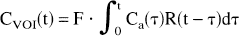
where C_a(t) is the arterial input, F is tissue blood flow, and R(t) is the vascular residue function (i.e., the fraction of tracer present in the vascular bed of the VOI at time t after injection of a unit impulse of tracer in its supply vessel). By treating the residue function as an unknown variable, this approach circumvents the problems of using intravascular tracers for CBF measurements pointed out by Lassen (1984) and Weisskoff et al. (1994).

Assuming that tissue and arterial concentrations are measured at equidistant time points t₁, t₂ = t₁ + Δt, …, t_N, this equation can be reformulated as a matrix equation

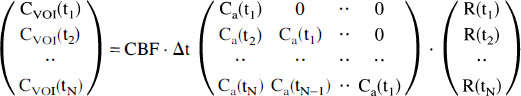
(\begin{matrix} C_{V O I} (t_{1}) \\ C_{V O I} (t_{2}) \\ \cdot \cdot \\ C_{V O I} (t_{N}) \end{matrix}) = C B F \cdot Δ t (\begin{matrix} C_{a} (t_{1}) & 0 & \cdot \cdot & 0 \\ C_{a} (t_{2}) & C_{a} (t_{1}) & \cdot \cdot & 0 \\ \cdot \cdot & \cdot \cdot & \cdot \cdot & \cdot \cdot \\ C_{a} (t_{N}) & C_{a} (t_{N - 1}) & \cdot \cdot & C_{a} (t_{1}) \end{matrix}) \cdot (\begin{matrix} R (t_{1}) \\ R (t_{2}) \\ \cdot \cdot \\ R (t_{N}) \end{matrix})

(2)

and solved for CBF · R(t) by algorithms from linear algebra. Østergaard et al. (1996a) demonstrated that by using singular value decomposition, R(t) and CBF can be determined with reasonable accuracy, independent of the underlying vascular structure and volume, and with raw image signal-to-noise ratios equivalent to those obtainable in current clinical MRI protocols.

Magnetic resonance imaging cerebral blood volume measurement

Vascular volume was determined by numerically integrating the area under the concentration time curve during the contrast bolus

{C B V}^{\propto} \int_{b o l u s} C_{V O I} (τ) d τ

(3)

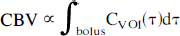
(Stewart, 1894). Absolute tracer concentrations are not readily available by means of the susceptibility contrast measurements used in this study (see Materials and Methods). However, because CBF and CBV are obtained from the same arbitrary concentration units, the empirical constant that yields true, absolute CBF found in the present study will also provide absolute CBV values.

Positron emission tomography cerebral blood flow measurement

The regional uptake of a diffusible tracer is described by the equation introduced by Ohta et al. (1996):

C_{V O I} (t) = (1 - V_{0}) \cdot K_{1} \cdot \int_{0}^{t} C_{a} (τ) e^{- k_{2} (t - τ)} d τ + V_{0} \cdot C_{a} (t)

(4)

where, by assumption, K₁ = CBF for freely diffusible tracers and k₂ = K₁/V_e, where V_e is the partition volume of the tracer. V₀ is the vascular distribution volume for the tracer in the tissue.

MATERIALS AND METHODS

Animal preparation and experimental protocol

Six female country-bred Yorkshire pigs weighing 38 to 45 kg were used in the experiments. Before the experiment, the pigs were housed singly in stalls in a thermostatically controlled (20°C) animal colony with natural lighting conditions. The pigs had free access to water but were deprived of food for 24 hours before the experiment. The project was approved by the Danish National Committee for Ethics in Animal Research. Pigs initially were sedated by intramuscular injection of 0.25 mL/kg of a mixture of midazolam (2.5 mg/mL) and ketamine hydrochloride (25 mg/mL). A catheter then was placed in an ear vein. After intravenous injection of additional midazolam/ketamine mixture (0.25 mL/kg), the pig was intubated and artificially ventilated (Engström Ventilator, Stockholm, Sweden) throughout the experiment, maintaining anesthesia by continuous infusion of 0.5 mL/kg per hour of the midazolam/ketamine mixture and 0.1 mg/kg per hour of pancuronium. Indwelling femoral arterial and venous catheters (Avanti size 4–7 French) were installed surgically. Infusions of isotonic saline (approximately 100 mL/hr) and 5% glucose (approximately 20 mL/hr) were administered intravenously throughout the experiments. Throughout the PET experiment, body temperature, blood pressure, heart rate, and expired-air carbon dioxide (CO₂) levels were monitored continuously (Kivex, Ballerup, Denmark), and arterial blood samples were withdrawn and analyzed (ABL 300, Radiometer, Copenhagen, Denmark) at regular intervals to monitor blood gases and whole blood acid—base parameters. In the magnetic resonance scanner, expired-air CO₂ levels were monitored continuously (Datex Normocap 200, Instrumentarium, Helsinki, Finland). Hypercapnia was induced by decreasing respiratory rate and tidal volume. The animal was allowed 1 hour to equilibrate to a steady arterial partial pressure CO₂ (P_aCO₂) level. At the end of experiment, the anesthetized pigs were killed in accordance with the regulations of the Danish National Ethics Committee for Animal Experiments.

Magnetic resonance imaging protocol

Imaging was performed using a GE Signa Horizon 1.0 Tesla Imager (GE Medical Systems, Milwaukee, WI, U.S.A.). After a sagittal scout, a T₁-weighted three-dimensional gradient echo sequence (time of repetition [TR] = 8 ms, time of echo [TE] = 1.5 ms, 20-degree flip angle) was acquired for later coregistration of MRI and PET data. For dynamic imaging of bolus passages, spin echo (TR = 1000 ms, TE = 75 ms) single-shot EPI was performed, starting 30 seconds before injection. A 64 × 64 acquisition matrix was used with a 14 × 14 cm coronal field of view, leading to an in-plane resolution of 2.2 × 2.2 mm². The slice thickness was 6 mm.

In all experiments, bolus injection of 0.2 mmol/kg gadodiamide (OMNISCAN, Nycomed Imaging, Oslo, Norway) was performed manually at a rate of 15 to 20 mL per second. Before the first dose, a predose of 0.05 mmol/kg was given to avoid systematic effects from changes in blood T₁.

Magnetic resonance imaging analysis

We used susceptibility contrast arising from compartmentalization of the paramagnetic contrast agent (Villringer et al., 1988) to determine tissue and arterial tracer levels. We assumed a linear relationship (Weisskoff et al., 1994) between paramagnetic contrast agent concentration and the change in transverse relaxation rate, Δ R₂, to determine tissue and arterial tracer time concentration curves C(t) according to the equation

C (t) \propto Δ R_{2} (t) = - \log (\frac{S (t)}{S (0)}) / T E

(5)

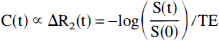
where S(0) and S(t) are the signal intensities at baseline and time t, respectively. We assumed T₁ to be unaltered during the bolus injection. This equation does not provide absolute concentrations. In our approach, we fixed the relation between susceptibility contrast and tracer concentration by requiring MRI flow rates in susceptibility contrast units to equal absolute flow rates measured by PET. The resulting constant of proportionality, Φ_Gd, is then used to calibrate MRI measurements of both CBF and CBV to absolute values.

The arterial concentration was determined in each animal from pixels containing large, feeding vessels (typically the middle cerebral artery) showing an early and large (3–10 times that of gray and white matter) ΔR₂ after contrast injection. This method has been demonstrated previously to closely reflect actual arterial levels for the susceptibility contrast agents used in this study when imaged using spin echo EPI techniques (Porkka et al., 1991). The integrated area of the arterial input curve was in each measurement normalized to the injected contrast dose (in mmol per kg body weight) to compare within and among animals.

To determine CBF from equation 2, the deconvolution was performed over the range of measurements, where the arterial input values exceeded the noise level (usually approximately 15 seconds). Deconvolution followed smoothing of raw image data by a 3 × 3 uniform smoothing kernel. The maximum of the deconvolved response curve was assumed to be proportional to CBF. Cerebral blood volume was determined by numerically integrating the concentration time curve from bolus arrival to tracer recirculation.

Positron emission tomography radiochemistry

¹⁵O₂ was produced by the ¹⁴N(d,n)¹⁵O nuclear reaction by the bombardment of nitrogen gas with 8.4 MeV deuterons using a GE PETtrace 200 cyclotron (Uppsala, Sweden). ¹⁵O₂ was mixed with hydrogen and passed in a stream of nitrogen gas over a palladium catalyst at 150°C to produce ¹⁵O-water vapor, which was trapped in 10 mL of sterile saline. ¹⁵O-CO was prepared by passing ¹⁵O₂ in a stream of nitrogen gas over activated carbon at 900°C. The ¹⁵O-CO was piped directly to a 500-mL vial in a dose calibrator situated close to the PET scanner. On decay to the required radioactivity, the ¹⁵0-CO was administered to the pig as described in the following section. ¹⁵O-Butanol was prepared by the reduction of ¹⁵O₂ with tri-n-butyl borane immobilized on an aluminum solid-phase matrix. The product was purified by transfer of the resulting radioactivity with 10 mL water onto a C18 solid phase extraction column. The ¹⁵O-butanol subsequently was eluted into a sterile vial with 10 mL of 20% ethanol.

Positron emission tomography imaging protocol

The pigs were studied lying supine in the scanner (Siemens/CTI ECAT EXACT HR) with the head in a custom-made head-holder. The position of the head was checked throughout the experiment with laser markers. To measure CBF, intravenous injection of 800 MBq H₂¹⁵O was performed, followed immediately by an intravenous injection of 3 to 4 mL of heparin solution (20 international units/L isotonic saline) to flush the catheter. We acquired a sequence of 21 (one sample every 5th second for 1 minute, one sample every 10th second for 1 minute, and one sample every 20th second for 1 minute) arterial blood samples (1–2 mL) and 12 PET brain images (one image every 10th second for 1 minute, one image every 15th second for 1 minute, and one image every 30th second for the remaining minute). To measure CBV, we administered 800 MBq ¹⁵O-labeled CO mixed with oxygen to a 1-L volume by syringe. After 10 seconds breath-hold, normal ventilation resumed. To assess the variability of repeated CBF results, an additional injection of ¹⁵O-butanol was performed in one pig, using the aforementioned imaging and blood sampling scheme. For all experiments, total radioactivity in blood samples was measured, and image as well as arterial data were corrected for the half-life of ¹⁵O (123 seconds). Positron emission tomography image data were reconstructed using a Hanning filter with a cutoff frequency of 0.5 pixel⁻¹, resulting in a spatial resolution full width at half maximum (FWHM) of 4.6 mm. Correction for attenuation was made on the basis of the transmission scan.

Positron emission tomography image analysis

High signal-to-noise ratio PET data were used to coregister PET and MRI data using REGISTER (courtesy David McDonald and Peter Neelin, Montreal Neurological Institute, McGill University, Montreal, Canada). Raw PET image data then were transformed and resampled to the same spatial location and resolution as the MRI data to allow direct comparison of the two techniques. After the application of the 3 × 3 uniform smoothing kernel to the raw PET images, the ¹⁵O water data were fitted to equation 4 using nonlinear, least-squared regression analysis of each image voxel. Cerebral blood volume was determined by the ratio of cerebral and arterial whole blood ¹⁵O CO levels after initial distribution (30 seconds) of the tracer. We assumed that the mean brain-to-systemic hematocrit ratio is 0.69 (Lammertsma et al., 1984). To correct for slightly different Paco₂ levels in the MRI and PET normo- and hypercapnic conditions, respectively, the PET CBF and CBV maps were corrected to the Paco₂ of the MRI measurements. We assumed a linear relationship between Paco₂, and CBV and CBF, respectively (Grubb et al., 1974), that is

C B F = a \cdot {P a c o}_{2} + b

The two constants a and b were determined for each pixel, and CBV and CBF were corrected.

Comparison of positron emission tomography and magnetic resonance imaging parameter images

Magnetic resonance imaging CBF maps were filtered using a 4.5-mm FWHM Gaussian filter to make the spatial resolution of PET and MRI maps as similar as possible. Pixel maps of CBF (at similar anatomic locations and pixel size) generated with PET and MRI then were compared on a regional basis for the normo- and hypercapnic condition. In each image, 10 to 12 regions of interest of similar size were chosen. Average regional CBF values and their standard deviations (SDs) (derived from the pixels within the region of interest) for the normo- and hypercapnic conditions then were plotted versus the corresponding PET CBF values to examine the appropriateness of a linear relationship between the two estimates. Linear least-squared regression analysis was performed to determine the slope and y intercept of the linear fit. Finally, to test whether a common conversion factor yields absolute CBF by MRI, Student's t-tests were performed, comparing the slope and its SD for each pig with those of the remaining pigs.

RESULTS

By averaging regional MRI CBF values (as determined by equations 2 and 5) and ¹⁵O water PET CBF values (in mL/100 mL/min) for all pigs (for both normo- and hypercapnic conditions), a conversion factor of Φ_Gd = 1.09 was found. In the remaining analysis, all MRI flow rates were multiplied by this factor.

Figure 1 shows parametric maps of CBF for pig 3. The pixel size is the same in the two images. Notice the good overall agreement between the regional values and responses to arterial CO₂ levels using the two methods, although the MRI CBF map appears to distinguish better between gray and white matter structures than the PET CBF maps. Also, the PET CBF map appears to be somewhat noisier than the MRI CBF map. We investigated possible regional differences in CBF maps obtained by the two methods. These appeared to be mainly associated with either noise artifacts or the presence of veins in the PET image slice. Noise in PET images appears as “streaky artifacts” that sometimes propagate into the CBF maps. Conversely, veins often are interpreted by the kinetic model in equation 4 as a high flow region, whereas they rarely are detected by the MRI sequence.

FIG. 1.

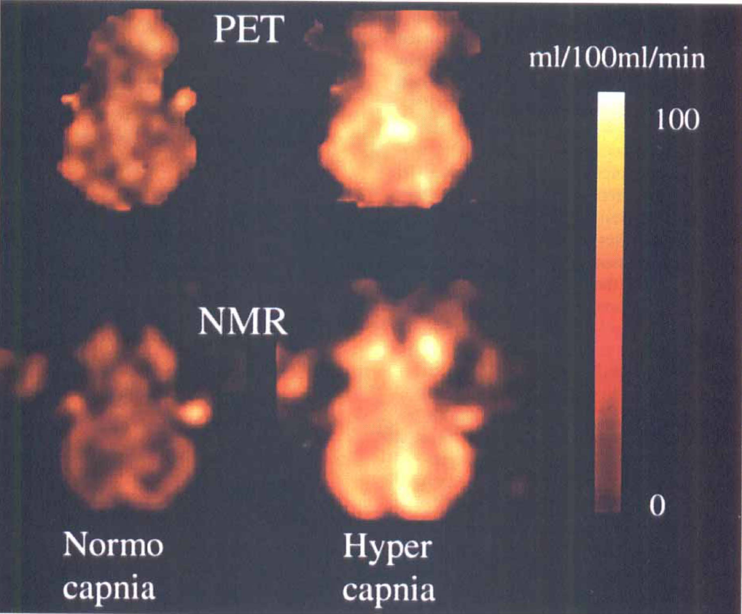
Parametric cerebral blood flow maps using positron emission tomography (top row) and magnetic resonance imaging (bottom) for normocapnia (left) and hypercapnia (right), respectively, in pig 3.

Figure 2 shows plots of regional CBF values with their SDs for individual pigs. Notice that normo- and hypercapnic data points are plotted in the same diagram to visualize overall agreement of absolute values, as well as responses to CO₂ among PET and MRI. There was a tendency for normocapnic data points to be grouped in the lower left and hypercapnic data points in the upper right quadrant of the plots. The error bars associated with the MRI measurements appear smaller than the corresponding PET values for the same region. The average SD on regional flow estimates was approximately 30% smaller than the corresponding SD for the same PET region of interest. Figure 3 shows the corresponding plot for repeated PET measurement of CBF with ¹⁵O butanol. The results of the linear regression analysis are shown in Table 1. The slopes of the linear regression lines did not significantly differ among the pigs (by multiple pairwise Student's t tests). For most animals, the regression coefficient r² (the proportion of the variance accounted for by the regression) ranged between 0.7 and 0.8. This was slightly lower than the value (i.e., 0.86) obtained by comparing CBF maps obtained in identical brain slices with PET. Hence, the additional inaccuracies introduced by comparing CBF determined by two different methods therefore are small compared with the variance associated with comparisons made within the same method.

TABLE 1.

Linear regression results for six pigs

Pig	a	b	r²
1	0.88 ± 0.11	8 ± 5	0.80
2	1.00 ± 0.11	−2 ± 6	0.81
3	0.99 ± 0.15	0 ± 10	0.70
4	0.97 ± 0.11	−4 ± 6	0.79
5	0.98 ± 0.11	2 ± 7	0.81
6	0.90 ± 0.12	6 ± 5	0.75
6*	0.77 ± 0.07	10 ± 3	0.86

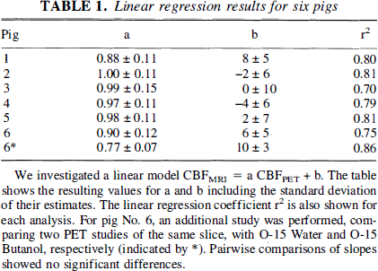
We investigated a linear model CBF_MRI = a CBF_PET + b. The table shows the resulting values for a and b including the standard deviation of their estimates. The linear regression coefficient r² is also shown for each analysis. For pig No. 6, an additional study was performed, comparing two PET studies of the same slice, with O-15 Water and O-15 Butanol, respectively (indicated by *). Pairwise comparisons of slopes showed no significant differences.

FIG. 2.

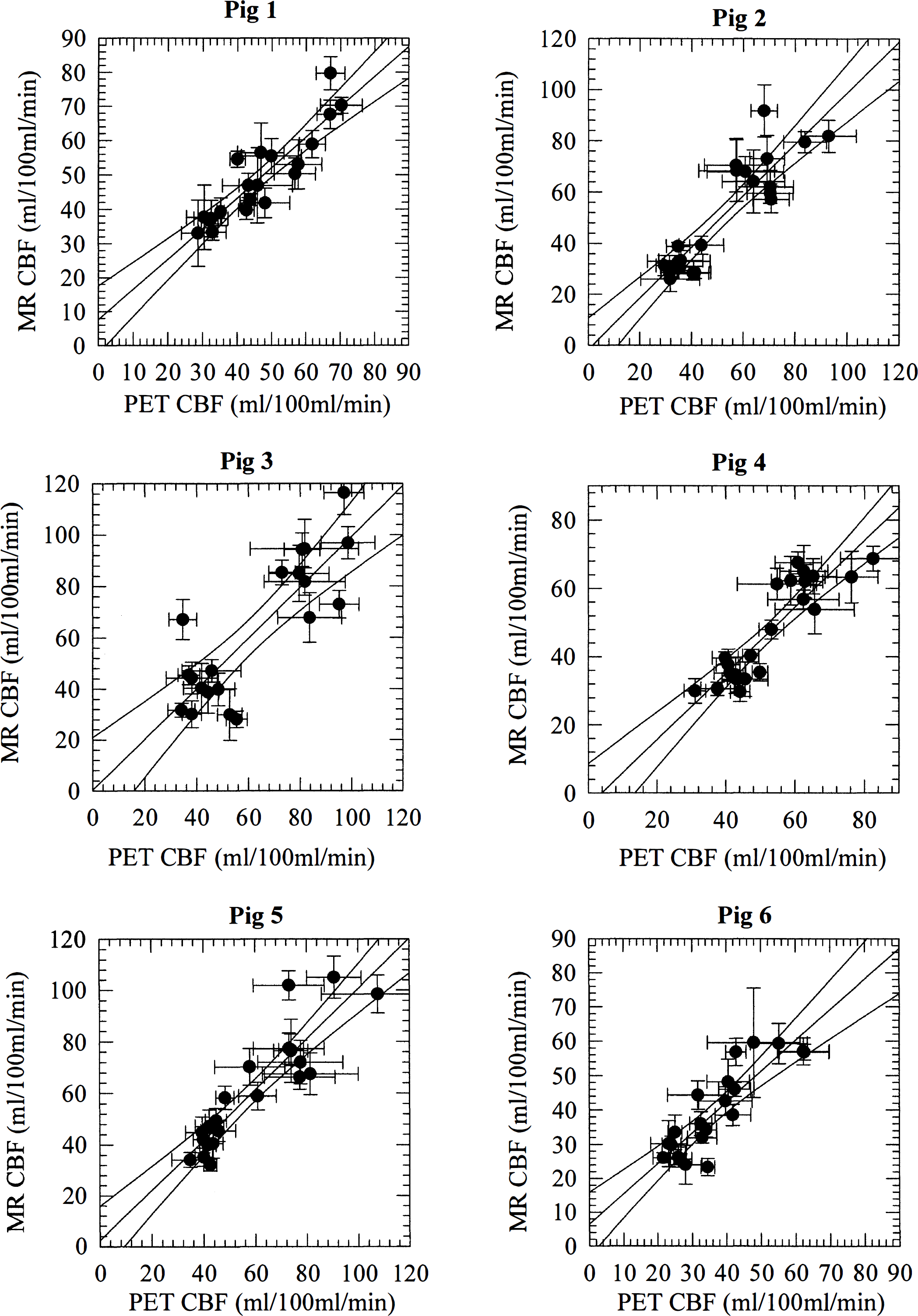
Correlation between regional positron emission tomography and magnetic resonance imaging cerebral blood flow values. The linear regression lines and their 95% confidence intervals also are shown.

FIG. 3.

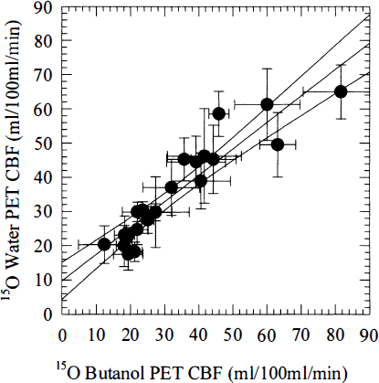
Correlation between regional positron emission tomography (PET) cerebral blood flow values determined by ¹⁵CD-labeled water and butanol, respectively, in pig 6. The arterial partial pressure of carbon dioxide (Paco₂) levels were identical during the respective measurements. The linear regression line and its 95% confidence interval are shown. Notice the slope is somewhat lower than 1.0 because of the poorer reproduction of high flow rates with H₂¹⁵O PET.

Figure 4 shows CBV maps obtained with MRI and PET, respectively. Because CBV and CBF are obtained in the same units, absolute CBV values were obtained by multiplying the integrated value by the normalization factor Φ_Gd = 1.09, determined above. Figure 5 plots average absolute MRI versus PET values of CBV for corresponding slices under normo- and hypercapnia in six pigs. Care was taken to include brain parenchyma rather than large vessels in the image. Also shown is the linear regression line with slope 0.45 ± 0.11 (SD) and y intercept −0.56 ± 0.61 (SD). Notice the apparent linearity between vascular volume measurements with PET and MRI. Because both MRI and PET CBV values are in absolute values, the plot shows that only 40% of the total vascular volume is detected by the spin echo EPI MRI technique.

FIG. 4.

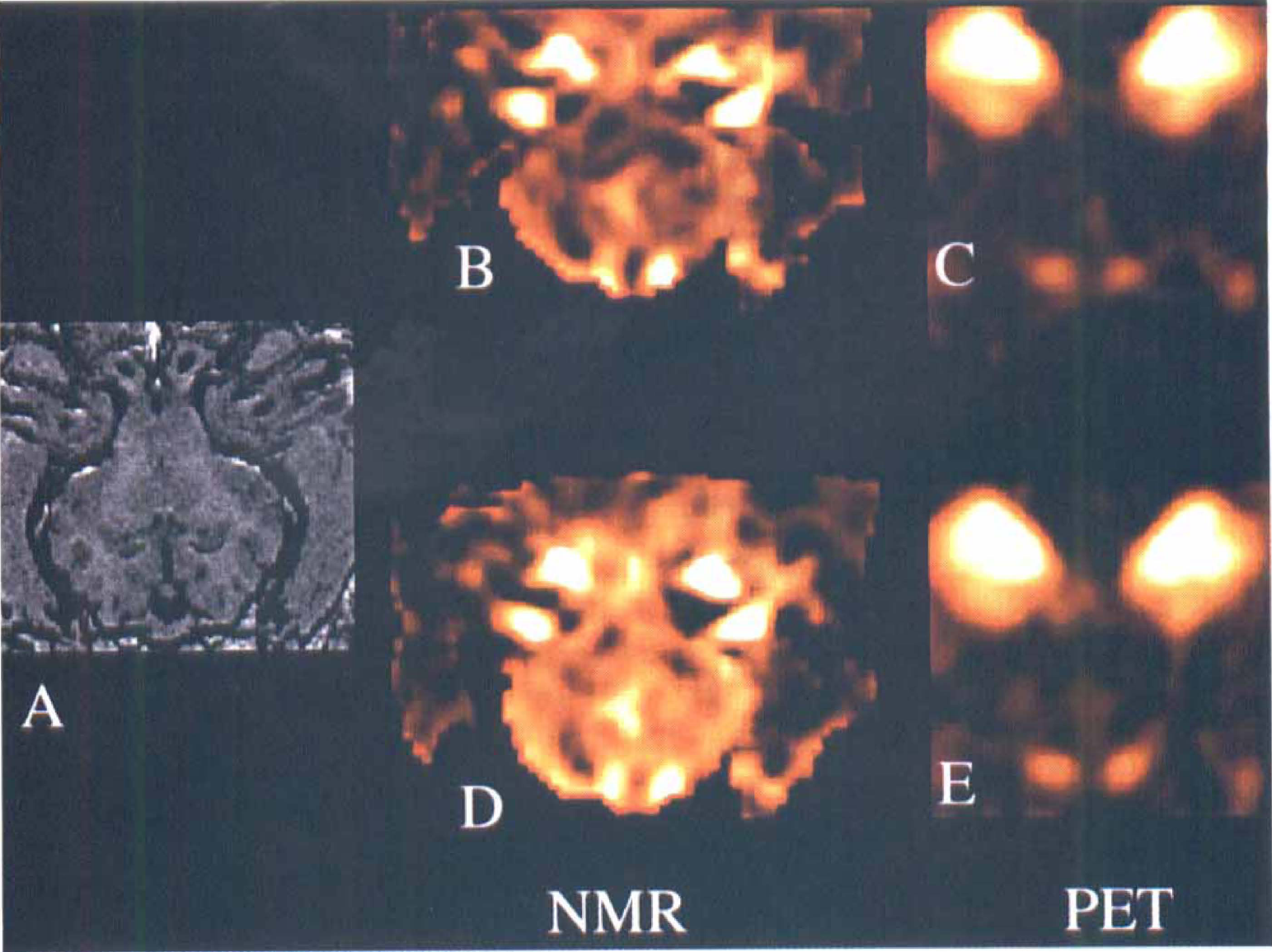
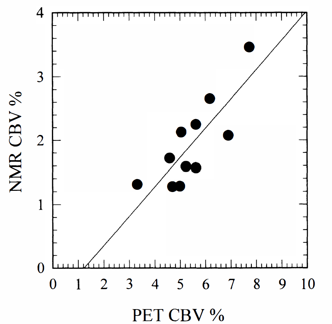
Parametric cerebral blood volume maps using positron emission tomography (PET) and magnetic resonance imaging (MRI) for the same brain slice (A) in normocapnia (B and C) and hypercapnia (D and E). The color scales are different to visualize the images. The large blood volumes in the veins behind the eye in the PET images are not visible by MRI. The transverse venous sinus is visualized by both PET and MRI.

FIG. 5.

Correlation between regional positron emission tomography and magnetic resonance imaging cerebral blood volume values. The regression line y = 0.46 × −0.56 (r² = 0.67) is shown.

DISCUSSION

Despite the inherent complexity of susceptibility contrast mechanisms and their use for measurements of CBF, our rather simple approach to quantify CBF from MRI seems promising as a first approach toward measurement of absolute CBF. In all six animals, the common conversion factor yielded absolute CBF values in surprisingly good agreement with those obtained by PET. Furthermore, the MRI technique yielded CBF maps with good contrast between gray and white matter structures, just as by regional comparison, MRI CBF maps had less noise than the corresponding PET CBF maps, using similar spatial resolution. Our assumptions and experimental approach may explain the poorer correlation between MRI and PET CBF results than among repeated PET CBF measurements.

First, assuming a common constant that relates injected MRI contrast dose to the area under the image-based arterial input concentration time curve may not always hold true. The validity of this assumption is sensitive to the fraction of the injected contrast dose delivered to the brain circulation in the two experimental conditions, and more importantly, the linearity between contrast concentration and change in transverse relaxation rate assumed in equation 5. Second, we assumed a linear relationship between CBF and arterial CO₂ levels when correcting for different degrees of hypercapnia in PET and MRI experiments. However, deviations from linearity may cause systematic changes in the slope and intercept of the regression line, just as the CO₂ response of the animal may change after long-term anesthesia (MRI measurements were performed approximately 4 hours after the PET measurements).

As for more methodologic problems, comparing MRI with PET may have affected our regression results in several ways. Coregistration of MRI and PET data may not be completely accurate, just as magnetic resonance images obtained with EPI can be somewhat distorted because of magnetic field inhomogeneities and susceptibility artifacts. The latter cause anatomic structures imaged by the EPI sequence not to be imaged in the exact location as in the three-dimensional image sequence used for coregistration. In cases in which we noticed slight in-plane differences in locations, we adjusted the location of the region of interest in the MRI images to account for this.

A more complex problem was caused by the differences in inherent resolutions of PET and MRI. For our PET system, the effective resolution with the parameters used is approximately 4.5 mm in the center of the investigated volume. By using a Gaussian filter, we sought to blur the MRI measurements to yield the same resolution as the PET CBF measurements. However, the CBF images in Figure 1 still indicate that there may be differences in resolution that are not accounted for, causing influence from neighboring regions to be different in the two imaging modalities, thereby causing a nonlinear relationship between regional CBF values simply because of differences in resolution. We believe that these factors explain the slightly better regression statistics obtained when comparing two PET CBF measurements rather than comparing MRI measurements. Some data sets (pigs 1 and 6) yielded regression lines with slopes somewhat below unity and a positive y-axis intercept, as also found when comparing ¹⁵O water and ¹⁵O butanol CBF measurements. With the latter tracer, the discrepancy is due to limited diffusibility of water across the blood—brain barrier, causing higher flows to be underestimated (Ohta et al., 1996). For MRI measurements, the earlier simulation studies also predicted that high flow rates would be underestimated, when the microvascular mean transit time is short relative to the characteristic time scales of the bolus input and the imaging rate (Østergaard et al., 1996). By very rapid bolus administration and imaging once per second, we hoped to minimize this effect. The results indicate that the MRI technique may perform slightly worse than the PET method with ¹⁵O water in terms of measuring very high flow rates.

The measurements provide insight into the selectivity for the effect of small vessels of the T₂-weighted spin echo EPI sequence used in our experiment. By a Monte Carlo simulation approach, Weisskoff et al. (1994) previously demonstrated that the susceptibility contrast in this imaging sequence arises mainly in small, capillary-sized vessels. Because the distribution of fractional vascular volume as a function of vascular diameter is not fully known, it is difficult to predict absolute volume values based on these simulations. Therefore, our 40% to 50% estimate of the vascular fraction detected by MRI is difficult to compare with theoretical predictions. However, studies of peripheral tissue indicate that vessels smaller than 30 to 40 μm in diameter (small arteries, arterioles, capillaries, venules, and small veins) represent approximately 50% of the total vascular volume (Johnson, 1973). Assuming that the MRI measurements are predominantly sensitive to the smallest vessels, our value of 40% to 50% therefore points toward a sensitivity of the MRI technique to vessels smaller than 30 to 40 μm. This in turn makes the CBF and CBV techniques sensitive to microvascular phenomena, for example, neovascularization in neoplasia (Aronen et al., 1994) and flow-volume mismatches in stroke due to delayed passage through oxygen-exchanging vessels (Heiss et al., 1994).

Footnotes

Abbreviations used

Acknowledgment

The authors thank Nycomed Imaging (Oslo, Norway) for providing the contrast agent for this study.

References

Aronen

Gazit

Louis

(1994) Cerebral blood volume maps of gliomas: comparison with tumor grade and histological findings. Radiology 191:41–51

Grubb

Raichle

Eichling

Ter-Pogossian

(1974) The effects of changes in P_aCO₂ on cerebral blood volume, blood flow, and vascular mean transit time. Stroke 5:630–639

Heiss

Graf

Wienhard

(1994) Dynamic penumbra demonstrated by sequential multitracer PET after middle cerebral artery occlusion in cats. J Cereb Blood Flow Metab 14:892–902

Johnson

(1973) Peripheral Circulation, New York: Wiley, p 3

Lammertsma

Brooks

Beaney

(1984) In vivo measurement of regional cerebral haematocrit using positron emission tomography. J Cereb Blood Flow Metab 4:317–322

Lassen

(1984) Cerebral transit of an intravascular tracer may allow measurement of regional blood volume but not regional flow. J Cereb Blood Flow Metab 4:633–634

Ohta

Meyer

Fujita

Reutens

Evans

Gjedde

(1996) Cerebral [¹⁵O] water clearance in humans determined by PET: I. Theory and normal values. J Cereb Blood Flow Metab 16:765–780

Porkka

Neuder

Hunter

Weisskoff

Belliveau

Rosen

(1991) Arterial input function measurement with MRI. In: Proc Soc Magn Reson Med, 10th Annual Meeting, San Francisco, p 120

Rosen

Belliveau

Vevea

Brady

(1990) Perfusion imaging with NMR contrast agents. Magn Reson Med 14:249–265

10.

Rosen

Belliveau

Buchbinder

(1991) Contrast agent and cerebral hemodynamics. Magn Reson Med 19:285–292

11.

Sorensen

Buonanno

Gonzalez

(1996) Hyperacute stroke: evaluation with combined multisection diffusion weighted and hemodynamically weighted echo-planar MR imaging. Radiology 199:391–401

12.

Stewart

(1894) Researches on the circulation time in organs and on the influences which affect it. Parts I—III. J Physiol (Lond) 15:1

13.

Villringer

Rosen

Belliveau

(1988) Dynamic imaging with lanthanide chelates in normal brain: contrast due to magnetic susceptibility effects. MRM 6:164–174

14.

Weisskoff

Chesler

Boxerman

Rosen

(1993) Pitfalls in MR measurements of tissue blood flow with intravascular tracers: which mean transit time? MRM 29:553–559

15.

Weisskoff

Zuo

Boxerman

Rosen

(1994) Microscopic susceptibility variation and transverse relaxation: theory and experiment. MRM 31:601–610

16.

Østergaard

Weisskoff

Chesler

Gyldensted

Rosen

(1996a) High resolution measurement of cerebral blood flow using intravascular tracer bolus passages: part I, mathematical approach and statistical analysis. MRM 36:715–715

17.

Østergaard

Sorensen

Kwong

Weisskoff

Gyldensted

Rosen

(1996b) High resolution measurement of cerebral blood flow using intravascular tracer bolus passages: part II, experimental comparison and preliminary results. MRM 36:726–736

Absolute Cerebral Blood Flow and Blood Volume Measured by Magnetic Resonance Imaging Bolus Tracking: Comparison with Positron Emission Tomography Values

Abstract

Keywords

THEORY

Magnetic resonance imaging cerebral blood flow measurements

Magnetic resonance imaging cerebral blood volume measurement

Positron emission tomography cerebral blood flow measurement

MATERIALS AND METHODS

Animal preparation and experimental protocol

Magnetic resonance imaging protocol

Magnetic resonance imaging analysis

Positron emission tomography radiochemistry

Positron emission tomography imaging protocol

Positron emission tomography image analysis

Comparison of positron emission tomography and magnetic resonance imaging parameter images

RESULTS

DISCUSSION

Footnotes

Abbreviations used

Acknowledgment

References