Performance of a Randomization Test for Single-Subject 15 O-Water PET Activation Studies

Abstract

We adapted and implemented a permutation test (Holmes 1994) to single-subject positron emission tomography (PET) activation studies with multiple replications of conditions. That test determines the experimentwise α error as well as location and extent of focal activations in each individual. Its performance was assessed in five normal volunteers, using ¹⁵O-H2O-PET data acquired on a high-resolution scanner, with septa retracted (3D mode), during functional activation by repeating words versus resting (four replications each). Calculated α errors decreased and the size of activated tissue volumes (voxels with P ≤ 0.05) increased with increasing filter kernel size applied to the difference images. At a filter kernel of 12 mm Gaussian full width at half maximum, significant focal activations were seen bilaterally in superior temporal cortex, including Brodmann's areas 41 and 42, in all five subjects. Additional foci were detected in the precentral gyrus, left inferior frontal gyrus, supplementary motor area, and cerebellum of several subjects. The average CBF increase in activated voxels ranged from 17.6% to 28.7%. Activated volumes were smaller than those detected with a standard parametric test procedure. We conclude that the permutation test is a less sensitive procedure, having the advantage of not depending on unproven distributional assumptions, that detects strong activation foci in individual subjects with high reproducibility.

Positron emission tomography (PET) studies on brain function are often evaluated by parametric methods involving PET images modeled as continuous random fields (Friston et al. 1991, Worsley et al. 1992). This implies numerous assumptions that are difficult to prove because of the noise in the data and the small number of scans. Additional pitfalls are the statistical dependence of adjacent voxels, long-range correlations between functionally connected brain areas, and noisy variance estimates with unknown properties, on which Ford (1995) commented that the common assumption of voxel-level variance homogeneity is untenable. Therefore, Holmes (1994) and Holmes et al. (1996) developed a nonparametric method for the significance testing of functional PET images, replacing the formal assumptions mentioned above by great computational effort that became manageable with modern processor technology. The main idea is to change labeling of the images as “rest” or “activation” and test whether the statistic describing the activation changes in comparison with other labeling permutations. Thus, a nonparametric threshold test can be applied to the calculated rank value. Holmes (1994) claimed that only minimal assumptions are involved and that the type I error is exactly that specified (except for rounding errors), leading to a test that is always valid. Whereas Holmes used t-statistic images formed with smoothed variance images, he stated that the absence of distributional assumptions permits the consideration of a wide range of test statistics. In addition, the permutation applied to scans from different subjects can as well be applied to a single-subject activation experiment. In order to test this, we evaluated permuted normalized difference images for significance detection in single-subject ¹⁵O-H₂O-PET activation studies.

MATERIALS AND METHODS

Basics of permutation testing

We used the principles of the permutation test as described by Holmes (1994). It can be summarized as follows: Let Ω be the set of intracerebral voxels measured in a functional brain activation experiment in which half of the scans have been acquired under condition A and the other half under condition B. In our application, as the simplest measure of activation, we used a statistic image T formed by subtracting the mean voxel values for condition A (rest) from the mean of those for condition B (activation). The null hypothesis H₀ states that for each voxel k∈Ω, each condition would have produced the same mean value were the conditions of this scan reversed, implying that voxel k shows no activation at all. Consequently, if the labeling of the scans does not matter, each statistic image T (see implementation below) formed by randomizing the labels between scans is as likely as the observed one. For n scans, there are N = n!/(n/2)!² possible relabelings, holding the proposition that half of the scans were taken under each condition, thus providing a counterbalanced sequence. To reject H₀, it is sufficient to consider the maximum observed statistic derived from the statistic image T, because if the maximum fails to reject H₀, no other voxel will:

$$T_{max}=max\{T(k):k\in \Omega \}$$

Because under H₀ the probability that T_max is any one of the maxima t_maxi derived from each possible labeling i(i = 1, …, N) is equally likely, the probability of observing a statistic image with a maximum value equal to or greater than T_max is the proportion of t_maxi equal to or greater than T_max. In the general case of a level a test, the critical value should be chosen as the 100(1 – α)th percentile of t_maxi, tc, by choosing the rank threshold c as (αN) rounded down: c = ⌊αN⌋. The observed statistic image T can thus be set at a threshold that declares all voxels with values greater than the critical value as activated. The probability of type I error therefore is simply calculated as:

$$Pr(T_{max}>t_c|H_0)⩽c/N=\lfloor \alpha N\rfloor /N⩽\alpha$$

To prevent a major activation focus from considerably raising the maximal statistic and hence increasing the critical value of the test, the test is extended to a sequentially rejective version as described by Holm (1979), resulting in the following step-down approach: activated voxels are identified as described above and are cut out, and the remainder of the volume of interest is analyzed. The process iterates until no more activated voxels are found. Each test “protects” those following it, as each test must reject the omnibus null hypothesis for the remaining region in order to proceed to subsequent tests. Finally, a probablilty value adjustment is made for each voxel by enforcing monotonicity of the probability values computed after each step. The adjustment is necessary to ensure that no voxel can be assigned a lower a probability than another voxel already cut out in the iteration process. By accumulating the proportions for the adjusted probability values as suggested by Westfall and Young (1993), as each randomized statistic image is computed the calculation can be done more efficiently. The resulting algorithm is:

• 1)

  Let w be the number of intracerebral voxels. Let k₁, …, k_w be the intracerebral voxels ordered such that their values in the observed (nonpermuted) statistic image T go from smallest, T(k₁), to largest, T(k_w).

• 2)

  For j = 1, …, w: Let counting variable C_j = 0. It represents the number of combinations resulting in larger statistic values than the observed one. Let combination counting variable i = l.

• 3)

  Generate the statistic image ti corresponding to rerandomization i of the labels, not including the observed image.

• 4)

  Form the successive maxima: v_I = ti(k1); for j = 2, …, w: v_j = max[v_{j − 1}, ti(kj)]

• 5)

  For j = 1, …, w: If v _j ≥ T(k_j) then increment C_j by one. This comparison together with the previous monotonicity enforcing step implements the cutting out feature of the step-down algorithm.

• 6)

  Repeat steps 3 through 5 for each remaining possible relabeling i = 2, …, N.

• 7)

  Compute preliminary P values: For j = 1, …, w: P′(k_j) = (C_j + 1)/N.

• 8)

  Enforce monotonicity of P values: P = P′; for j = w − 1, …, 1: P(kj) = max[P(kj + 1), P(kj)]

Implementation of randomization test

The program we wrote to implement the randomization test for single-case multiscan PET studies, nicknamed Sherlock, was written in ANSI C and implemented on the Solaris 2.4 platform (Sun Microsystems Inc, Palo Alto, CA, U.S.A.) on a SparcStation 10. The program's input consists of a multiframe MATRIX file containing the subject's scans, the description of the rest/activation/ignore property of each scan, the mask file defining the intracerebral voxels together with a threshold for this purpose, and finally a filter kernel size. The program delivers two images, stored in the original MATRIX file format for further processing and display: one (*d) for the filtered difference image, and the other (*p) for the step-down adjusted type I error probability as detailed above. The latter image, called probability image, is the basis for subsequent analysis.

PET procedure

We studied five healthy normal subjects, three men and two women (27, 65, 69, 68, and 52 years old), to whom the study purpose and procedure, including the radiation dose, was explained in detail. All gave their written informed consent. Every subject was clearly right-handed as determined by the Edinburgh inventory, with the exception of one women (P3) born left-handed, whose right-handedness was enforced during education. The study was part of an investigation that was approved by the ethics committee of the medical faculty of the University of Cologne. From each subject, eight sets of PET images were acquired: four in a standard resting condition (A), and four while repeating common German nouns at a self-paced rate (B), resulting in an average of 51 (range, 43 to 60) words in 90 seconds. Data acquisition time was 90 seconds after injection of 370 MBq ¹⁵O-H₂O. The paradigm was administered with the subjects' eyes closed and ears unplugged, and with a low background noise in a dimly lit room. We used the mixed sequence ABBABAAB to protect the experimental design against confounding time effects. The subjects were instructed to relax as much as possible for resting, and to repeat the words clearly, audibly, and as fast as possible for the activation runs. Positron emission data acquisition was performed on a high-resolution scanner (ECAT EXACT HR 961, Siemens/CTI, Knoxville, TN, U.S.A.) in 3D mode, as described in detail by Wienhard et al. (1994).

Image processing

All intra-subject scans were aligned to the first scan using the fully automated procedure of Woods et al. (1992). The mean image of those aligned scans was rotated into a standard position defined by an average 2-(¹⁸F)fluoro-2-deoxy-d-glucose scan in anterior commissure-posterior commissure orientation, using the visually controlled procedure described by Pietrzyk et al. (1990). All intra-subject scans were then aligned again to the AC-PC-oriented mean image of the first alignment. As a last manually performed step, a mask defining all cerebral voxels was created by choosing a threshold right above the scalp activity and manually cutting out extracerebral (i.e., vascular) voxels with our standard software, especially at the base of the brain. After spatial filtering with a Gaussian filter kernel to increase the signal-to-noise ratio, as described in the results below, the randomization test was performed as described above, including linear scaling of the voxel values of each scan to the global average. Additionally, the probability image resulting from the permutation test was transformed into stereotactic space, facilitating comparison with other studies.

Finally, the aligned scans were also evaluated using the Standard Parametric Mapping version 95 package by Friston et al. (1991). For this procedure, standard options were used, namely a gray matter threshold of 0.8, linear scaling of voxels to a global average of 50, and a contrast vector of [–1, 1] for rest and activation scans, respectively. The SPM Z-statistic image was set at a threshold of Z = 1.64, corresponding to P = 0.05 as in the randomization test. A recently introduced additional correction for spatial extent (Friston et al. 1994) was not used, because the validation of this approach is the subject of current work (Friston, 1995) and would spoil the comparability of our results. Thus, the multiple comparison correction inherent in the step-down approach of the permutation test was paralleled by the SPM smoothness correction performed by estimating the number of resolution elements comprising the intracerebral space.

RESULTS

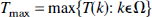
The number of voxels found to be significantly activated depends on the chosen filter kernel size, as demonstrated in Fig. 1. Only very little activation was seen in three subjects at filter sizes of 10-mm FWHM or less. The increase in the number of activated voxels was mainly caused by enlargement of contiguous activated volumes. Therefore it is clear that localization is blurred to such a degree as to render the finding practically useless when the filter kernel is in the order of magnitude of major cortical structures. A filter size of 12-mm FWHM produced the most reasonable results with regard to the extent of the main activation focus along the superior temporal gyrus, whereas larger filter sizes caused blurring of this region across the Sylvian fissure. Thus, the latter filter size was used for subsequent analysis.

Fig. 1.

Each curve represents the number of significant voxels plotted against the filter kernel size represented as Gaussian full width at half maximum in mm of the Gaussian filter kernel used for each subject. The strong dependence of the activated area on the filter kernel size is obvious.

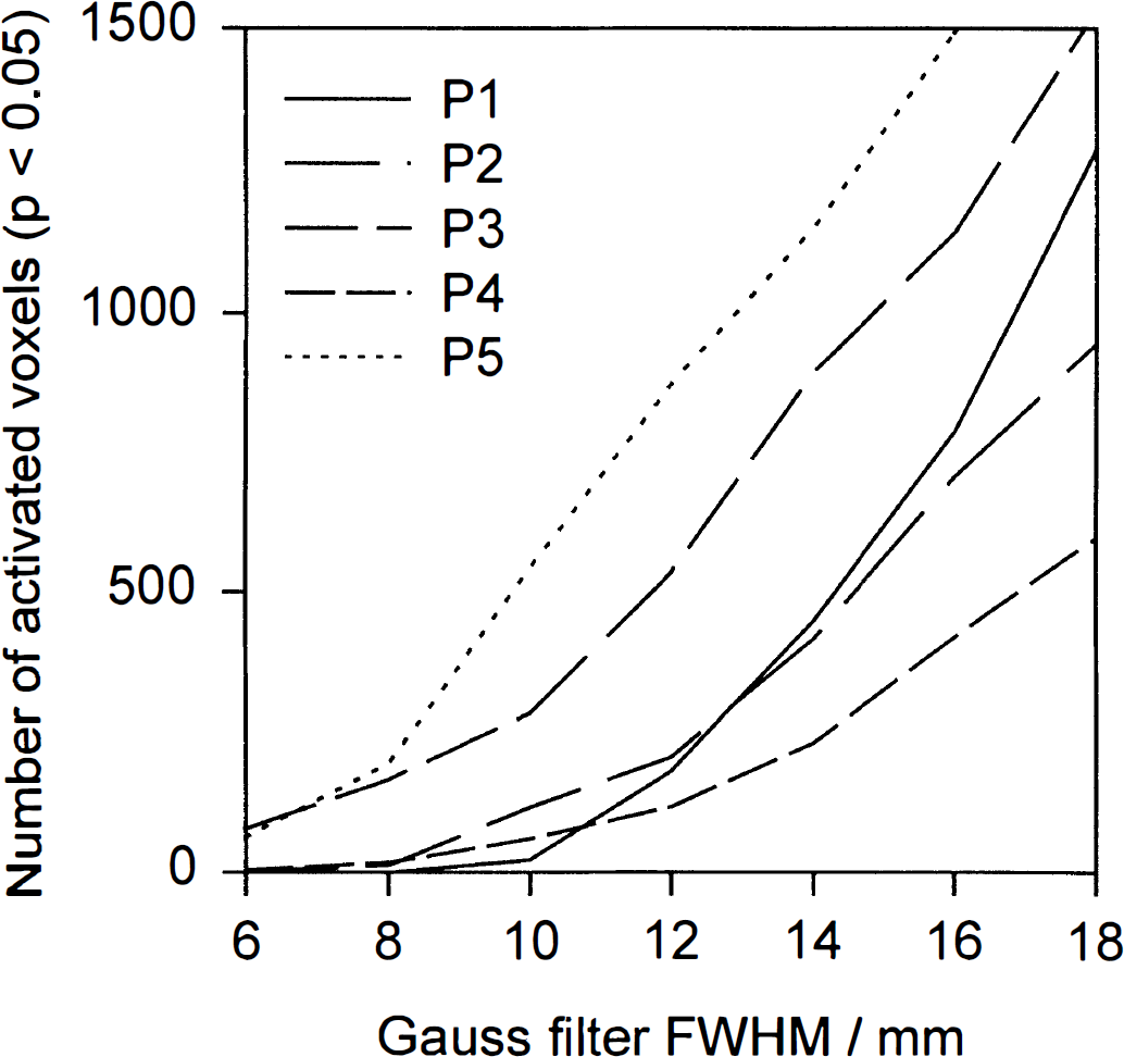
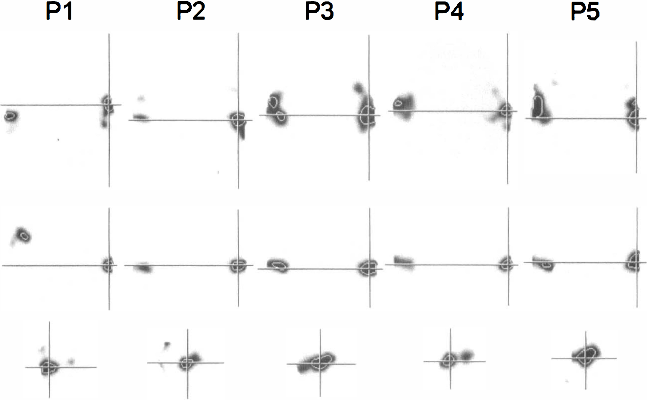
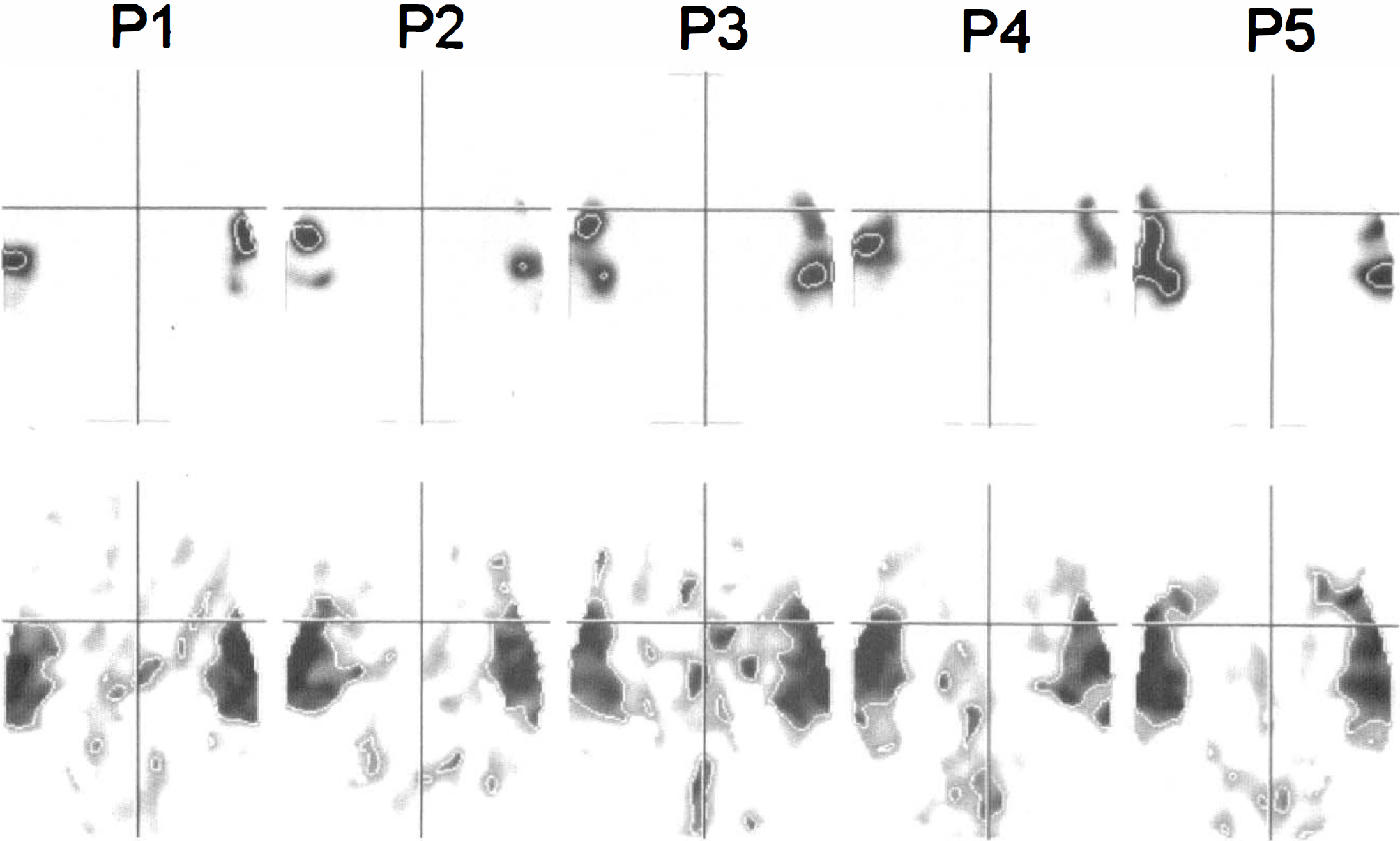
Cortical areas of activation comprised the posterior part of the superior temporal gyrus, including parts of Brodmann's areas 41, 42, and 22 bilaterally in all subjects. Vocalization areas (lower part of the precentral gyrus), inferior frontal gyrus (Brodmann's areas 44 and 45), supplementary motor area, and cerebellar activations were seen with varying probability and extent (Table 1). The sections across the posterior part of the left superior temporal gyrus on the a probability images resulting from the randomization test are shown in Figure 2. The maximum intensity projection maps based on the SPM Z-statistic at a threshold of 0.05 (Z > 1.64, df = 6) for each of the five subjects are shown in Figure 3. For direct comparison, a sample slice taken from the resampled and stereotactically transformed randomization test result at 8 mm above the AC-PC line, together with the corresponding SPM{Z}, had a thresholded at 0.05, as shown in Figure 4. The activated areas detected by SPM95 were much larger than those detected by the randomization test. In the latter, the activated volumes were relatively compact, whereas with SPM95 borders were more irregular and comprised association cortex and subcortical structures, too.

Fig. 2.

Permutation test results, represented in three orthogonal sections: darker shading means lower α probability; areas reaching 0.05 or less are delineated by a thin white line, thus representing the voxels considered to be significantly activated by the paradigm used. The cut shown here was made through the region of the lowest α probability in the posterior part of the left superior temporal gyrus.

Fig. 3.

Maximum intensity projection maps produced by Standard Parametric Mapping version 95 with a threshold of 0.05 (Z > 1.64, df = 6), as used most frequently in the literature, resulting in a quite liberal significance threshold.

Fig. 4.

A sample slice taken at 8 mm above the anterior commissure-posterior commissure line together with the corresponding SPM {2} thresholded at P = 0.05, facilitating comparison of the two approaches.

Table 1.

Lowest alpha probability found in each activation region as defined anatomically on coregistered MR image

		P1	P2	P3	P4	P5
Superior temporal gyrus	L	0.01	0.01	0.01	0.01	0.01
(Brodmann's area 42 + 42)	R	0.01	0.01	0.01	0.01	0.01
Precentral gyrus	L	0.36	0.01	0.01	0.31	0.22
(Brodmann's area 4)	R	0.01	0.19	—	0.16	0.83
Inferior frontal gyrus	L	—	—	0.24	—	0.04
(Brodmann's area 44)	R	—	—	—	—	—
Superior frontal gyrus
(supplementary motor area)	0.31	0.01	0.79	*	0.28
Cerebellum		0.71	0.10	0.01	0.17	0.09

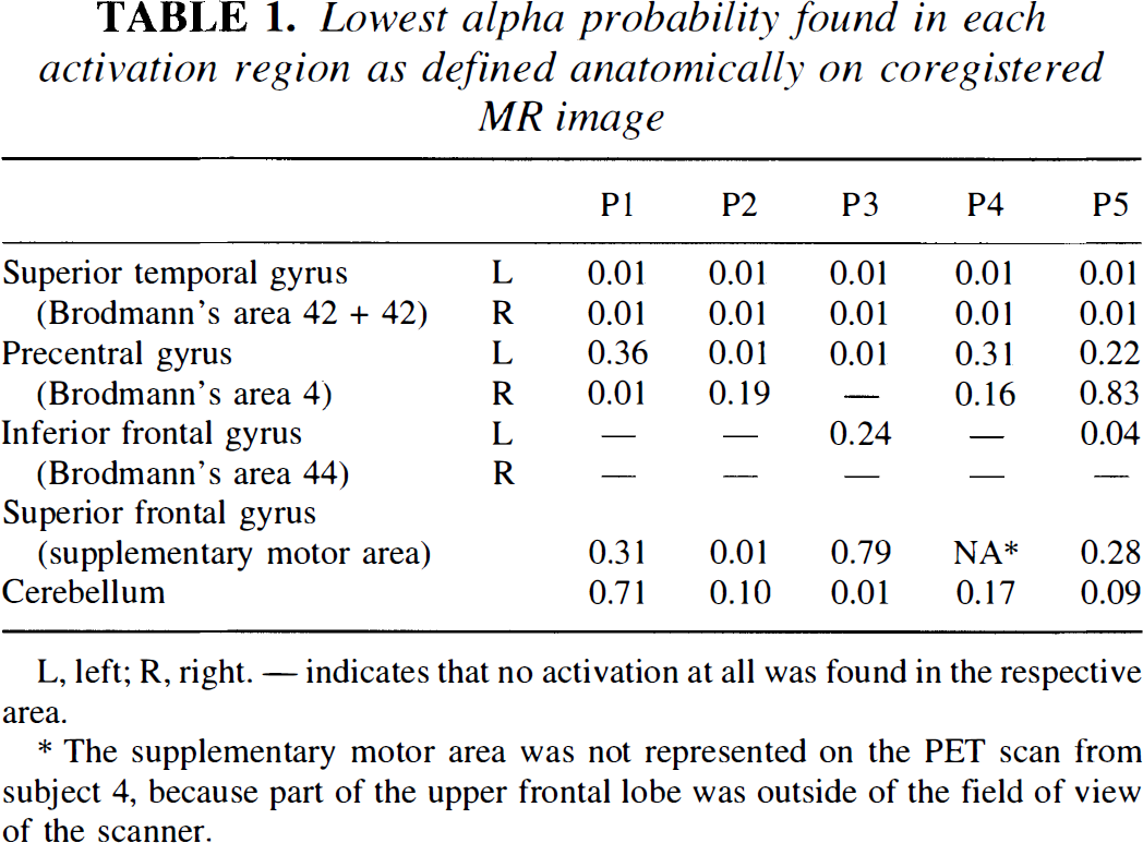
L, left; R, right. — indicates that no activation at all was found in the respective area.

*

The supplementary motor area was not represented on the PET scan from subject 4, because part of the upper frontal lobe was outside of the field of view of the scanner.

There was considerable variability of the location of the activation maximum along the anteroposterior axis of the superior temporal gyrus. As an extension to the description of cortical localization in terms of stereotactic coordinates, the projection of the activation foci onto the anatomical structure is shown in Figure 5 for these four patients for whom high-resolution magnetic resonance images were available. In every subject, the activated areas comprised the lateral parts of Brodmann's areas 41 (primary auditory cortex) and 42 (auditory association cortex), as well as parts of Brodmann's area 22 (on the convexity surface). To determine the amount of activation that was detected as being significant for each subject, the mean difference of the rest and activation voxels was calculated for all voxels whose associated a probability was less than 0.05 (Table 2). The smallest activation that could be detected had a CBF increase of 17.6% (subject P5). It comprised also the largest number of voxels. The smallest total activated volume was 132 voxels (1.9 cm³), with a CBF increase of 28.7% (subject P4).

Fig. 5.

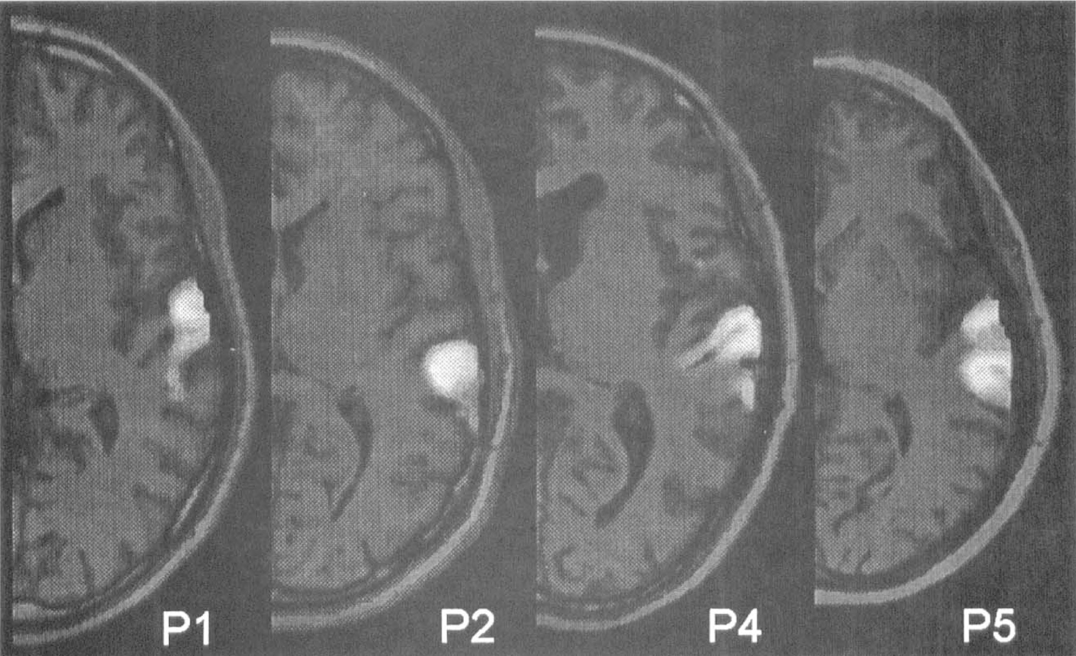
Probability map of the activation in the superior temporal gyrus represented in a gray scale from 1 (black) to 0 (white) and overlaid on the corresponding magnetic resonance imaging slice, showing the very good correspondence between activated area and gyral structure.

Table 2.

Activation quantification

		P1	P2	P3	P4	P5
P < 0.05	percent activation	20.8	21.8	24.0	28.7	17.6
	standard deviation	1.6	1.5	2.7	2.0	2.4
	number of voxels	181	222	592	132	838

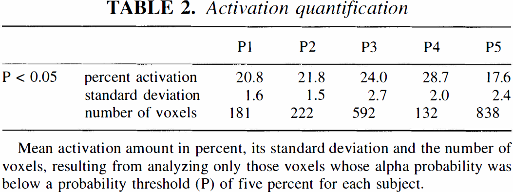
Mean activation amount in percent, its standard deviation and the number of voxels, resulting from analyzing only those voxels whose alpha probability was below a probability threshold (P) of five percent for each subject.

DISCUSSION

With increasing filter kernel size, the signal-to-noise ratio increases and the spatial resolution decreases. Therefore, the optimal size of the filter kernel varies with the desired spatial resolution and the noise properties of the images, which in turn can vary from subject to subject. A major component of total noise is caused by stochastic radioactive decay resulting in a Poisson noise distribution with variance proportional to the number of counts. Increasing the filter size is a very efficient way to increase the number of counts that contribute to each voxel, because the volume increases with the third power of filter FWHM. Increasing the injected dose only has a linear effect at best and in practice even less because the efficiency of the scanner decreases substantially at doses greater than the standard 370 MBq per injection. The computing time required for randomization tests also increases with the third power of the filter kernel radius for spherical filter kernels. Current calculation times of up to 30 minutes are still practical and will certainly be reduced by further computer hardware development. Larger filters can increase the area of significant response determined by randomization testing, while making impossible the exact localization of the activated area. Moreover, activation foci that can be distinguished clearly with finer filters may become indistinguishable with greater filters. In our experience, with Gaussian filters around 12-mm FWHM, reasonable numbers of activated voxels can be determined while preserving the spatial resolution necessary to map the activation foci to anatomic structures. Similar results could be obtained by using a spherical rather than Gaussian average filter, which showed reasonable activation detection properties around a 10-mm radius. The average filter is much more efficient in terms of computation time, because no weighting of voxel values is necessary, and may therefore be an option to perform the procedure on slower computers.

The term “repetition activation paradigm” was adapted from Petersen et al. (1988), except that the control condition was the resting state instead of passive presentation. As expected (Petersen and Fiez, 1993), we found activated areas in the superior temporal gyrus of both hemispheres, the primary sensorimotor mouth cortex, the supplementary motor area, and regions of the cerebellum. In all cases, in the left hemisphere the superior temporal activation extended to the posterior part of the superior temporal gyrus, indicating involvement of areas related to word comprehension and semantic processing, as proposed by Wise et al. (1991). Furthermore, the observed activation is very similar in location to the findings obtained with FDG-PET by Herholz et al. (1994).

Compared with the SPM results, activated areas are much more contiguous at the chosen level of significance. The randomization test is not susceptible to violations of the assumptions underlying parametric tests (Horwitz et al., 1995; Ford, 1995). It could therefore be considered a “gold standard” against which the parametric assumptions implicit in the use of SPMs could be tested (Friston, 1995). Some limitations still remain, namely the heavy dependence on details of the given procedural, sample-specific, imaging, and analysis conditions, which is reflected in our study as a heavy dependence on filter size.

The quantification of the activation by evaluating all significantly activated voxels revealed CBF increases around 20%. Cerebral blood flow increases of this magnitude are observed regularly only in primary sensory or motor areas, whereas typical activation effects in association areas that have been identified in group studies often did not exceed 10% or even 15%. It remains to be determined whether application of even larger filter sizes or usage of volumes of interest will improve the sensitivity of the procedure for studies of more complex higher brain functions. Sensitivity could also be improved if conditions that allow less variability of the cognitive state, in particular in the baseline condition, reduce CBF fluctuations within each condition.

It should be kept in mind that the spatial extent of the resulting activated voxel cluster at a given a threshold is valid only at the resolution imposed by the spatial filtering. Therefore, when projecting the activated voxels onto anatomic (e.g., magnetic resonance) images, the activation borders must be regarded with caution. Because the signal properties of the ¹⁵O-H₂O-scan are hard to model adequately (Ford, 1995), the probability of missing activated areas with this technique at a given type I error threshold, which represents the type II error, is very difficult to assess. Nevertheless, this would be important, for example, in preoperative speech cortex localization studies and therefore deserves further investigation.

In conclusion, we demonstrate the applicability of the randomization test method for single-case speech activation PET studies, evolving from sensitive (3D) scanner technology and high-speed computing devices. We consider single-case processing capability essential to the study of activation patterns in disease conditions like stroke, dementia, or brain tumors, in which brain anatomy is distorted and blood perfusion mechanisms are yet unknown, as possible therapeutic actions resulting from the localization of eloquent brain areas require evaluation procedures whose validity is guaranteed rather than assumed.