Nonparametric Analysis of Statistic Images from Functional Mapping Experiments

Abstract

The analysis of functional mapping experiments in positron emission tomography involves the formation of images displaying the values of a suitable statistic, summarising the evidence in the data for a particular effect at each voxel. These statistic images must then be scrutinised to locate regions showing statistically significant effects. The methods most commonly used are parametric, assuming a particular form of probability distribution for the voxel values in the statistic image. Scientific hypotheses, formulated in terms of parameters describing these distributions, are then tested on the basis of the assumptions. Images of statistics are usually considered as lattice representations of continuous random fields. These are more amenable to statistical analysis. There are various shortcomings associated with these methods of analysis. The many assumptions and approximations involved may not be true. The low numbers of subjects and scans, in typical experiments, lead to noisy statistic images with low degrees of freedom, which are not well approximated by continuous random fields. Thus, the methods are only approximately valid at best and are most suspect in single-subject studies. In contrast to the existing methods, we present a nonparametric approach to significance testing for statistic images from activation studies. Formal assumptions are replaced by a computationally expensive approach. In a simple rest-activation study, if there is really no activation effect, the labelling of the scans as “active” or “rest” is artificial, and a statistic image formed with some other labelling is as likely as the observed one. Thus, considering all possible relabellings, a p value can be computed for any suitable statistic describing the statistic image. Consideration of the maximal statistic leads to a simple nonparametric single-threshold test. This randomisation test relies only on minimal assumptions about the design of the experiment, is (almost) exact, with Type I error (almost) exactly that specified, and hence is always valid. The absence of distributional assumptions permits the consideration of a wide range of test statistics, for instance, “pseudo” t statistic images formed with smoothed variance images. The approach presented extends easily to other paradigms, permitting nonparametric analysis of most functional mapping experiments. When the assumptions of the parametric methods are true, these new nonparametric methods, at worst, provide for their validation. When the assumptions of the parametric methods are dubious, the nonparametric methods provide the only analysis that can be guaranteed valid and exact.

MOTIVATION

Functional mapping experiments using positron emission tomography (PET) and more recently magnetic resonance imaging produce data consisting of sets of three-dimensional images, with voxel values indicative of regional neuronal activity. The aim of simple activation studies is usually the identification of the brain regions that are affected by an experimental stimulus. In the absence of any prior knowledge regarding the location of these regions, the analysis usually proceeds at the voxel level.

Thus, images of statistics are formed, each voxel having associated with it the value of a simple statistic, expressing evidence of an activation at the corresponding brain location. These statistic images are sometimes called statistical parametric maps (SPMs). The challenge is to test these statistic images, assessing the omnibus significance of any activation at all, and localising reliably the regions that are activated.

Statistic images

Existing methods of analysis are based on the assumption of specific forms of probability distribution for the voxel values in the statistic images. Hypotheses are specified in terms of the parameters of the assumed distributions. Usually, scan data are taken to be normally distributed, giving known distributional forms for certain statistics.

Consider the simple paradigm where each of n subjects gives m images acquired under both rest and stimulation conditions. The simplest approach for this type of study is to construct an image of paired t statistics, based on subject mean difference images formed by subtracting the mean of the rest images from the mean of the activation images for each subject, after normalising each image by some measurement of global activity. (See Theory for details.) Under the hypothesis that all subject mean difference images have voxel values normally distributed with zero mean and unknown variance, the statistics at each voxel follow a Student t distribution with n − 1 degrees of freedom, giving a t statistic image.

Friston et al. (1990) proposed a completely randomised blocked design analysis of covariance (ANCOVA) for the analysis of multiple-subject activation studies. A simple linear model for the data is assumed, with voxel value expressed as a linear combination of subject effects (the block), scan effects, the global flow, and independent normally distributed errors of unknown variance. Evidence of an additive activation effect is expressed as a contrast of the scan effects, leading to a t statistic image with nm — n — m degrees of freedom. The degrees of freedom here are different from those of the paired t statistics already discussed, because the model assumptions are different. For moderately sized PET activation studies, the ANCOVA approach gives t statistic images with greater degrees of freedom, the assumptions being slightly stronger.

The voxel values in these statistic images will not be statistically independent. Neighbouring voxels have highly (positively) correlated values, because the reconstructed scan images are very smooth. In addition, there may be longer-range correlations due to biological relationships among separate brain regions.

Assessing statistic images

The most popular method for analysing these statistic images is to threshold them at a critical value. If no voxel statistic exceeds the threshold, then the omnibus hypothesis of no activation cannot be rejected. The hypothesis of no activation at individual voxels is rejected for voxels with suprathreshold statistics. The simplest methods are those derived from the inequalities due to Bonferroni and Sidák (see Westfall and Young, 1993, pp. 44–6). Each voxel statistic is tested individually at a significance level corrected to account for the number of voxels. If the voxel statistics are identically distributed, this gives a constant critical value at which to threshold the statistic image. These methods are very conservative when the tests are not independent, with actual Type I error probabilities (the size of the test) far below the target significance level of, say, 0.05.

Friston et al. (1991a) considered the smoothness of statistic images, to produce a less conservative test. Working in two dimensions, they considered a (nonactivated) statistic image, after probabilistic transformation to have a Gaussian distribution, as a good lattice representation of a continuous stationary isotropic Gaussian random field. Employing an argument based on the theory of level crossings in one-dimensional stochastic processes, they derived the approximate probability of a false positive at the pixel level, in terms of the threshold level and the smoothness of the statistic image. This is then used as the basis for a Bonferroni-like analysis.

Working independently, Worsley et al. (1992) considered (nonactivated) Gaussian statistic images as good lattice representations of homogeneous stationary Gaussian random fields, with zero mean and unit variance. With use of the work of Adler (1981) and A. M. Hasofer on the expected Euler characteristic of Gaussian random fields, the approximate probability that the maximum of such a field exceeds a given threshold was derived in terms of the volume under consideration and the smoothness of the field. Worsley's theory is sufficiently general to encompass the problem considered by Friston et al. (1991a). Worsley (1994) gives the expected Euler characteristic of χ², F, and t fields, enabling the approach to be used without forcing the consideration of Gaussian statistic images.

Shortcomings of existing methods

There are a number of problems with these random field approaches:

Low degrees of freedom. Statistic images are calculated using an estimate of the variance of the data (about the model under consideration) at each voxel. The low subject and scan numbers of PET studies result in variance estimates that are very variable, having χ²-distributions with low degrees of freedom (under assumptions of normality on image voxel values). This variability manifests itself as high (spatial) frequency noise in images of variance estimates, noise that is propagated through to statistic images. Continuous random t fields of low degrees of freedom are dominated by the variance field, as discussed by Worsley et al. (1993a), where it is demonstrated that a t field of 3 degrees of freedom almost surely becomes infinite at some point. For low degrees of freedom, >3, the variance field still dominates the t field, giving fields with features such as spikes smaller in spatial extent than the voxel dimensions, making untenable the consideration of a t statistic image as a lattice representation of a t field. This point is highlighted by Worsley et al. (1993b), in whose work critical thresholds for t statistic images with low degrees of freedom are obtained. These are much greater than those from a highly conservative Bonferroni correction. Current thinking is that t statistic images should be considered as good lattice representations of random t fields only if the degrees of freedom are at least 24. This casts doubt on the sensitivity of current parametric random field methods for the analysis of single-subject experiments.

Noisy statistic images. Even if the degrees of freedom are quite large, noise in statistic images can still be a problem. For a (continuous) random field to provide a reasonable approximation to a voxellated image, the smoothness of the image must be much greater than the voxel dimensions, but much less than the image dimensions. The estimated smoothness of noisy statistic images is low, and random fields of low smoothness may have features smaller in spatial extent than the voxel dimensions. Thus, random fields do not provide good approximations for noisy statistic images.

Pooled variance. To obtain smooth statistic images, well approximated by random fields, statistic images are either smoothed (after probabilistic transformation to have a Gaussian distribution under the null hypothesis) or computed using a constant global variance. The assumption of constant error variance, initially used by Worsley et al. (1992), has been criticised. [See discussion following Worsley et al. (1993), and that between Friston, Worsley, and Ford on pp. 671–3 of the same volume.] Reconstructed images, particularly from three-dimensional reconstructions, are more variable in the end planes than at the centre of the field of view. In addition to these physical factors are the physiological ones. Grey matter regions will have greater variance than ventricular regions. Further, differences in response to stimuli for different subjects would suggest that variance (in difference images) would be greater at the site of an activation. This appears to be so in activation experiments comparing two task conditions. A pooled variance estimate, in this case, underestimates the true regional variance at the activation site and therefore falsely inflates the statistic image there.

Statistic image smoothing. Smoothing trades spatial resolution for noise reduction, increasing the signal-to-noise ratio for signals greater in extent than the filter kernel. The effects are considerable, and different filtering algorithms can give radically different results. Thus, smoothing is undesirable when an activation is expected to be fairly localised or strong enough to be detectable. This secondary smoothing is not (in general) equivalent to smoothing the scan data.

Physical and physiological considerations would suggest that the error variance is spatially smooth, with the variance being constant for a small locality of voxels. This suggests the use of locally pooled variance estimates, formed by pooling variance estimates across neighbouring voxels, effectively smoothing the variance image. This would give smooth statistic images with no loss of resolution; the noise has been smoothed but not the signal. However, since neighbouring voxels have dependent values, the distribution of these locally pooled variance estimates is unknown. This precludes further analysis in a parametric manner.

Assumptions. In addition to these problems, existing methods rely on parametric assumptions, which are possibly false, and on various approximations, which may not be appropriate for the data at hand. In theory, assumptions can be checked. This is not routinely done in PET. In addition, the small data sets result in tests for departures from the assumptions with very low power. It is not known what effects departures from the assumptions have on the sensitivity and specificity of these complicated test methods. However, it should be noted that departures from assumptions will have the greatest effect on the tails of the assumed distributions for test statistics. We note that the tails of the distributions are of primary interest for the calculation of significance levels.

Nonparametric method

Thus, existing methods rely on a multitude of assumptions and approximations and restrict the form of the voxel statistic to those for which, distributional results are available. Having encountered problems with classic parametric methods when analysing EEG data, Blair and Karniski (1994) applied nonparametric methods. Originally expounded by Fisher (1935), Pitman (1937a,b), and later Edgington (1964, 1969a, 1980), these methods are receiving renewed interest as modern computing power makes the computations involved feasible. See Sprent (1993) for a modern text on nonparametric statistics and Edgington (1969a) for a thorough and readable exposition of randomisation tests.

Parametric methods make formal assumptions about the underlying probability model, up to the level of a set of unknown parameters. Scientific hypotheses formulated in terms of these parameters are then tested on the basis of the assumptions. In nonparametric methods, simple hypotheses about the mechanism generating the data are tested using minimal assumptions.

In the remainder of this article, we develop the theory for randomisation and permutation tests for functional mapping experiments. We shall concentrate on the simple activation experiment with a statistic image to be assessed using a single threshold. In Discussion we comment on this new method and explore its application to other experiments and the use of other statistics.

THEORY

The rationale behind randomisation and permutation tests is intuitive and easily understood. In a simple activation experiment, the scans are labelled as “rest” or “active,” and a statistic image is formed on the basis of these labels. If there is really no activation effect, then the labelling of the scans as “rest” or “active” is artificial, and any other labelling of the scans would lead to an equally plausible statistic image. Under the null hypothesis that the labelling is arbitrary, the observed statistic image is randomly chosen from the set of those formed from all possible relabellings. If each possible statistic image is summarised by a single statistic, then the probability of observing a statistic more extreme than a given value is simply the proportion of the possible statistic images with a statistic exceeding that value. Hence, p values can be computed and tests derived. In this section we formalise this heuristic argument, concentrating on randomisation tests where the probabilistic justification for the method comes from the initial random assignment of conditions to scan times.

Test validity

Formally, we have a family of hypotheses H_k of no activation at voxel k = (x,y,z). The omnibus null hypothesis H_Ω, of no activation anywhere in the brain, is true only if all the voxel hypotheses are true. Here Ω denotes the set of intracerebral voxels. Rejecting any voxel hypothesis implies rejection of the omnibus hypothesis and the declaration of that voxel as activated and the brain as activated somewhere. This is a multiple-comparison problem. We want to test the many voxel hypotheses individually whilst controlling the overall error rate.

For multiple-comparison problems, there are two forms of control of Type I error: weak and strong control (see Hochberg and Tamhane, 1987). Weak control merely requires that the omnibus test is valid. That is, the probability of declaring any voxel as activated when, in fact, none is, is at most a given level α, usually taken to be 0.05. A test with only weak control over Type I error can only declare a brain volume as “activated somewhere.” The test described by Friston et al. (1990) (known as the SPM “omnibus” test) is an example of a test that aims only for weak control over Type I error.

Strong control requires that, for any subset of the intracerebral voxels, the test of the omnibus hypothesis for this region is valid, even if the voxel null hypotheses are not true elsewhere. Strong control implies weak control. A test with strong control declares nonactivated voxels as activated with probability at most a, regardless of any true activation elsewhere, and therefore allows individual voxels to be reported as activated. The test has localising power.

Experiment

Consider a simple activation experiment with n subjects, each scanned repeatedly under two conditions denoted by A and B, with m repetitions of each condition.

The conditions are presented alternately to each individual. Half the subjects are randomly chosen to receive condition A first, then B, followed by m — 1) further A then B pairs (AB order, conditions presented ABAB…). The other half of the subjects receive condition B first (BA order, conditions presented BABA…). The randomisation of subjects to condition presentation order in this way protects against linear time effects confounding any condition effect in the statistic image.

After reconstruction, realignment, reshaping to a standard atlas, and any primary smoothing, the resulting preprocessed regional CBF (rCBF) images are then suitable raw data for computing statistic images.

Statistic images

For this article, we shall consider t statistic images, generalising to “pseudo” t statistics calculated using smoothed variance images. Changes in global CBF between scans must be accounted for by normalising rCBF. We adopt this approach because of its simplicity and because it illustrates some of the problems with statistic images with low degrees of freedom. Note that any reasonable method for producing statistic images, whose extreme values indicate activation, could equally well be used. In particular, more general modelling of the effect of global changes via ANCOVA is possible, at an increased computational burden.

Let A_jj(k) and B_ij(k) be the (preprocessed) CBF of subject i, i = 1, …, n; at repetition j, j = 1, …, m; at voxels with coordinates k = (x,y,z) ∈ Ω for the two conditions A and B, respectively. From these data, a set of n independent mean difference images Δ _i are constructed, one for each subject:

${\Delta }_i(k)=\frac{1}{m}\sum _{j=1}^m\left(\frac{B_{ij}(k)}{B_{ij}/50}-\frac{A_{ij}(k)}{A_{ij}/50}\right)$

(1)

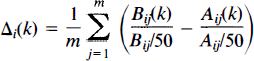
where Ā_ij and B̄_ij are the mean CBF computed over all intracerebral voxels. Hence, the images are individually normalised to have mean global CBF (gCBF)of 50 ml dl⁻¹ min⁻¹.

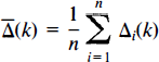
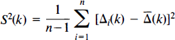
The mean and variance images for these data are estimated as Δ and S², respectively:

$\overline{\Delta }(k)=\frac{1}{n}\sum _{i=1}^n{\Delta }_i(k)$

(2)

$S^2(k)=\frac{1}{n-1}\sum _{i=1}^n{[{\Delta }_i(k)-\overline{\Delta }(k)]}^2$

(3)

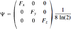
As discussed, we expect the true error variance to be smooth. Thus, consider a weighted locally pooled sample variance image S²_s obtained by convolving a Gaussian kernel of full width at half-maximum (FWHM) F_x × F_y × F_z mm with the voxel level sample variance image S²:

$S_s^2(k)=\frac{1}{\Sigma \varphi (k-k^{\prime })}\Sigma \varphi (k-k^{\prime })S^2(k^{\prime })$

(4)

$\varphi (x)=\frac{1}{{(2\pi )}^{3/2}\sqrt{\mid \Psi \mid }}exp(-\frac{1}{2}x{\Psi }^{-1}{x}^T)$

(5)

$\Psi =\left(\begin{array}{ccc}{F}_x& 0& 0\\ 0& F_y& 0\\ 0& 0& F_z\end{array}\right)\frac{1}{8\hspace{0.17em}ln(2)}$

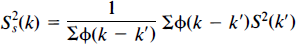
where φ is the filter kernel (Eq. 5). Summations are over the intracerebral voxels k′. In effect, the filter kernel is truncated at the edge of the intracerebral area, so edge effects are avoided. |Ψ| denotes the determinant of the matrix Ψ.

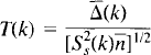
Using this smoothed sample variance in place of the voxel level variance in the formula for a t statistic gives us a pseudo t statistic image T:

$T(k)=\frac{\overline{\Delta }(k)}{{[S_s^2(k)\overline{n}]}^{1/2}}$

(6)

Null hypothesis and labellings

If the two conditions of the experiment affect the brain equally, then, for any particular scan, the acquired image would have been the same had the scan been acquired under the other condition. This leads to a suitable set of voxel hypotheses for no activation at each voxel: H_k—Each subject at each scan time would have given the same rCBF measurement at voxel k, were the conditions reversed.

The hypotheses relate to the data, which are regarded as fixed. Under the omnibus hypothesis H_Ω, any of the possible allocations of conditions to scan times would have given us the same scans. Only the labels of the scans as A and B would be different, and, under H_Ω, the labels of the scans as A or B are arbitrary. The possible labellings are those that could have arisen out of the initial randomisation. In this case, the possible labellings are those with half the subjects scans labelled in AB order and half BA order, giving N = _n C_n/2 = n!/[(n/2)!]² possibilities. Thus, under H_Ω, if we rerandomise the labels on the scans to correspond to another possible labelling, the statistic image computed on the basis of these labels is just as likely as the statistic image computed using the labelling of the experiment, because the initial randomisation could equally well have allocated this alternative labelling.

Randomisation distributions

For a simple threshold test, rejection or acceptance of the omnibus hypothesis is determined by the maximum value in the statistic image. The consideration of a maximal statistic deals with the multiple-comparison problem. Let T_max be the maximum of the observed statistic image T, searched over the intracerebral voxels; T_max = _max{T(k):k∈Ω}. It is the distribution of this maximal statistic that is of interest.

Under H_Ω, the statistic images corresponding to all N possible labellings are equally likely, so the maximal statistics of these images are also equally likely. Let tⁱ_max be the maximum value (searched over the intracerebral voxels values) of the statistic image computed for labelling i; i = 1, …, N. This set of statistics, each corresponding to a possible randomisation of the labels, we call the randomisation values for the maximal statistic. Then, when H_Ω is true, T_max is as likely as any of the randomisation values, because the corresponding labellings were equally likely to have been allocated in the initial random selection of labels for the experiment. This gives us the randomisation distribution of the maximal statistic, given the data and the assumption that H_Ω is true, as Pr(T_max = tⁱ_max|H_Ω) = 1/N (assuming that the tⁱ_max values are distinct).

Single-threshold test

From this, the probability (under H_Ω) of observing a statistic image with maximum intracerebral value as or more extreme than the observed value T_max is simply the proportion of randomisation values greater than or equal to it. This gives a p value for the omnibus null hypothesis.

This p value (for a one-sided test) will be <0.05 if T_max is in the largest 5% of the randomisation values, which it is if and only if it is greater than the 95th percentile of the randomisation values. Thus, for a test at level 0.05, a suitable critical value is this 95th percentile. This gives a test with weak control over Type I error at level 0.05: The probability of rejecting a true omnibus null hypothesis is the probability that any voxels in the observed statistic image have values exceeding the critical threshold. If any voxel values exceed the threshold, then the maximal one does, and the probability of this is at most 0.05 when the omnibus null hypothesis is true.

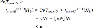
In general, for a level a test, the critical value is chosen as the 100(1 − α)st percentile of the randomisation values for the maximal statistic. Specifically, choose c as ⌊αN⌋, αN rounded down. The appropriate critical value is then the (c + 1)st largest of the tⁱ_max, which we denote by t^{(c + 1)}_max. The observed statistic image is then thresholded, declaring as activated those voxels with value strictly greater than the critical value. There are c randomisation values greater than t^{(c + 1)}_max (less if t^{(c + 1)}_max = t^(c)_max), so the probability of Type I error is

$Pr(T_{max}>t_{max}^{(c+1)}\mid H_{\Omega })\le c/N=\lfloor \alpha N\rfloor /N\le \alpha$

(7)

with equality if there are no ties in the sampling distribution and αN is an integer. Ties occur with probability zero for the maxima of statistic images from continuous data. The size of the test is less than 1/N smaller than α, depending on the rounding of αN. Weak control over Type I error is maintained. Thus, the test is (almost) exact, with size (almost) equal to the given level α. It can also be shown that the threshold test, with critical value as defined, has strong control over Type I error. The proof is given in Appendix.

Two-sided test

For a two-sided test, to detect activation and deactivation, the image of the absolute values of the statistics is thresholded. The randomisation distribution for the maximal absolute intracerebral value in the statistic image is computed exactly as shown, with maximum value replaced by maximum absolute value. For every possible labelling, the exact opposite labelling is also possible, giving statistic images that are the negatives of each other, and hence the same absolute maximum intracerebral value. Thus, the randomisation values are tied in pairs, effectively halving the number of possible randomisation values.

Single-step adjusted p value image

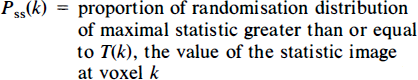
The p value for the observed maximal statistic has already been derived. For any other voxel, a p value can be computed as the proportion of the randomisation values, for the maximal statistic, greater than or equal to the voxel's value. These p values are known as single-step adjusted p values (Westfall and Young, 1993), giving a single-step adjusted p value image P_ss for these data:

$\begin{array}{lll}{P}_{\text{ss}}(k)\hfill & =\hfill & \text{proportion}\hspace{0.17em}\text{of}\hspace{0.17em}\text{randomisation}\hspace{0.17em}\text{distribution}\hfill \\ \hfill & \hfill & \text{of}\hspace{0.17em}\text{maximal}\hspace{0.17em}\text{statistic}\hspace{0.17em}\text{greater}\hspace{0.17em}\text{than}\hspace{0.17em}\text{or}\hspace{0.17em}\text{equal}\hfill \\ \hfill & \hfill & \text{to}\hspace{0.17em}T(k),\hspace{0.17em}\text{the}\hspace{0.17em}\text{value}\hspace{0.17em}\text{of}\hspace{0.17em}\text{the}\hspace{0.17em}\text{statistic}\hspace{0.17em}\text{image}\hfill \\ \hfill & \hfill & \text{at}\hspace{0.17em}\text{voxel}\hspace{0.17em}k\hfill \end{array}$

(8)

For a test at level α, this adjusted p value image is thresholded at level α, declaring voxels with adjusted p values less than or equal to α as activated.

A voxel with associated p value less than (or equal to) α must have value exceeded (or equalled) by at most αN members of the randomisation distribution of the maximal statistic, from the definition of the adjusted p values. There are c + 1 members of the randomisation distribution of the maximal statistic greater than or equal to the critical threshold t^{(c + 1)}_max, and, since c + 1 = ⌊αN⌋ + 1 > N, the voxel's value must exceed the critical threshold. Similarly, a voxel with value exceeding the critical threshold is itself exceeded or equalled by at most c members of the sampling distribution of the maximal statistic, and therefore has an adjusted p value at most α. Hence, thresholding the single-step adjusted p value image at a is equivalent to this test thresholding the observed statistic image at the 100(1 — α)th percentile of the randomisation values of the maximal statistic.

Secondary activation conservativeness

So far, we have been considering single-threshold tests, a single-step method in the language of multiple comparisons (Hochberg and Tamhane, 1987). The critical value is obtained from the randomisation distribution of the maximal statistic over the whole intracerebral volume, either directly or via adjusted p value images. It is somewhat disconcerting that all voxel values are compared with the distribution of the maximal one. Should not only the observed maximal statistic be compared with this distribution?

An additional cause for concern is the observation that an activation that dominates the statistic image will raise the observed maximal statistic above what it might be, were there no activation. Such a strong activation will influence the statistic images for the relabellings, particularly those for which the labelling is close to that of the experiment, possibly dominating the relabelled statistic image and hence leading to higher randomisation values than were there no activation. Thus, strong activation can increase the critical value of the test. This does not affect the validity of the test, but makes the test more conservative for voxels other than that with maximum observed statistic, as indicated by Eq. 9 in the proof of strong control for the threshold test. In particular, the test would be less powerful for a secondary activation in the presence of a large primary activation than for the secondary activation alone. Should not regions identified as activated be disregarded, and the sampling distribution for the maximal statistic over the remaining region used?

We now consider step-down tests, extensions of the single-step procedures. These are designed to address the issues raised and are likely to be more powerful.

Step-down test

The step-down test described here is a sequentially rejective test (see Holm, 1979), adapted to the current application of randomisation testing. Starting with the intracerebral voxels, the p value for the maximal statistic is computed as described. If this p value is greater than α, the omnibus hypothesis is accepted. Otherwise, the voxel with maximum statistic is declared as activated and the test is repeated on the remaining voxels, possibly rejecting the null hypotheses for the voxel with maximal value in this reduced set of voxels. This is repeated until a test rejects no further voxel hypothesis, at which stage the sequence of tests stops. Thus, activated voxels are identified, cut out, and the remainder of the volume of interest analysed, the process iterating until no more activated voxels are found.

The algorithm is as follows:

Algorithm a

1. Let w be the number of intracerebral voxels, and let k₁, …, k_w be the intracerebral voxels ordered such that their values in the observed statistic image go from smallest to largest. That is, T(k_w) is the maximal intracerebral value, and T(k₁) is the minimum. (Voxels with tied values may be ordered arbitrarily.)

2. Set i = w.

3. Compute the sampling distribution of the maximal value of the statistic image searched over the set of voxels {k₁, …, k_i,}.

4. Compute the p value P′_sd(k_i) as the proportion, of the sampling distribution just computed, greater than or equal to T(k_t).

5. If P′_sd(k_i) is less than or equal to α, then H_k can be rejected: Set r = i, decrease i by 1, and return to step 3. If H_ki cannot be rejected or there are no more voxels to test, then continue.

6. Reject H_k for k = k_r, …, k_w.

7. The corresponding threshold is the (c + 1)st largest member of the last sampling distribution calculated, for c = ⌊αN⌋, as above.

The test proceeds one voxel per step, from the one with largest intracerebral value in the observed statistic image, down to that with the smallest value.

This defines a protected sequence of tests, in that each test “protects” those following it, as each test must reject the omnibus null hypothesis for the remaining region to proceed to subsequent tests. In particular, the first test protects the entire sequence. This first test is simply the randomisation test of the overall omnibus hypothesis. Therefore, the multistep test has weak control over Type I error. Strong control is also maintained, the proof being left to Appendix.

An adjusted p value image, corresponding to the test, is computed by enforcing monotonicity of the p values computed in step 4, so that once the adjusted p value exceeds α, no further voxels are declared significant. This adds a further step to the algorithm:

• 8.

  Enforce monotonicity of the adjusted p values:

  $\begin{array}{lll}\hspace{0.17em}\hspace{0.17em}\hspace{0.17em}\hspace{0.17em}{P}_{\text{sd}}(k_w)\hfill & =\hfill & P_{\text{sd}}^{\prime }(k_w)\hfill \\ P_{\text{sd}}(k_{w-1})\hfill & =\hfill & max[P_{\text{sd}}(k_w),P_{\text{sd}}^{\prime }(k_{w-1})]\hfill \\ P_{\text{sd}}(k_{w-2})\hfill & =\hfill & max[P_{\text{sd}}(k_{w-1}),P_{\text{sd}}^{\prime }(k_{w-2})]\hfill \\ \hspace{0.17em}\hspace{0.17em}\hspace{0.17em}\hspace{0.17em}\hspace{0.17em}{P}_{\text{sd}}(k_r)\hfill & =\hfill & max[P_{\text{sd}}(k_{r+1}),P_{\text{sd}}^{\prime }(k_r)]\hfill \\ \hspace{0.17em}\hspace{0.17em}\hspace{0.17em}\hspace{0.17em}\hspace{0.17em}{P}_{\text{sd}}(k_1)\hfill & =\hfill & max[P_{\text{sd}}(k_2),P_{\text{sd}}^{\prime }(k_1)]\hfill \end{array}$

Note that it will only be possible to compute these adjusted p values for the voxels for which P′_sd(k_i) were computed, voxels with significant statistics at level α. One particular advantage of forming the full adjusted p value image here is that the test level does not need to be specified in advance of computations. Voxels declared activated by the step-down test are precisely those with adjusted p value less than or equal to α.

In this form, the test is too computationally intensive to be useful, involving the computation of a new randomisation distribution for each step. It is possible to accelerate the test, using the single-threshold test at each step to identify activated voxels and exclude them en masse in the next step, rather than considering only the voxel with maximal statistic at each step. This “step-down in jumps” variant provides a computationally feasible equivalent test. A more efficient approach to the step-down test is to accumulate the proportions for the adjusted p values, P′_sd(k), for all voxels simultaneously as each relabelled statistic image is computed. Due to Westfall and Young (1993), this method gives only adjusted p value images. The algorithm is as follows:

Algorithm b

1. As above.

2. Initialise counting variables C_i = 0; i = 1, …, w. Let j = 1.

3. Generate the statistic image t^j corresponding to possible labelling j.

4. Form the successive maxima:

   $\begin{array}{lll}{v}_1\hfill & =\hfill & t^j(k_1)\hfill \\ v_2\hfill & =\hfill & max[v_1,t^j(k_2)]\hfill \\ v_3\hfill & =\hfill & max[v_2,t^j(k_3)]\hfill \\ \hfill & \hfill & :\hfill \\ v_w\hfill & =\hfill & max[v_{w-1},t^j(k_w)]\hfill \end{array}$

5. If v_i ≥ T(k_i), then increment C_i by 1.

6. Repeat steps 3–5 for each remaining possible relabelling j = 2, …, N.

7. Compute p values P′_sd(k_i) = C_i/N.

8. As above, (monotonicity enforcement).

Each step of the step-down algorithm (algorithm a) computes the p value P′_sd(k_i) as the proportion of the randomisation values for the maximal statistic that are greater than T(k_i), where the maximal statistic is searched for over voxels {k₁, …, K_i}, the i voxels whose hypotheses have not yet been assessed. In algorithm b, for each possible labelling, v_i is the maximum of the statistic image corresponding to the labelling, searched over voxels {k₁, …, k_i}. Thus, it is clear that algorithm b accumulates the proportions for the adjusted p values as each relabelled statistic image is computed, giving the same adjusted p values as algorithm a.

EXAMPLE APPLICATION

Data acquisition and preparation

The PET experiment analysed with the randomisation procedures developed herein is the simple two-condition activation study published by Watson et al. (1993), to which the reader is referred for comprehensive details of the experiment.

In brief, 12 subjects underwent 12 sequential scans in a single session. With use of an H₂¹⁵O infusion, images of relative rCBF were acquired under two stimulation conditions. During condition A scans, subjects viewed a random stationary pattern of small squares. For condition B, the squares moved smoothly in random directions. The conditions were presented alternately, the series commencing with A in six randomly chosen subjects and B for the remaining six. The aim of the study was to identify area V5, the motion centre of the visual cortex.

Data were acquired on a CTI 953B PET tomograph with septa retracted, corrected for attenuation, and reconstructed by three-dimensional filtered back-projection giving images with resolution 8.5 × 8.5 × 4.3 mm at FWHM. Images were realigned within each subject. The brain was identified by reference to coregistered magnetic resonance images, and other areas removed from the images. The resulting images were transformed to the stereotactic atlas of Talairach and Tournoux, using the methods of Friston et al. (1989, 1991b). Finally, images were smoothed by convolution with a Gaussian kernel of FWHM 10 × 10 × 12 mm to overcome residual anatomical variability, leading to smoothed images with approximately isotropic resolution.

Statistic images

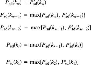
Study mean difference image and local statistics. The study mean difference image A is very smooth and the VI and V5 areas are clearly visible (Fig. 1a). The sample variance image S², however, is quite noisy, being computed from only 12 subjects.. It is also clearly not flat, showing increased variance of mean difference in response to the two conditions in the visual cortex (Fig. 1b). Thus, it is unreasonable to assume that the variance is constant over the intracerebral volume. The noise is propagated to the t statistic image (Fig. 1c). Due to the relatively large subject numbers (n = 12, 11 degrees of freedom), the noise here is not as extreme as can be seen with smaller studies, but it is still sufficiently variable to warrant using a locally pooled sample variance estimate.

FIG. 1.

a: Mesh plot for the intercommissural [anterior-posterior commissural (AC-PC); z = 0] plane of the observed study mean difference image Δ. The x and y coordinates are in Talairach space, so the x-axis runs from left to right and the y-axis from front to back with the posterior of the brain at y = −100. The heights of the vertices of the mesh indicate the value of Δ for each voxel, z-axis label: Δ (k)/(ml dl⁻¹ min^-1), b: Mesh plot for AC-PC plane of observed voxel level sample variance S². z-axis label: S²(k)/(ml dl⁻¹ min⁻¹)², c: Mesh plot for AC-PC plane of observed t statistic image computed with voxel level variance estimates, z-axis label: t statistic.

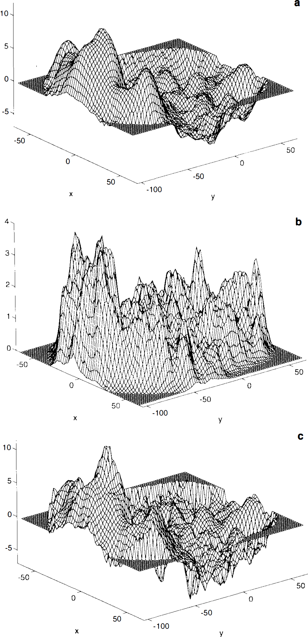
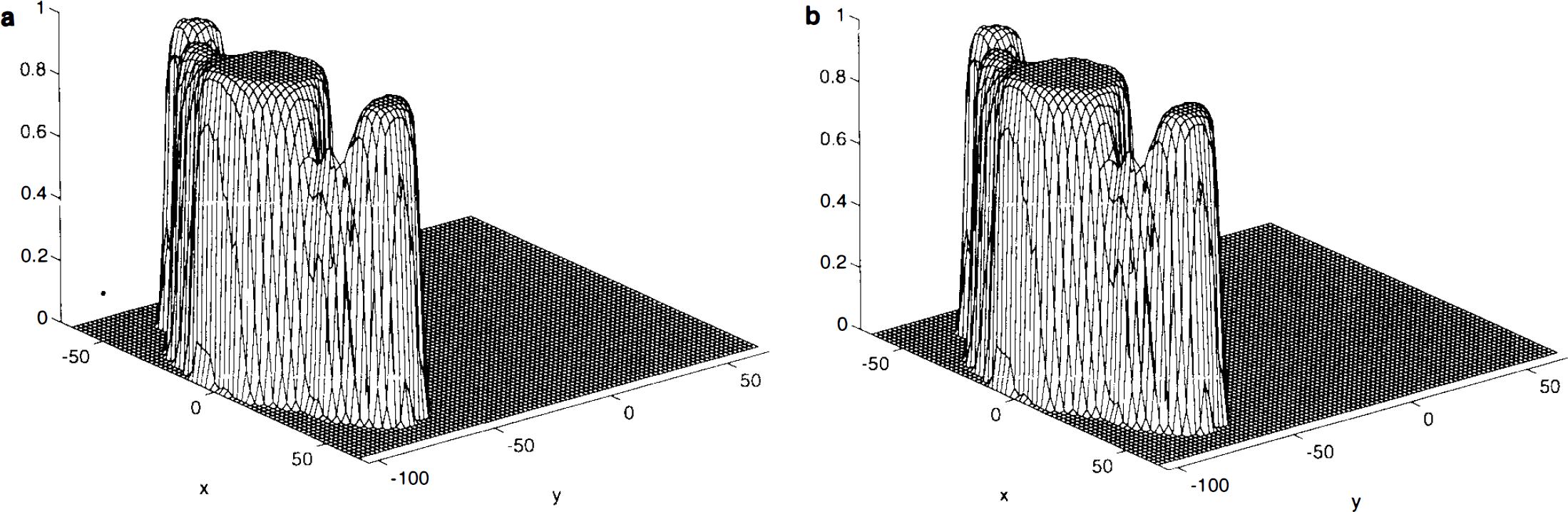
Smoothed sample variance and pseudo t-statistic. The weighted locally pooled sample variance estimate S² _s was obtained by smoothing the sample variance image with a Gaussian kernel of FWHM 10 × 10 × 6 mm. The filter size was arbitrarily chosen to be just less than the resolution of the preprocessed images, but reduced in the z-direction to avoid excessive edge effects. (The appropriate choice of filter for computing these weighted locally pooled variance estimates remains to be investigated.) The resulting sample variance image is smooth (Fig. 2a), but has the large-scale structure of the sample variance image without the noise. The resolution conforms to what would be expected given the scanner resolution and other physical and physiological conditions. The resulting pseudo t statistic image is much more appealing than the t statistic image (Fig. 2b), the noise having been smoothed.

FIG. 2.

a: Mesh plot for anterior-posterior commissural (AC-PC) plane of smoothed sample variance estimate S²_z. z-axis label: S²_z(k)/(ml dl⁻¹ min⁻¹)², b: Mesh plot for AC-PC plane of pseudo observed t statistic image computed with smoothed sample variance estimate. The noise has been smoothed but the signal has not been altered, z-axis label: T(k)/(ml dl⁻¹ min⁻¹)².

Randomisation tests

Relabelling. For this design there are N = ₁₂C₆ = 924 possible relabellings of the labels on the scans, each allocating six subjects to AB order and six to BA order. The possible labellings partition into two halves, as for each possible labelling the exact opposite is possible also. Given a particular labelling and the resulting statistic image, the opposite labelling gives the negative of the statistic image. Thus, it is necessary only to compute statistic images corresponding to half the possible labellings, the remainder being obtained as their negatives.

Randomisation values. For each possible labelling, the corresponding statistic image was computed and the maximum intracerebral value retained. These randomisation values (Fig. 3a) for the maximal statistic are all equally likely under H_Ω. Computations in MatLab on a Sun Sparc2 took ∼14 h, including the smoothing of the 462 variance images. Without this smoothing, computation takes ∼8h.

FIG. 3.

a: Histogram of the randomisation distribution for the maximal intracerebral voxel for these data, computed over all 924 possible randomisations of the labels of the scans. The statistic corresponding to the actual labelling of the experiment is the largest one, at T_max ≈ 12.34. x-axis label: t_max/Ω; y-axis label: frequency, b: Voxels with observed pseudo t statistic exceeding the critical threshold, computed from the randomisation distribution, the null hypotheses for these voxels can be rejected at experimentwise error level α = 0.05. The brain outline is also shown. The first slice shown (top left) is plane 3 [anterior–posterior commissure (AC-PC) −20 mm], the sixth is plane 8 (AC-PC), and the last plane (bottom right) is plane 23 (AC-PC +20 mm), successive planes spaced by 4 mm. Planes are oriented with the front right of the brain at the top right of the picture. The primary visual cortex (V1) is the large midline activated area towards the rear of the brain; the two satellite activations on planes 4–8 correspond to the motion centre (V5).

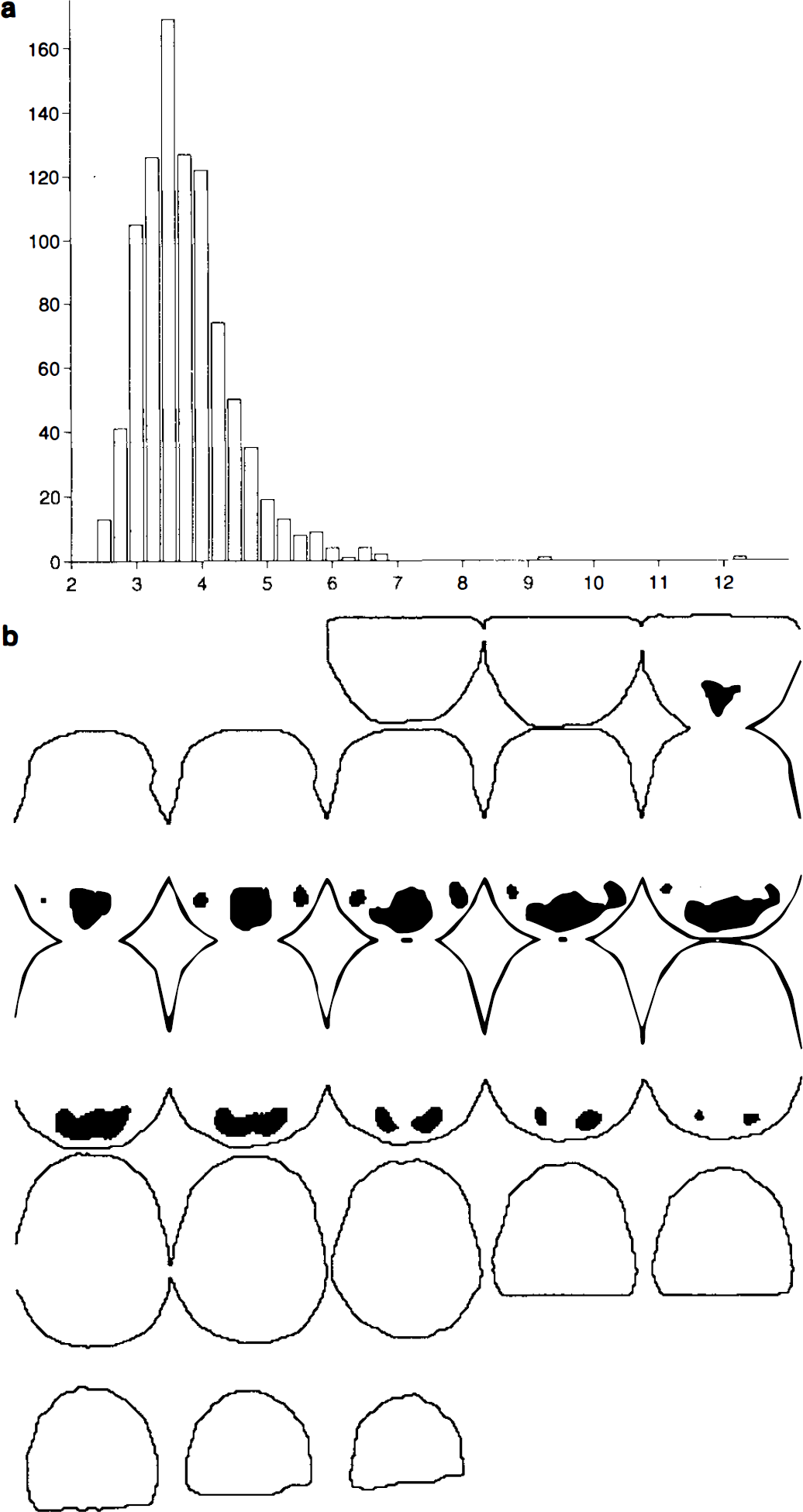
Omnibus test. The maximum statistic in the pseudo t statistic image (formed with labels as in the actual experiment) was the largest in the sampling distribution, so a p value for the omnibus null hypothesis, that the scans would have been the same whatever the condition, is 1/924, indicating significant evidence against this hypothesis.

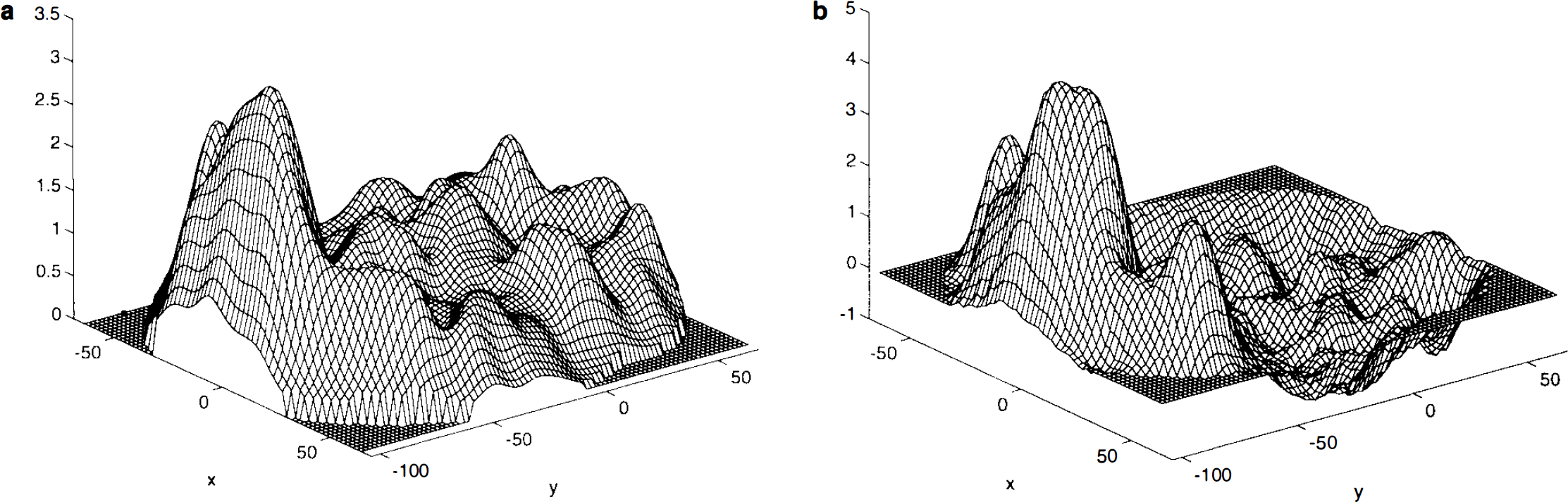
Single-threshold test. For a level α = 0.05 test, the appropriate critical value is the c = ⌊αN⌋ + 1 = 47th largest randomisation value of the maximal statistic, t⁽⁴⁷⁾_max = 5.083 (to three decimal places). Values of the observed pseudo t statistic image greater than this threshold indicate significant evidence against the corresponding voxel null hypothesis, at the 5% level (Fig. 3b). The locations of these 2,779 voxels in Talairach space can be declared as the activation region. There is a large primary activation in the V1 area, with lesser secondary activation in the V5 areas to either side. The single-step adjusted p value image shows the significance of the activation at each voxel (Fig. 4a).

FIG. 4.

a: Single-step adjusted p value image. The smaller the p value, the greater the evidence of activation. To aid visualisation, the p values are displayed subtracted from 1, with the background set to 0. Voxels with p value less than (or equal to) α indicate activation at significance level α, for any experimentwise error level α. z-axis label: 1 — P_ss. b: Step-down adjusted p value image, z-axis label: 1 — P_sd.

It is interesting to note that the rejected region is slightly larger than in the analysis of Watson et al. (1993) who used ANCOVA and the two-dimensional analysis of Friston et al. (1991a). The latter was applied plane by plane with no correction for the number of planes under consideration. An analysis of the t statistic image (computed with local variance), using the method of Worsley et al. (1992), adapted for t fields on 11 degrees of freedom using the appropriate expected Euler characteristic (Worsley, 1994), picks out only a small number of voxels in the V1 area.

Step-down methods. The step-down test gave a critical threshold of 5.0393 (to 4 decimal places), after four steps of the “step-down in jumps” modification of the step-down algorithm, the steps picking out 2,779, 37, 9, and 0 activated voxels. Thresholding the observed statistic image at this level gives 2,825 voxels being declared as activated, a mere 46 more than with the single-threshold test. The recommended way to apply the step-down test is via adjusted p value images computed directly. Computation took 24 h, including formation of the statistic images, involving variance smoothing. The step-down adjusted p value image (Fig. 4b) is almost the same as the single-step adjusted p value image (Fig. 4a). The improvement in sensitivity of the step-down method over the single-threshold method is minor for these data, even though there is a large signal. In this example, the single-threshold test is adequate, and the step-down test is probably not worth the computational effort involved.

DISCUSSION

Permutation tests

We have been considering a randomisation test for a particular activation study, where the only assumption is that of an initial random assignment of conditions to subjects. This assumption gives a random element to the experiment, permitting hypothesis testing. It replaces the assumption of parametric analyses, that the scans are sampled from some population of known form. However, these nonparametric methods are not limited to experiments where there was an initial randomisation. Permutation tests are computationally the same as the randomisation tests presented herein, but the justification for relabelling and computing randomisation distributions comes from weak distributional assumptions. For the simple activation study experiment, assume that for each voxel k the values of the subject mean difference images are drawn from a symmetric distribution centered at μ _k . Under H_k:μ _k = 0, the subject mean difference image at k is as likely as its negative, corresponding to the opposite labelling of the subject's scans. Thus, under H_Ω, the 2 _n statistics images, corresponding to all possible labellings of the subjects scans as A or B, are equally likely. However, as six subjects were given the opposite condition presentation order to protect against detecting time effects, only the _n C_n/2 permutations of the labels retaining this balance should be considered (Hochberg and Tamhane, 1987, p. 267), giving the same test as the randomisation approach. Indeed, many authors neglect the theoretical distinction between randomisation tests and permutation tests and refer to both as permutation tests. The advantage of the randomisation test over the permutation test, with its implicit weak distributional assumptions, is that the random allocation assumption of the former is clearly true, yielding a valid test.

Other applications

These nonparametric methods can be applied to many paradigms in functional neuroimaging. For statistic images, where large values indicate evidence against the null hypothesis, we have developed the theory for a single-threshold test and a step-down extension. All that is required is a concept of a label for the data, on the basis of which a statistic image can be computed, and a null hypothesis specified. Region-of-interest or parallel group designs, comparing (for instance) a control group with a disease group, can be easily accommodated. Indeed, a randomisation alternative is available for most experimental designs. See Edgington (1980) for a thorough exposition. Consider the following examples:

Single-subject correlation. It is wished to locate the regions of an individual's brain in which activity increases linearly with the difficulty of a certain task. During each of m scans, the subject is given the task at a given level of difficulty, the order of presentation having been randomly chosen from the m! possible allocations. The evidence for linear association of rCBF and difficulty level at a given voxel may be summarised by the correlation of rCBF (after some form of global flow correction) and difficulty level or indeed by any suitable statistic. The “labels” here are the actual task difficulty levels. Under the null hypotheses H_Ω:[the individual would have had the same rCBF whatever the task difficulty], the statistic images corresponding to all m! possible randomisations of the task difficulties are equally likely, and a randomisation test follows as described.

Single-subject activation experiment. It is wished to locate the region of an individual's brain that is activated by a given task, over a given baseline condition. The subject is scanned an even number of times, with the conditions applied in pairs, giving m/2 successive rest–activation pairs. The order of the conditions within each pair of scans is randomly chosen.

A statistic image is formed whose large values indicate evidence of an increase in rCBF between the baseline and activation condition. Under H_Ω: [each scan would have given the same rCBF image had it been acquired under the other condition], statistic images formed by permuting the labels within individual pairs of scans are as likely as that observed. Thus, the labels here are the scan condition, “baseline” or “activation,” and the possible labellings are those for which each successive pair of scans are labelled AB or BA. There are m/2 such pairs, so the randomisation distribution of the statistic image will consist of 2^m/2 images.

Other statistics

As we have seen, these nonparametric tests can be applied to any form of statistic image, unlike parametric analyses, where the choice of statistic is limited to those of known distributional form (for suitable assumptions on the data). This enables the consideration of the pseudo t statistic image formed with a smoothed variance estimate, for which no distributional results are available. This gives the researcher a free hand to invent experimental designs and devise statistics. However, it is advisable to use a standard experimental design and standard test statistic, if these exist, possibly modifying the statistic to take advantage of the image setting, for example, by smoothing. Standard test statistics are usually those that give the most powerful test in the parametric setting, when the assumptions are true, and can therefore be expected to remain sensitive statistics when the assumptions are slightly in doubt.

The application of these randomisation and permutation tests is also not limited to the single-threshold and step-down tests discussed. The procedure gives the randomisation distribution of the whole statistic image, and hence of any statistic summarising an image.

By computing the proportion of voxels with statistic exceeding a given threshold, for each of the statistic images in the randomisation distribution, a nonparametric version of the omnibus test proposed by Friston et al. (1990) could be obtained.

Cluster threshold tests

Recent work has concentrated on assessing the significance of possible signals by their spatial extent rather than their maximum amplitude. These techniques threshold the statistic image at a relatively low level, obtaining clusters of suprathreshold voxels. Clusters greater than a given critical size are declared as “activated.”

To find the critical cluster size for a size α test for various thresholds, Poline et al. (1993) and Roland et al. (1993) estimated the null distributions of suprathreshold cluster size by simulation, generating statistic images with variance and (homogeneous) smoothness matching those of rest–rest comparisons from activation studies. The match between the simulated data and a real null statistic image from a future experiment is questionable, and the sensitivity of the critical values to variations from the simulated parameters is not known. Furthermore, in the two studies referenced here, there are further approximations and assumptions. Thus, the critical values obtained give only approximately valid tests.

Friston et al. (1994) apply the theory of excursion sets in continuous random fields (Adler, 1981) to derive an equation, giving the approximate probability of observing a cluster greater than a given size, in a Gaussian random field of given smoothness, thresholded at a given level. Setting this equal to α and solving gives the critical suprathreshold cluster size for a test with approximate size α. Amongst other assumptions, the theory relies on the image being well approximated by a continuous random field, and so is subject to the same problems with noisy statistic images as the single-threshold approach of Worsley et al. (1992).

If images are summarised by the size of the largest cluster of voxels with values above a given threshold, then computing this for the statistic images corresponding to each of the possible labellings gives the randomisation values for maximal suprathreshold cluster size. These randomisation values can then be used as those for the maximal voxel statistic were in the theory described, to give a critical cluster size, above which the (omnibus) null hypothesis for the voxels in the cluster can be rejected at significance level α. Strong control follows on a cluster-by-cluster basis. (Individual voxel hypotheses are not tested individually in these cluster threshold tests.) Thus, nonparametric cluster threshold tests are possible.

Number of possible labellings, size, and power

A key issue for randomisation and permutation tests is the number N of possible labellings, as this dictates the number of observations from which the sampling distribution is formed. For the possibility of rejecting a null hypothesis at the 0.05 level, there must be at least 20 possible labellings, in which case the observed labelling must give the most extreme statistic for significance. Since the observed statistic is always one of the randomisation values, the smallest p value that can be obtained from these methods is 1/N. This is illustrated in the adjusted p value images of Fig. 4, where the smallest possible p value of 1/924 is attained for most of the activated region, although the observed pseudo t statistic image has a clear maximum. So, to demonstrate stronger evidence against the null hypothesis, via smaller p values, larger numbers of permutations are required. As the possible labellings are determined by the design of the experiment, this limits the application of nonparametric tests to designs with moderate subject and/or scan per subject numbers. The single-subject activation experiment described has only 2^m/2 possible labellings, 64 for a 12-scan session or 128 for a 14-scan session. The greater N, the greater the power, as this implies more data.

As N tends to infinity, the sampling distribution tends to the distribution of the test statistic for a parametric analysis, under suitable assumptions (Hoeffding, 1952). Thus, if all the assumptions of a parametric analysis are correct, the sampling distribution computed from a large number of relabellings is close to the hypothetical (parametric) distribution of the test statistic, were data randomly sampled from an appropriate model. For smaller N, nonparametric methods are, in general, not as powerful as parametric methods when the assumptions of the latter are true. In a sense, assumptions provide extra information to the parametric tests, giving them the edge. The attraction of the nonparametric methods is that they give valid tests when assumptions are dubious, when distributional results are not available, or when only approximate theory is available for a parametric test.

Approximate tests

In many cases the number of possible labellings is very large, and the computation involved makes it impractical to compute of all the randomisation values. For instance, the single-subject correlation study described has m! possible labellings, 479,001,600 for a 12-scan experiment. Here, approximate tests can be used (Edgington, 1969b). Rather than compute all the randomisation values, an approximate randomisation distribution is computed using a subject of the possible labelings. The subset consists of the true labelling and N′ − 1 randomly chosen from the set of possible relabellings (usually without replacement). The tests then proceed as before, using this subset of the randomisation values. A common choice for N′ is 1,000, so the randomisation values are those formed with the observed labelling and 999 relabellings chosen randomly from the set of those possible.

Despite the name, the approximate tests are still (almost) exact; only the randomisation distribution is approximated. The randomisation values used can be thought of as a random sample of size N′, taken from the full set of randomisation values, one of which corresponds to the observed labelling. Under the null hypothesis, all the members of the subset of randomisation values are equally likely, so the theory develops as before. As the critical threshold is estimated, it has some variability about the true value that would be obtained from the full set of randomisation values. This results in a loss of power, but the loss is very small for approximate sampling distributions of size 1,000. See Edgington (1969a,b) for a full discussion.

Conservativeness of one-sided tests in presence of large decreases

The possibility of a large activation causing these tests to be conservative for a secondary activation has been discussed. A similar difficulty arises for one-sided tests, when there are strong negative signals or deactivations. As noted, for each possible labelling in the activation experiment, the opposite labelling is also possible. In labellings that are almost completely the opposite of the actual labelling of the experiment, these negative signals will appear as positive signals. Thus, strong negative signals can inflate the critical threshold, making the test conservative for positive signals. These strong negative signals would not be “cut out” by a one-sided step-down test. One remedy for this problem could be to consider a two-sided step-down test. However, for the V5 data presented here, such an approach affords no improvement.

There remains the issue of whether a deactivation is real or an artefact of global normalisation. If gCBF (measured as the global mean) remains constant, then any local increase in rCBF must be accompanied by a decrease in rCBF elsewhere. If there is an increase in rCBF but no corresponding decrease, then gCBF must increase accordingly. In this case, normalisation for the increased gCBF reduces the magnitude of the increase and induces artefactual decreases for the parts of the brain not activated. These induced decreases are usually seen as widespread diffuse regions of deactivation. If there is evidence of a global increase in CBF between the two conditions, then care must be taken in interpreting regional decreases, and vice versa.

The step-down tests present the opportunity to renormalise for global effects at each step, with gCBF calculated using only those voxels whose null hypotheses have not yet been rejected. Strictly, strong control over Type I error cannot be claimed for such an algorithm, although it appears reasonable intuitively. This deserves further exploration.

Miscellany

We note that the nonparametric methods presented here are valid regardless of the stationarity of the statistic images. However, the approaches consider voxel values from all areas, across all relabellings, on an equal footing. So, departures from stationarity of the statistic images (both within and across all the possible statistic images) could influence the uniformity of the power of the test across the image volume.

The tests expounded in the text have concentrated on assessing statistic images over Ω, the set of intracerebral voxels. If a smaller region is a priori of interest, then the procedures can be restricted to the voxels corresponding to these regions. This cannot always be done with the random field approaches, which require a fairly large, contiguous, statistic image. If interest lies in a number of predefined regions of interest, then a nonparametric region-of-interest analysis is achieved by using regions of interest in place of voxels in the nonparametric methodology presented.

Computational burden

The main drawback of the nonparametric tests presented here is the computational burden that they impose. The current work was undertaken in MatLab (MathWorks, Natick, MA, U.S.A.), a matrix manipulation package with extensive programming features, the test implemented as a suite of functions. The platform used was a Sun Sparc2, with 32 Mb of RAM and 160 Mb of virtual memory. More efficient coding in a lower level compiled language, such as C, should greatly reduce the running times. Even so, considering the vast amounts of time and money spent on a typical functional mapping experiment, a day of computer time seems a small price to pay for an analysis whose validity is guaranteed.

CONCLUSIONS

In this article, we have presented a new method for the analysis of statistic images arising from functional mapping experiments. We have extended established nonparametric techniques to this special multiple-comparison problem, to produce a test with localising power that is (almost) exact and relatively simple and has numerous advantages over existing parametric methods.

These tests are valid and (almost) exact given minimal assumptions on the mechanisms creating the data. This is in contrast to existing parametric analyses, which rely on approximations and various assumptions. The randomisation test assumes only an initial random allocation in the design of the experiment, an assumption that can clearly be verified. Permutation tests assume vague properties about the distribution of data, such as symmetry about some location. Because the assumptions are true and no approximations are made, there is no need to assess specificity using simulated data or rest–rest comparisons. That the tests force practitioners to think carefully about randomisation and experimental design is no bad thing.

The tests are also very flexible. They can be applied to any paradigm where there is a concept of a label for the data, from which a statistic can be formed, and a null hypothesis specified. As the distribution of the statistic image is not required to be known, the tests can analyse images of nonstandard test statistics, for example, the pseudo t statistic considered here, computed with a smoothed variance estimate. Further, any sensible statistic summarising a statistic image may be used to assess evidence of a signal, such as maximum voxel value or maximum suprathreshold cluster size, leading to exact nonparametric single-threshold tests and cluster threshold tests, respectively.

The disadvantages of the method are the computation involved and the need for experiments with enough replications or subjects to give a feasible number of possible labellings.

The power of these methods remains to be examined thoroughly. In general, nonparametric methods are outperformed by parametric methods when the assumptions of the latter are true. For fairly large studies (with many possible labellings), the discrepancy may not be great, particularly if the parametric methods are conservative. Present experience suggests that the nonparametric methods, and the current parametric methods, give similar results for studies where the assumptions of the latter are reasonable. This could be examined (at great computational expense) by simulation. However, there are many situations where the assumptions of current parametric methods are in doubt. In these situations the nonparametric methods provide the only valid method of analysis. The ability of the nonparametric methods to handle nonstandard statistics, such as the “pseudo” t statistic formed with smoothed variance, appears to afford the nonparametric approaches additional power over parametric methods. It will be important for the PET community to gain experience of applying both methods to a wide range of data sets.