Comparison of Two Compartmental Models for Describing Receptor Ligand Kinetics and Receptor Availability in Multiple Injection PET Studies

Abstract

The goal of research with receptor ligands and PET is the characterization of an in vivo system that measures rates of association and dissociation of a ligand-receptor complex and the density of available binding sites. It has been suggested that multiple injection studies of radioactive ligand are more likely to identify model parameters than are single injection studies. Typically, at least one of the late injections is at a low specific activity (SA), so that part of the positron emission tomography (PET) curve reflects ligand dissociation. Low SA injections and the attendant reductions in receptor availability, however, may violate tracer kinetic assumptions, namely, tracer may no longer be in steady state with the total (labeled and unlabeled) ligand. Tissue response becomes critically dependent on the dose of total ligand, and an accurate description of the cold ligand in the tissue is needed to properly model the system. Two alternative models have been applied to the receptor modeling problem, which reduces to describing the time-varying number of available receptor sites. The first (Huang et al., 1989) contains only compartments for the hot ligand, ‘hot only’ (HO), but indirectly accounts for the action of cold ligand at receptor sites via SA. The second stipulates separate compartments for the hot and cold ligands, ‘hot and cold’ (HC), thus explicitly calculating available number of receptors. We examined these models and contrasted their abilities to predict PET activity, receptor availability, and SA in each tissue compartment. For multiple injection studies, the models consistently predicted different PET activities—especially following the third injection. Only for very high rate constants were the models identical for multiple injections. In one case, simulated PET curves were quite similar, but discrepancies appeared in predictions of receptor availability. The HO model predicted nonphysiological changes in the availability of receptor sites and introduced errors of 30–60% into estimates of B′_max for test data. We, therefore, strongly recommend the use of the HC model for all analyses of multiple injection PET studies.

Simple compartmental models have proven useful for describing positron emission tomography (PET) data from studies with labeled receptor ligands. Even three- and four-compartment models, though, contain too many parameters to be uniquely identified from single injection PET studies without introducing restrictive assumptions on receptor-free reference regions or instantaneous nonspecific binding. One way to improve the identifiability of parameters, such as the association and dissociation rate constants and the receptor density, is to perform PET studies while modulating the number of available binding sites. Receptor availability may be modulated by displacement of radioactive (hot) ligand with nonradioactive (cold) ligand via low specific activity (SA) injections. It has been shown that a minimum of three injections (at high, low, and intermediate SA) is needed to estimate unique model parameters for the muscarinic receptor ligand, MQNB (Delforge et al., 1990). However, to achieve significant displacement of the radioligand (i.e., considerable receptor occupancy), the system must be perturbed by a nontrace dose of cold ligand. In such cases, the appropriate terms in a mathematical model must account for saturability of the receptor-binding compartment.

Most work in this field derives from a compartmental model proposed by Mintun et al. (1984), who described tracer kinetics in terms of three states: vascular, free and bound. To deal with the nonsteady state nature of experiments that modulate receptor occupancy, Huang and colleagues and others (Huang et al., 1986; Bahn et al., 1989; Huang et al., 1989; Farde et al., 1989; Votaw et al., 1993) have modeled the concentration of occupied receptors as the ratio of the labeled ligand concentration to the SA of the injected ligand. Later, Delforge et al. (1989, 1990) proposed an alternative approach that modeled concentrations of both hot and cold ligands explicitly and required construction of a more complex system with twice the number of compartments. When, in our hands, the simpler model was unable to fit some experimental data from multiple injections, we decided to examine the two modeling approaches more closely. We found that the models do not always make the same predictions regarding measured PET concentrations, SA of tracer in various compartments, or receptor occupancy. Nor do they yield the same estimates for model parameters. To examine competing models, we implemented generalized formulations of each as well as a generalized version of time-varying SA in the plasma. This report attempts to clarify the relationship between the two models, giving particular attention to the analysis of multiple injection experiments, which transiently cause either complete or partial occupation of receptor sites. The strategy of this study is to compare outputs (i.e., PET activity) of the two models via simulations. This is done for different multiple injection protocols and parameter sets. These models can also be used to predict a time-varying fraction of receptor sites that are not occupied. The respective receptor availability plots are additional (and illustrative) bases on which to compare models. We demonstrate that differences in receptor availability can be traced to differences in how the models account for the binding of unlabeled ligand to receptor sites. This is of particular concern following low SA injections. Finally, we alert the reader to circumstances in which these distinctions between models are likely to be important and we attempt to assess the magnitude of the error that might be introduced (into estimates of B′_max) were the “wrong” model used.

METHODS

Theory

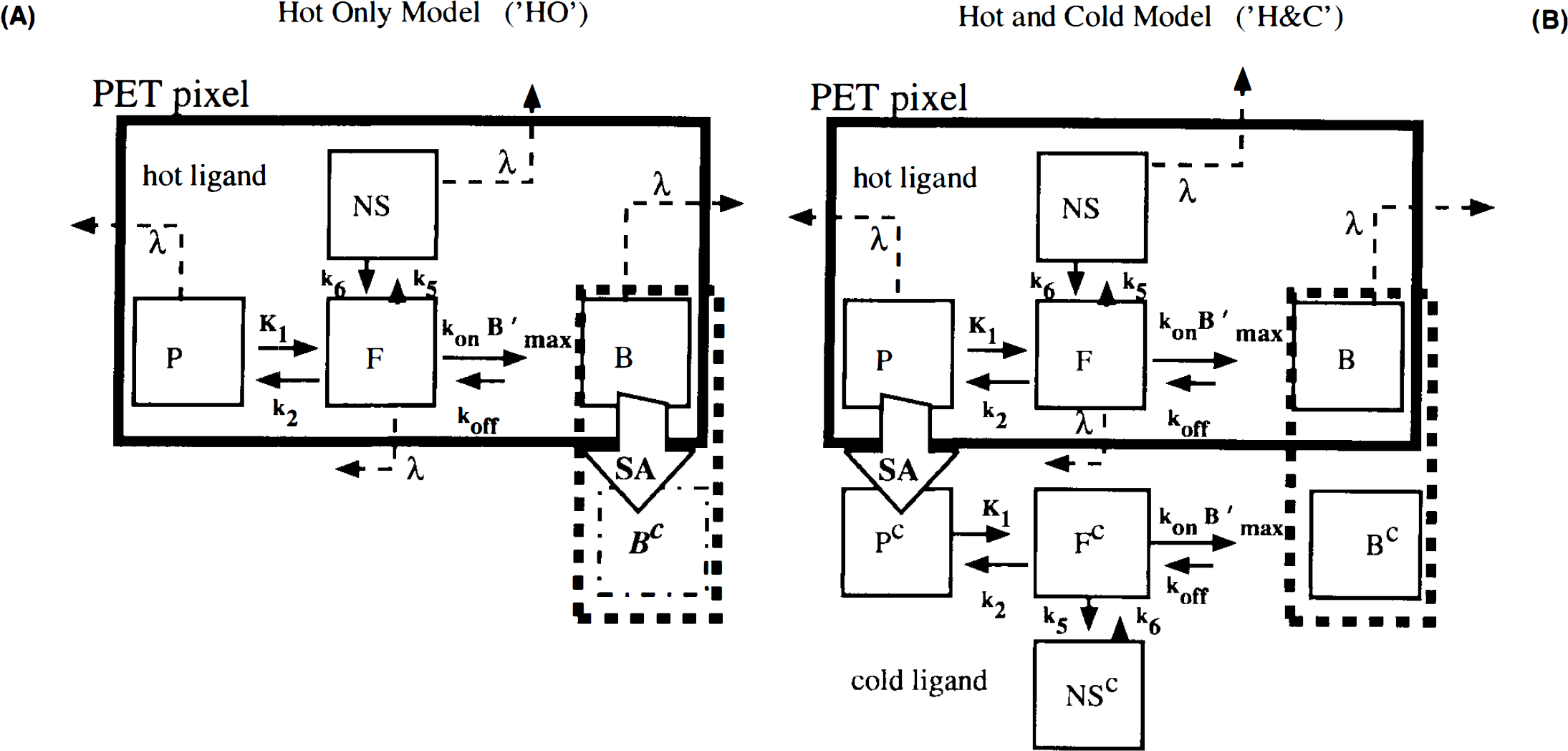
Currently, there are two distinct dynamic modeling approaches to the analysis of multiple-injection PET studies. The first approach (Fig. 1A), chiefly advanced by Bahn and Huang and colleagues (Huang et al., 1989; Bahn et al., 1989) requires simultaneous solution of two or more nonlinear differential equations (i.e., one differential equation per compartment). The second approach (Fig. 1B), advanced by Delforge et al. (1989, 1990, 1991, 1993) is more complex, requiring the solution of twice as many equations. On first glance, the models may seem equivalent since the PET curve in both cases is constructed only from the compartments containing hot ligand. As will be demonstrated below, the models are not the same and should not be used interchangeably for analysis of multiple injection studies. Huang et al. (1989) and Bahn et al. (1989) put forth the first model specifically for simultaneous fitting of data from dual-injection PET studies; this model described only the kinetics of the labeled molecules. A single SA function, which did not distinguish between blood plasma and tissue compartments, was used to calculate the concentration of cold ligand in the bound compartment. This function was modeled as a step, i.e., SA was a constant, SA₁, following the first injection and a constant, SA₂, following the second injection. We have generalized the function, SA(t), to account for the residual effect of all prior injections of hot and cold ligand. We also generalized the nonspecific binding into a distinct compartment and introduced the necessary first order rate constants rather than assuming, as did Mintun et al. (1984) originally, that nonspecific binding would be instantaneous and could be collapsed into the free compartment via a partition coefficient, f₂. We have not retained the dependence of the plasma extraction term, K₁, on the SA of the injectate, since it was found to be minimal (Huang et al., 1989). In 1989, Delforge et al., reported that an initial, high SA injection followed by a completely cold injection would increase the precision of the parameter estimates, perhaps enough to estimate B′_max and K_D separately. A third injection was necessary to isolate a unique solution to the parameter estimation problem. In contrast to the Huang approach, Delforge et al. (1989, 1990) proposed essentially separate models for labeled and unlabeled ligands. The “separate” models are coupled by their bound ligand compartments because the hot and cold ligand molecules compete for the same ligand binding sites, the initial number of which is B′_max.

FIG. 1.

Schematic representations of models described in Eqs. A1–A3 (A) and A4–A9 (B). The hot only (HO) model (A) contains boxes (i.e., compartments) representing the possible states of the labeled ligand, namely, the plasma state (‘P’), free state (‘F’), receptor-bound state (‘B’), or nonspecifically bound state (‘NS’). All of these states of the hot ligand contribute to the PET signal, hence their inclusion in the ‘PET pixel.’ As suggested by the heavy arrow labeled ‘SA,’ the HO model accounts for the effect of cold ligand binding to receptor via the bound concentration of hot ligand, B, and the SA. Losses from each hot compartment, labeled X, represent radioactive decay. The hot and cold (HC) model (B) includes boxes for each of the possible states of both the labeled and unlabeled ligand. The labeled ligand compartments are identical to (A). The states of the cold ligand are the plasma state (‘P^c’), free state (‘F^c’), receptor-bound state (‘B^c’), or nonspecifically bound state (‘NS^c’). The dashed box enclosing the two bound compartments is to emphasize the competition between labeled and unlabeled ligand for a limited number of receptor binding sites. The HC model uses the SA to generate a plasma input function for cold ligand from the measured input function for hot ligand in the plasma. First-order rate constants (labeling each arrow) govern the transition of ligand from one state to another. Free ligand is transformed to bound ligand via its biomolecular association with available receptor sites, hence the shorthand label “k_onB′_max” for the corresponding arrow. Losses from each hot compartment, labeled X, represent radioactive decay; there is no radioactive decay of cold ligand.

Model differences

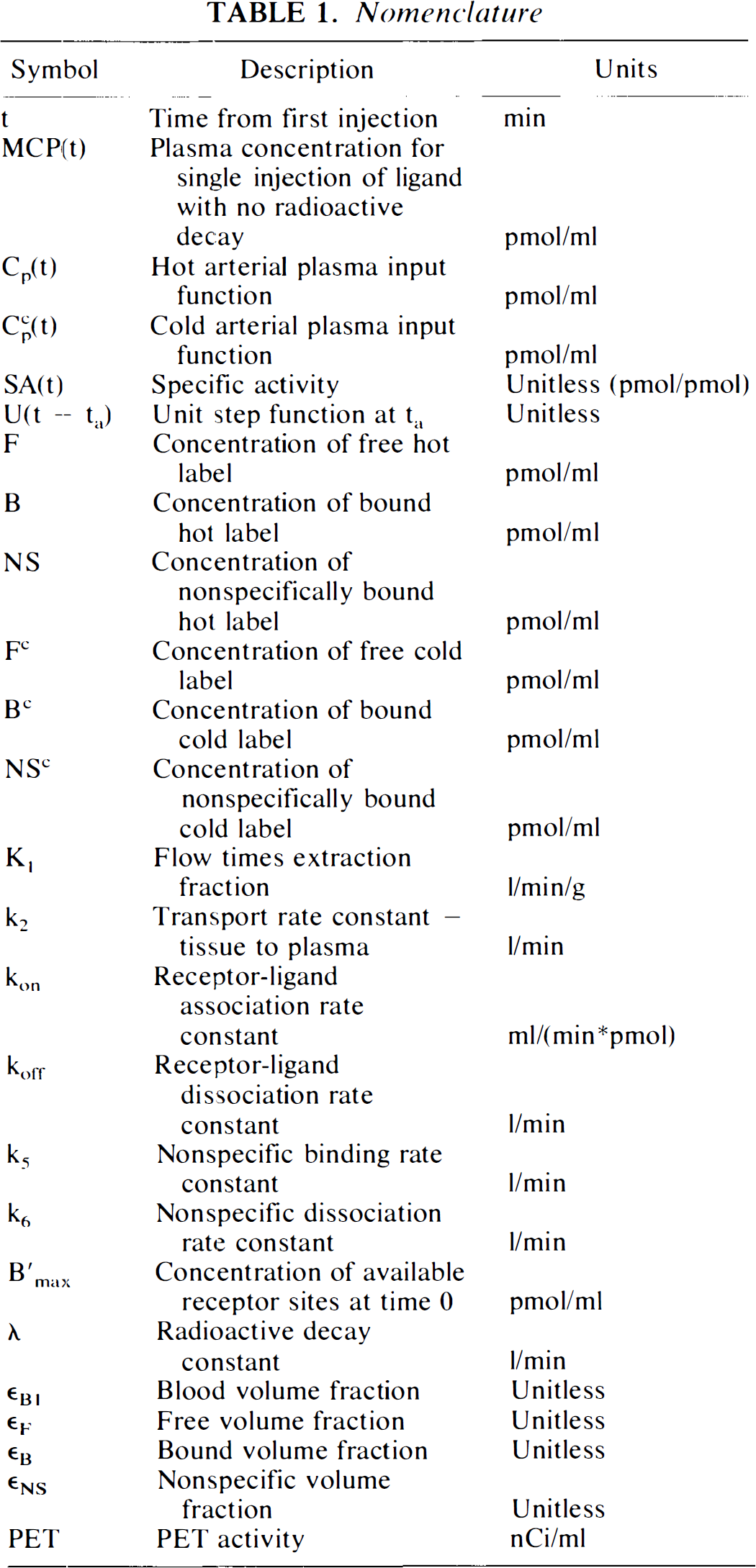
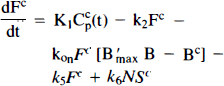
Figures 1A and B schematically depict the two models under consideration. The models allow the ligand to be in four different states: unreacted in plasma, unreacted (free) in tissue, nonspecifically bound, and bound to receptor. Table 1 provides a key to the symbolic notation. Unlike the formulation of Huang et al. (1989), we have included a nonspecific binding compartment that is distinct from the free space. The model equations for this model are

TABLE 1.

Nomenclature

Symbol	Description	Units
t	Time from first injection	min
MCP(t)	Plasma concentration for single injection of ligand with no radioactive decay	pmol/ml
Cp(t)	Hot arterial plasma input function	pmol/ml
Ccp(t)	Cold arterial plasma input function	pmol/ml
SA(t)	Specific activity	Unitless (pmol/pmol)
u(t – ta)	Unit step function at ta	Unitless
F	Concentration of free hot label	pmol/ml
B	Concentration of bound hot label	pmol/ml
NS	Concentration of nonspecifically bound hot label	pmol/ml
Fc	Concentration of free cold label	pmol/ml
Bc	Concentration of bound cold label	pmol/ml
NSC	Concentration of nonspecifically bound cold label	pmol/ml
K1	Flow times extraction fraction	l/min/g
k2	Transport rate constant – tissue to plasma	l/min
kon	Receptor-ligand association rate constant	ml/(min*pmol)
koff	Receptor-ligand dissociation rate constant	l/min
k5	Nonspecific binding rate constant	l/min
k6	Nonspecific dissociation rate constant	l/min
B′max	Concentration of available receptor sites at time 0	pmol/ml
Δ	Radioactive decay constant	l/min
εB1	Blood volume fraction	Unitless
εF	Free volume fraction	Unitless
εB	Bound volume fraction	Unitless
εNS	Nonspecific volume fraction	Unitless
PET	PET activity	nCi/ml

$\begin{array}{lll}\frac{\text{dF}}{\text{dt}}\hfill & =\hfill & {\mathrm{K}}_1{\mathrm{C}}_{\mathrm{p}}(\mathrm{t})-{\mathrm{k}}_2\mathrm{F}-{\mathrm{k}}_{\text{on}}\mathrm{F}\left[{\mathrm{B}}_{max}^{\prime }-\frac{\mathrm{B}}{\text{SA}(\mathrm{t})}\right]\hfill \\ \hfill & \hfill & \hspace{0.17em}+\hspace{0.17em}\hspace{0.17em}{\mathrm{k}}_{\text{off}}\mathrm{B}-{\mathrm{k}}_5\mathrm{F}+{\mathrm{k}}_6\text{NS}-\lambda \mathrm{F}\hfill \end{array}$

(1)

$\frac{\text{dB}}{\text{dt}}={\mathrm{k}}_{\text{on}}\mathrm{F}\left[{\mathrm{B}}_{max}^{\prime }-\frac{\mathrm{B}}{\text{SA}(\mathrm{t})}\right]-{\mathrm{k}}_{\text{off}}\mathrm{B}-\lambda \mathrm{B}$

(2)

$\frac{\text{dNS}}{\text{dt}}={\mathrm{k}}_5\mathrm{F}-{\mathrm{k}}_6\text{NS}-\lambda \text{NS}$

(3)

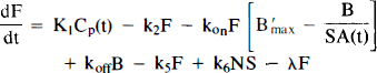
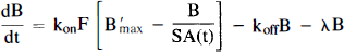
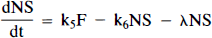
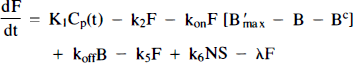
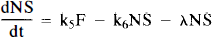
Equations 1–3 are the balance equations for the compartments in Fig. 1A. For convenience, we will refer to this model as the “hot only” (HO) model. The equations for the second model are

$\begin{array}{lll}\frac{\text{dF}}{\text{dt}}\hfill & =\hfill & {\mathrm{K}}_1{\mathrm{C}}_{\mathrm{p}}(\mathrm{t})-{\mathrm{k}}_2\mathrm{F}-{\mathrm{k}}_{\text{on}}{\mathrm{F}[\mathrm{B}}_{\text{max}}^{\prime }-\mathrm{B}-{\mathrm{B}}^{\mathrm{c}}]\hfill \\ \hfill & \hfill & \hspace{0.17em}\hspace{0.17em}+{\mathrm{k}}_{\text{off}}\mathrm{B}-{\mathrm{k}}_5\mathrm{F}+{\mathrm{k}}_6\text{NS}-\lambda \mathrm{F}\hfill \end{array}$

(4)

$\frac{\text{dB}}{\text{dt}}={\mathrm{k}}_{\text{on}}{\mathrm{F}[\mathrm{B}}_{\text{max}}^{\prime }-\mathrm{B}-{\mathrm{B}}^{\mathrm{c}}]-{\mathrm{k}}_{\text{off}}\mathrm{B}-\lambda \mathrm{B}$

(5)

$\frac{\text{dNS}}{\text{dt}}={\mathrm{k}}_5\mathrm{F}-{\mathrm{k}}_6\text{NS}-\lambda \text{NS}$

(6)

$\begin{array}{lll}\frac{{\text{dF}}^{\mathrm{c}}}{\text{dt}}\hfill & =\hfill & \hspace{0.17em}{\mathrm{K}}_1{\mathrm{C}}_{\mathrm{p}}^{\mathrm{c}}(\mathrm{t})-{\mathrm{k}}_2{\mathrm{F}}^{\mathrm{c}}-\hfill \\ \hfill & \hfill & {\mathrm{k}}_{\text{on}}{\mathrm{F}}^{\mathrm{c}}{[\mathrm{B}}_{\text{max}}^{\prime }\mathrm{B}-{\mathrm{B}}^{\mathrm{c}}]-\hfill \\ \hfill & \hfill & {\mathrm{k}}_5{\mathrm{F}}^{\mathrm{c}}+{\mathrm{k}}_6\mathrm{N}{\mathrm{S}}^{\mathrm{c}}\hfill \end{array}$

(7)

$\frac{{\text{dB}}^{\mathrm{c}}}{\text{dt}}={\mathrm{k}}_{\text{on}}{\mathrm{F}}^{\mathrm{c}}[{{\mathrm{B}}^{\prime }}_{\text{max}}-\mathrm{B}-{\mathrm{B}}^{\mathrm{c}}]-{\mathrm{k}}_{\text{off}}{\mathrm{B}}^{\mathrm{c}}$

(8)

$\frac{{\text{dNS}}^{\mathrm{c}}}{\text{dt}}={\mathrm{k}}_5{\mathrm{F}}^{\mathrm{c}}-\hspace{0.17em}{\mathrm{k}}_6{\text{NS}}^{\mathrm{c}}$

(9)

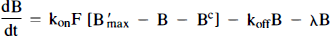
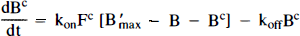
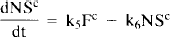
We will refer to the model in Fig. 1B as the “hot and cold” HC model. PET activity in either model is calculated by integrating each hot compartment's concentration over the length of the each scan and summing the values weighted by their respective volume fractions:

$\begin{array}{lll}{\text{PET}}_{\mathrm{i}+1}\hfill & =\hfill & \frac{1}{{\mathrm{t}}_{\mathrm{i}+1}-{\mathrm{t}}_{\mathrm{t}}}{\int }_{\mathrm{t}}^{{\mathrm{t}}_{\mathrm{i}+1}}\hfill \\ \hfill & \hfill & [{\varepsilon }_{\text{Bl}}{\mathrm{C}}_{\text{BL}}+{\varepsilon }_{\mathrm{F}}\mathrm{F}+{\varepsilon }_{\mathrm{B}}\mathrm{B}+{\varepsilon }_{\text{NS}}\text{NS}]\mathrm{d}\mathrm{t}\hfill \end{array}$

(10)

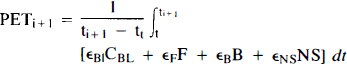
We have assumed for all of our work here that the vascular volume fraction is between 0.03 and 0.05, while the three tissue compartments simultaneously occupy the remaining 95–97% of the total volume.

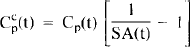
Arrows indicating radioactive loss from each hot compartment with time constant, λ, are included in both parts of Fig. 1 and the corresponding loss terms (containing e^−λt) are included in the model equations where appropriate (see Eqs. 1–6). The dotted compartment, B^c, outside of the PET pixel boundaries in Fig. 1A is not an actual compartment of the HO model but is drawn to indicate that the SA function and the concentration of bound hot ligand are used to calculate the concentration of cold ligand bound to receptor. This relationship is incorporated into Eqs. 1 and 2 via the nonlinear term, k_on-F(t)[B′_max — B(t)/SA (t)], which describes the bimolecular association of free (hot) ligand with available receptor sites. The corresponding balance equations of the HC model (Eqs. 4 and 5) express the available receptor sites explicitly in terms of hot and cold ligand molecules in the bound state, [B′_max — B(t) — B^c(t)].

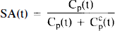
Consider the practical differences between the models. Whereas the HO model formulation requires a single input function, C_p(t), the HC model requires the specification of input functions for both the labeled and unlabeled ligands: concentration of label in plasma, C_p(t), and concentration of cold ligand in plasma, C^c_p(t). Although the hot input function can be measured directly (typically via blood sampling), the cold input function must be inferred as

${\mathrm{C}}_{\mathrm{p}}^{\mathrm{c}}(\mathrm{t})={\mathrm{C}}_{\mathrm{p}}(\mathrm{t})\left[\frac{1}{\text{SA}(\mathrm{t})}-1\right]$

(11)

This relationship between hot and cold inputs in the HC model is indicated in Fig. 1B by the arrow labeled “SA” between the hot and cold plasma compartments. The SA function in Eq. 1 is the same one used in the HO model, but when invoked in the HC model, it refers only to the relationship between hot and cold ligand in the plasma.

Generalized SA function

The analytic expression for specific activity, SA(t), generalized to multiple injections is given below in Eqs. 12–14. It is based on our expectations of the dynamics of ligand molecules injected as a bolus into the blood. In its most general form SA(t) must include the radioactive decay of hot tracer.

$\text{SA}(\mathrm{t})=\frac{{\mathrm{C}}_{\mathrm{p}}(\mathrm{t})}{{\mathrm{C}}_{\mathrm{p}}(\mathrm{t})+{\mathrm{C}}_{\mathrm{p}}^{\mathrm{c}}(\mathrm{t})}$

(12)

For multiple injection studies, the SA. expressed as a unitless ratio of moles of hot to moles of total ligand, is a compound function summed over injections 1 … n.

$\begin{array}{lll}\text{SA}(\mathrm{t})\hfill & =\hfill & \hfill \\ \hfill & \hfill & \frac{\sum _{\mathrm{i}=1}^{\mathrm{n}}\text{MCP}(\mathrm{t}-{\mathrm{t}}_{\mathrm{i}})\mathrm{U}(\mathrm{t}-{\mathrm{t}}_{\mathrm{i}}){\mathrm{e}}^{-\lambda (\mathrm{t}-{\mathrm{t}}_{\mathrm{i}})}}{\sum _{\mathrm{i}=1}^{\mathrm{n}}\text{MCP}(\mathrm{t}-{\mathrm{t}}_{\mathrm{i}})\mathrm{U}(\mathrm{t}-{\mathrm{t}}_{\mathrm{i}}){\mathrm{e}}^{-\lambda (\mathrm{t}-{\mathrm{t}}_{\mathrm{i}})}+}\hfill \\ \hfill & \hfill & \hspace{0.17em}\hspace{0.17em}\hspace{0.17em}\hspace{0.17em}\hspace{0.17em}\hspace{0.17em}\hspace{0.17em}\hspace{0.17em}\hspace{0.17em}\sum _{\mathrm{i}=1}^{\mathrm{n}}\text{MCP}(\mathrm{t}-{\mathrm{t}}_{\mathrm{i}})\mathrm{U}(\mathrm{t}-{\mathrm{t}}_{\mathrm{i}})\hfill \end{array}$

(13)

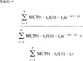
where, for example,

$\text{MCP}(\mathrm{t})=\text{MCP}(0^{+})[{\text{Ae}}^{-\alpha \mathrm{t}}+(1-\mathrm{A}){\mathrm{e}}^{-\beta \mathrm{t}}]$

(14)

Concentration of labeled ligand in the plasma, normally given in units of activity, is converted into molar concentration using the formula for first order radioactive decay: activity = dN/dt = λN, where N is the number of particles and λ is the decay constant of the isotope, U(t — t₁) is the unit step function at the injection time, t₁.

Metabolite-corrected plasma (MCP)(t) is typically a bi-exponential equation that describes the decay-corrected, MCP radioactivity from a single bolus injection. MCP represents only the biological removal of tracer from plasma, distinct from the radioactive decay. The only assumption here is that the biological decay function, MCP, is the same for all injections for labeled and unlabeled ligand. The only exception is the scale of the function, MCP(0⁺), which is the peak concentration of unmetabolized ligand in the plasma. For fast bolus injections (cases 1–3), the peak occurs almost instantly after the start of injection—in such cases, we have fit the plasma radioactivity starting at the peak to a decaying bi-exponential function. Plasma data after each peak were still described by two decaying exponentials. As demonstrated below, the time dependence of SA for multiple injections of different SAs is a complicated function, which typically changes most rapidly immediately following each of the latter injections.

Description of cases examined

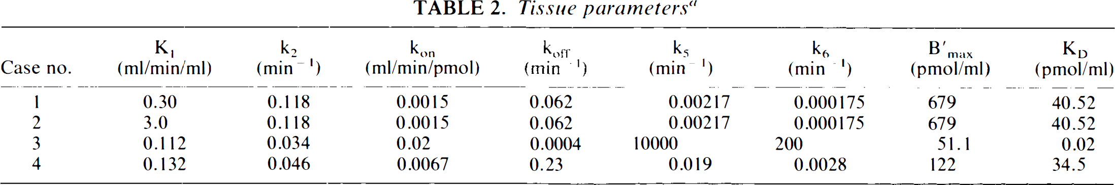
The behavior of the two models were compared for different parameter values and injection protocols, comprising cases 1–4. The cases examined were as follows: case 1, high K_D, large B′_max, complete receptor occupancy (for part of the study); case 2, very high transfer rate constants between plasma, free, and bound compartments; case 3, low K_D, small B′_max, incomplete occupancy; and case 4, high K_D, moderate B′_max, more realistic plasma curve.

Case 1 parameters were based on our preliminary analysis of PET studies with the dopamine transporter ligand, ¹¹C-(CFT), in rhesus monkeys (Macaca mulatto). Case 2 parameters were derived from case 1 with K₁, k₂ increased by one order of magnitude and k_on, k_off increased by two orders of magnitude. Case 3 parameters were taken from subject 3 in the study of Huang et al. (1989). The protocol presented by Huang et al. was extended to three injections in order to examine the response of the system once the second injection had caused partial receptor blockade. Because the University of California at Los Angeles (UCLA) researchers (Bahn et al., 1989; Huang et al., 1989) used an equilibrium fraction, f₂, to partition the free compartment into free and nonspecifically bound ligand as well as a plasma to tissue transport constant, K₁, which was permitted to vary with injection, we had to make certain approximations to their estimated values to conform with our model formulation. We emulated their f₂ value by fixing k₅ and k₆ values at very high numbers in the ratio, k₅/k₆ = 1/f₂, so that our nonspecific compartment would be in instantaneous equilibration with our free compartment, and the fraction, f₂, of the sum of these two compartments would be available for binding to the receptor. Case 4 parameters were based on a subsequent analysis of ¹¹C-CFT data from a multiple injection study of cynomologous monkeys (Morris et al., 1995b); the plasma function used in these simulations represents the actual plasma data acquired. The particular protocols used in Cases 1 and 4 were chosen as the result of a preliminary experimental design optimization study. In short, we chose the times, activities, and SAs of the three injections in order to minimize both the overall variance of the estimates and, specifically, the expected variance in B′_max (Morris et al., 1995a).

Tissue parameters for each case are given in Table 2, plasma parameters are given in Table 3, and injection parameters are given in Table 4. Plasma input curves (for cases 1–3) for multiple injection simulations were constructed by summing bi-exponentials scaled by their respective injected activities, as described in the section on generalized SA function.

TABLE 2.

Tissue parameters^a

Case no.	K1 (ml/min/ml)	k2 (min−1)	kon (ml/min/pmol)	koff (min−1)	k5(min−1)	k6(min−1)	B′max (pmol/ml)	KD(pmol/ml)
1	0.30	0.118	0.0015	0.062	0.00217	0.000175	679	40.52
2	3.0	0.118	0.0015	0.062	0.00217	0.000175	679	40.52
3	0.112	0.034	0.02	0.0004	10000	200	51.1	0.02
4	0.132	0.046	0.0067	0.23	0.019	0.0028	122	34.5

TABLE 3.

Plasma parameters

Case no.	MCP(0+) nCi/ml	A	α (min−1)	β (min−1)
1	32,000	0.901	1.68	0.0625
2	32,000	0.91	1.68	0.0625
3	6,250	0.98	0.80	0.05
	MCP(0.5+) a	A	α	β
4	20,536	0.895	1.36	0.065

a

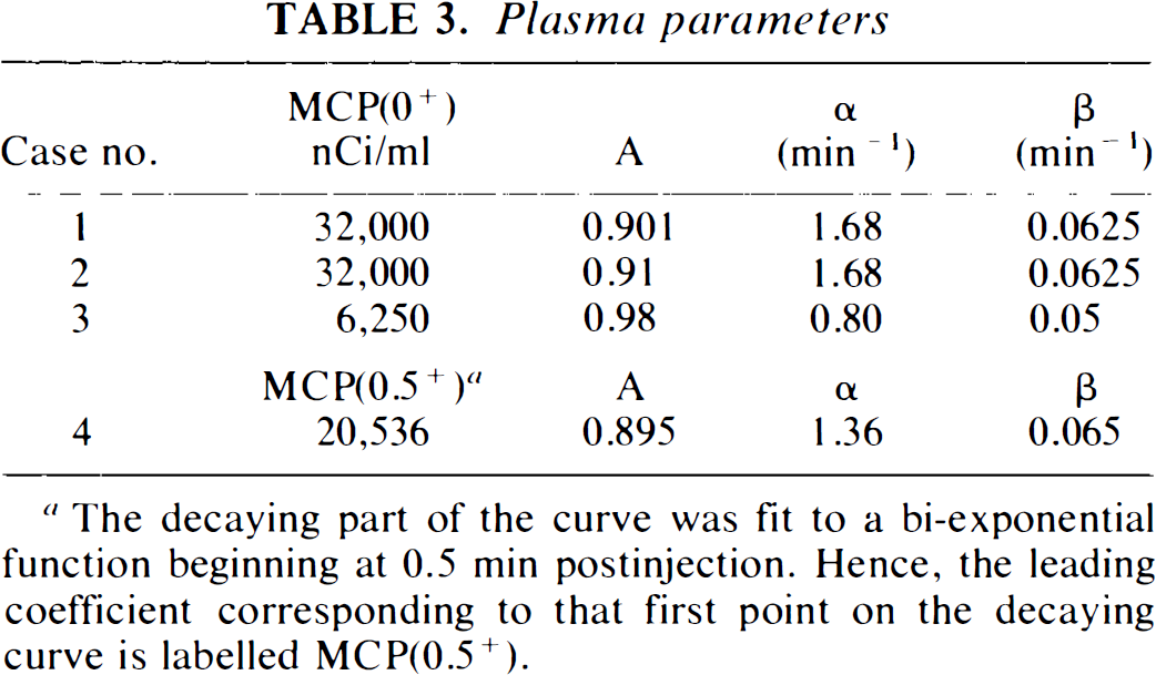
The decaying part of the curve was fit to a bi-exponential function beginning at 0.5 min postinjection. Hence, the leading coefficient corresponding to that first point on the decaying curve is labelled MCP(0.5⁺).

TABLE 4.

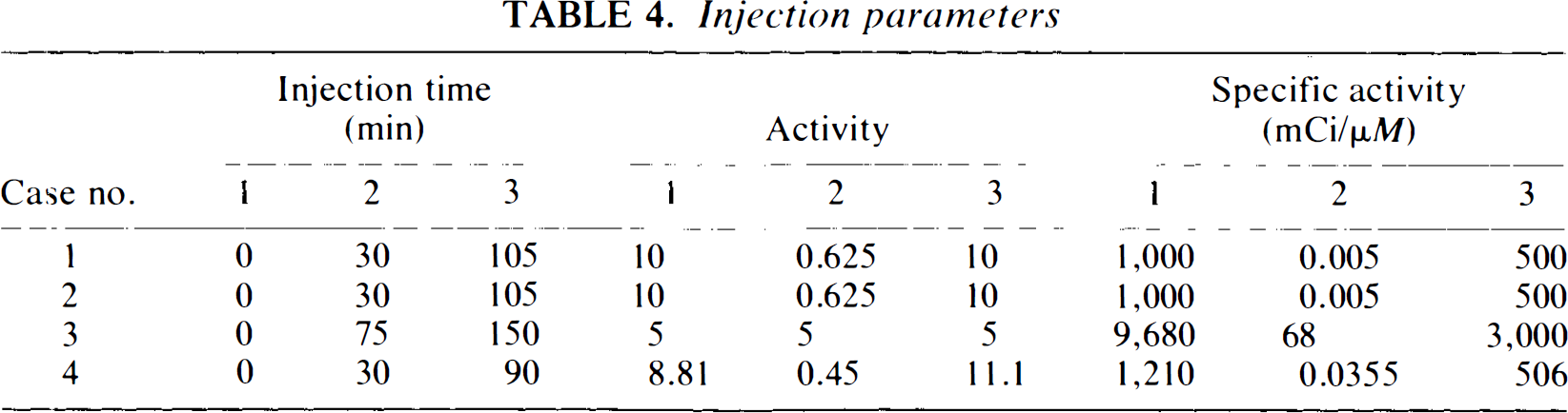
Injection parameters

	Injection time (min)			Activity			Specific activity (mci/μM)
Case no.	1	2	3	1	2	3	1	2	3
1	0	30	105	10	0.625	10	1,000	0.005	500
2	0	30	105	10	0.625	10	1,000	0.005	500
3	0	75	150	5	5	5	9,680	68	3,000
4	0	30	90	8.81	0.45	11.1	1,210	0.0355	506

Generation of test data

We used the HC model to generate test data to be fit by the HO model. Parameters used were the same as given above for the simulations. To generate more realistic test data, we added noise the mean of which was proportional to the square root of the PET signal. Following Mazoyer et al. (1986) and others, we modeled the variance of the measurement error as proportional to the PET signal in the region

${\sigma }^2{\hspace{0.17em}}_{\mathrm{i}}=\mathrm{f}*{\text{PET}}_{\mathrm{i}}/\Delta {\mathrm{t}}_{\mathrm{i}}$

15

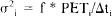
where Δt, is the scan length and f is the proportionality constant that we refer to as the error level. Scan lengths were set uniformly at 1 min throughout the study. For triple injection simulations, specifications for each injection are given in Table 4. Each three-injection simulation was terminated at 170 min, except in case 4, in which the simulation was 120 min long. Scan lengths for case 4 simulations were graduated (30 s for scans within 5 min after the injections and 3 min for later scans).

Numerical simulation and fitting algorithms

All systems of ordinary differential equations were solved numerically with a commercially available software system—IMSL/IDL (Sugar Land, TX, U.S.A.). Weighted nonlinear least squares data fitting was performed using the modified Levenberg-Marquardt routine, NLINLSQ, provided by IMSL/IDL. The weighting matrix supplied to the fitting algorithm consisted of the diagonal elements, σ⁻²_i, which are the inverses of the modeled variances for each residual. When either model was fitted to test data, five parameters (K₁, k₂, k_on, k_off, and B′_max) were allowed to vary, while k₅ and k₆ were fixed at their true values. Estimated values for B′_max using the HC model are given, with error bars that represent one standard deviation as determined from the covariance matrix of the estimates.

RESULTS

Model predictions

One- and two-injection simulations. In the case of a single high SA injection, the number of bound molecules was very small, the available number of receptors ∼B′_max, and the models identical. In fact, the models gave identical PET time activity curves for any single injection simulations. Adding a low SA injection to the experiment (following an initial high SA injection) caused hot ligand to be lost from the bound compartment and a corresponding increase of radioligand in the free compartment. PET curves from the two models for two injections were nearly indistinguishable. Using case 1 parameters (see Methods section), there were only subtle differences between models involving the extent to which the bound label was displaced and the free (and nonspecific) compartment(s) took up the freshly dissociated label (for results of two-injection simulations, see first 105 min of Figs. 2A,B).

FIG. 2.

A: HO model simulation of labeled ligand concentration (pmol/ml) in tissue by compartment for Case 1 parameters. Each curve (p-plasma, b-bound, f-free, n-nonspecific) is multiplied by its respective volume fraction (0.03, 0.97, 0.97, 0.97). The total curve, t, is the sum of the four compartment curves. All curves are generated with an infinite decay constant, λ. B: HC model simulation of labeled ligand concentration by compartment for same (Case 1) parameters as in (A).

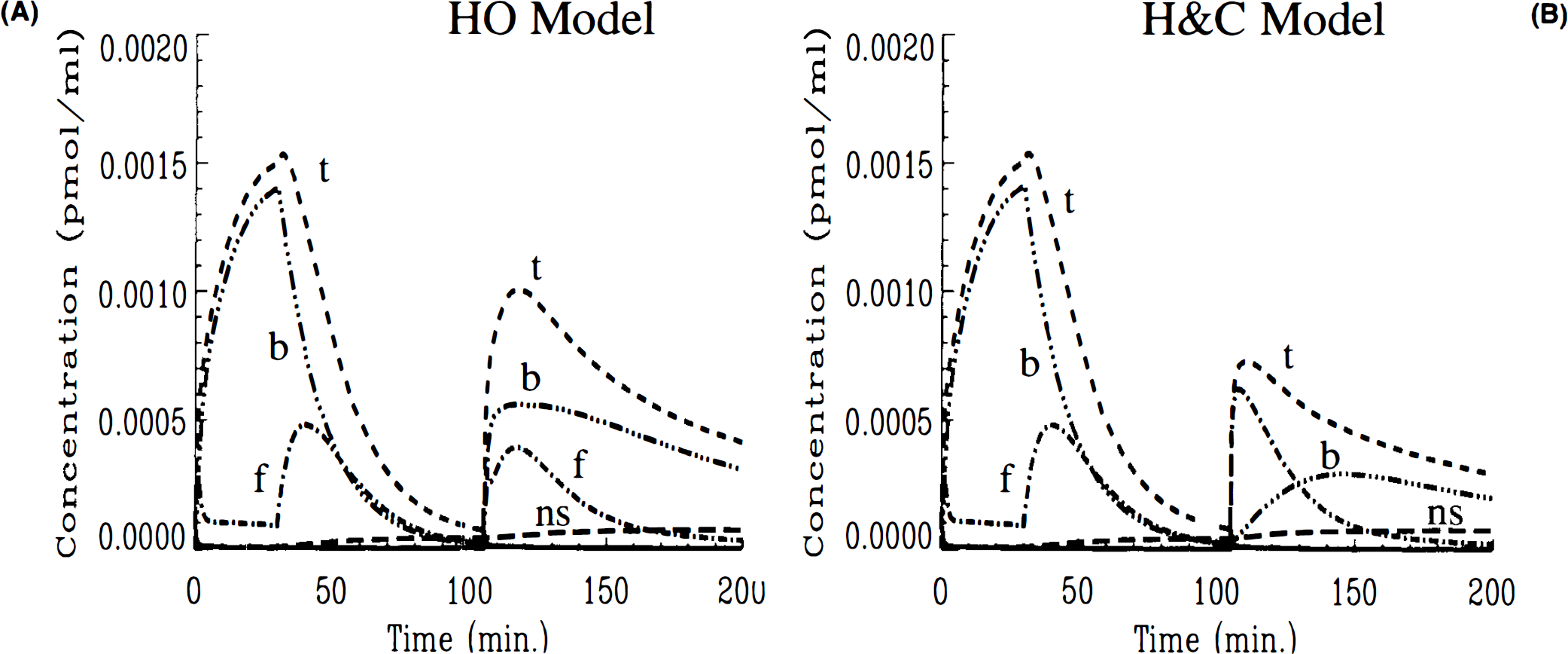
Three-injection simulations of HO and HC models for high K_D, full displacement (case 1)

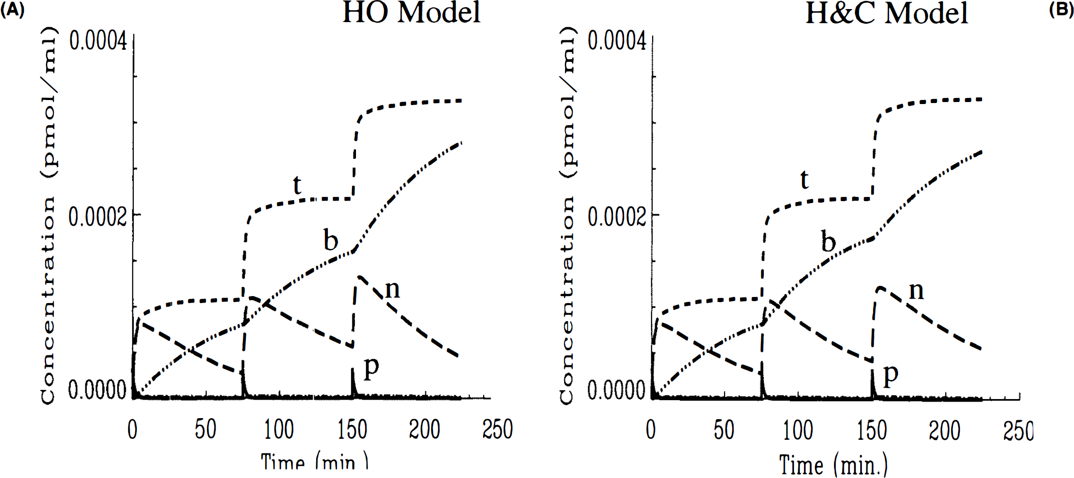
In comparing three-injection simulations, the different behavior of the two models was more readily apparent. Figures 2A,B show the corresponding three-injection simulations of the concentrations of labeled ligand in each compartment of the model as well as the total signal (the total curve corresponds to the integrand in Eq. 10). Both simulations show that the initial high SA injection generates a tissue curve that is largely hot ligand in the bound state. The low SA injection at 30 min causes loss of the hot ligand from the bound compartment until nearly all of it has been displaced. However, after the (high SA) injection at 105 min, the HO model (Fig. 2A) predicts a much more rapid increase in the amount of bound hot ligand than does the HC model (Fig. 2B). Conversely, free hot ligand does not reach as high a concentration according to the HO model as with the HC model. The overall difference is that the total curve in Fig. 2A peaks for the second time at 120 min at ∼0.001 pmol/ml, while the total labeled ligand in Fig. 2B peaks at 110 min at just 0.0007 pmol/ml. Furthermore, the bound curve in the HO model nearly reaches its peak value instantly after the third injection, whereas the same curve in the HC model increases gradually. According to the HC model, the bound compartment does not peak until nearly 140 min, i.e., 35 min after the last injection.

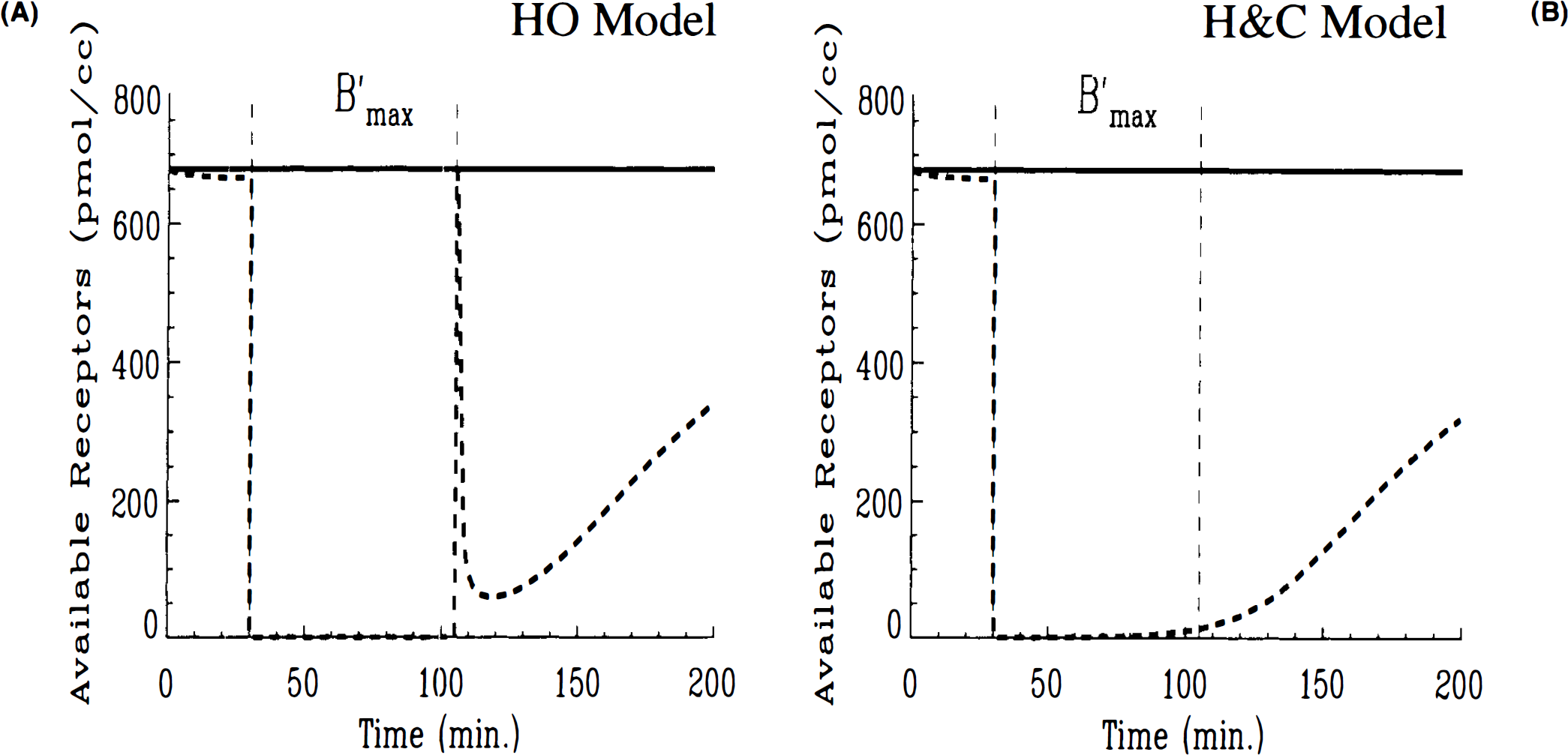
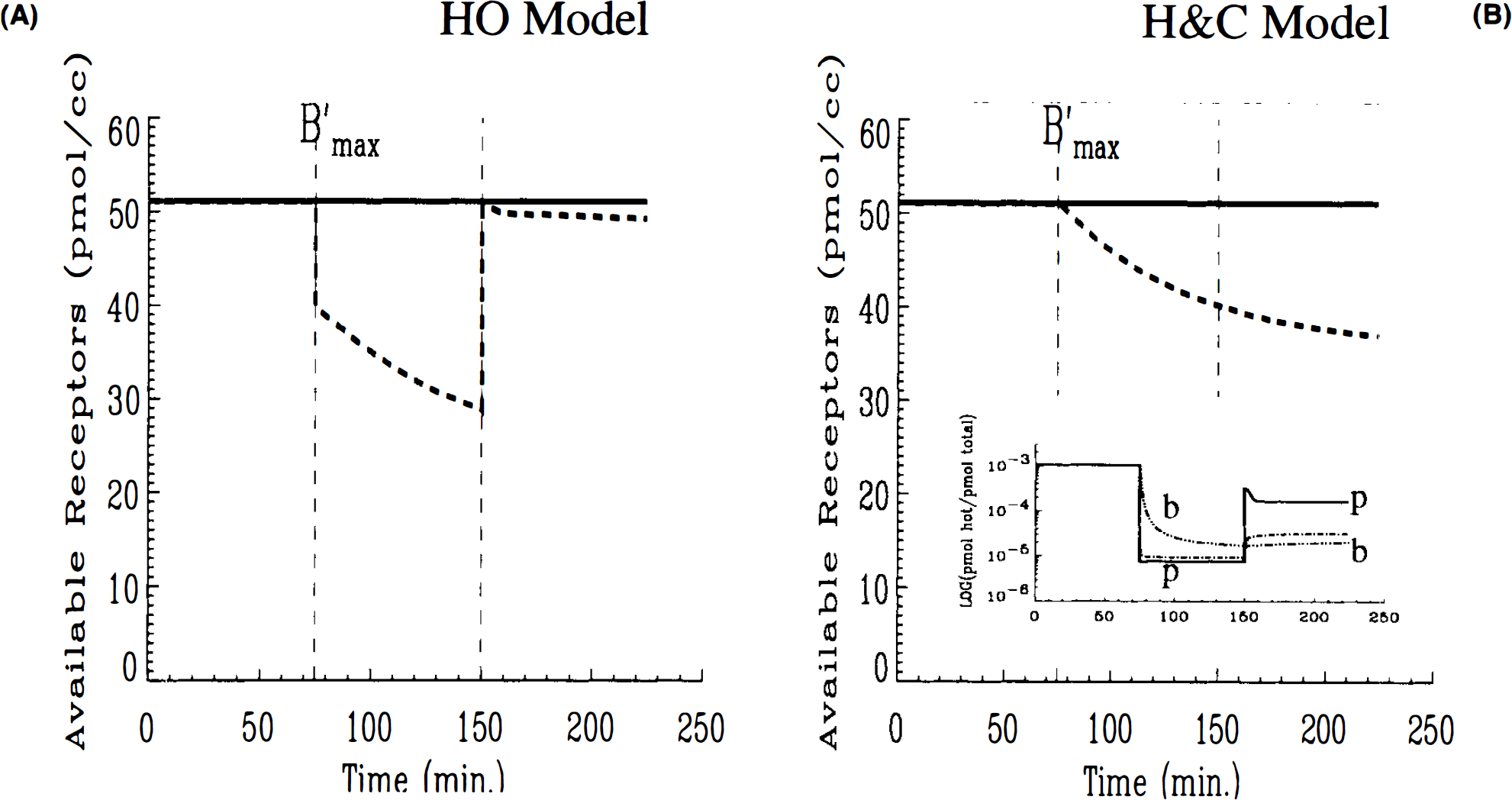
The differences between HO and HC can be understood further by plotting the available number of receptors (in pmol/ml) predicted by each model (Figs. 3A,B). In both cases, the receptor availability is barely affected by the first high SA injection. Following the low SA injection, the introduction of a blocking dose of cold ligand causes the availability of receptor sites to drop precipitously to zero in both cases. While the receptors remain completely blocked in the HO simulation right up until the third injection, there is a slight gradual rise in the number of available receptors in the HC simulation. This gradual rise continues after the injection at 105 min. In fact, the gradual increase in the number of open receptor sites continues (Fig. 3B) for the HC model independently of the third injection. The HO model (Fig. 3A) predicts no freeing up of receptor sites prior to injection three and a transient spike in available receptors to near maximum, B′_max, immediately following the injection. Once the spike in receptor availability dissipates, the model predicts a gradual rise in open sites paralleling the other model. The possibility that numerical artifacts, e.g., round-off error, could have caused the transients in the receptor availability plot was investigated and found not to be a source of error. As we discuss in detail below, the difference in behavior of these two models relates to their respective applications of the SA function.

Fig. 3B.

A: HO model prediction of availability of receptor sites (pmol/ml) in tissue for Case 1 parameters (dashed curve) corresponding to simulated multiple injection experiment shown in Figure 2A. Horizontal (solid) line indicates total number of available sites, B′_max, prior to injection of ligand. Thin vertical dashed lines indicate time of injections. B: HC model prediction of availability of receptor sites for same (Case 1) parameters and experimental protocol.

Simulated SA curves

Recall from the model differences section, above, that the number of available receptors, shown in Fig. 3A is calculated as

${\mathrm{B}}_{\text{available}}(\mathrm{t})={\mathrm{B}}_{max}^{\prime }-\mathrm{B}(\mathrm{t})/\text{SA}(\mathrm{t})$

(16)

whereas in Fig. 3B, the same quantity is calculated as,

${\mathrm{B}}_{\text{available}}(\mathrm{t})={\mathrm{B}}_{max}^{\prime }-\mathrm{B}(\mathrm{t})-{\mathrm{B}}^{\mathrm{c}}(\mathrm{t}).$

(17)

The SA function in Eq. 6 explicitly regulates the relationship between HC ligand in the bound state. To solve the HO model, one must supply an analytic expression for this function. The function we used is the generalized SA function developed above. In the HC model, the SA relationship between HC bound ligand, SA_B(t) = B(t)/[B(t) + B^c(t)], can be calculated directly as a consequence of solving all the state equations for hot and cold ligand in each compartment. An analytical SA function must be supplied to the HC model in the input function (Eq. 11). To see how SA_B(t) differs from SA(t), SA in the plasma, we plot the log of SA by compartment (Fig. 4) based on the solution of the HC model. The curves do not include radioactive decay. The curve labeled ‘p’ is the generalized SA function that appears in the nonlinear term of the HO model and is described in analytical form, above (see Eqs. 12–14). Curves labeled ‘f’ and ‘b’ are the SAs in the free and bound compartments, respectively, calculated by the HC model.

FIG. 4.

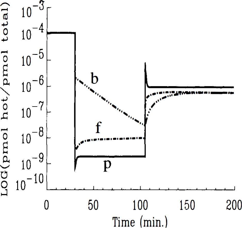
Log of SA by compartment versus time. Simulated via HC model using Case 1 parameters. Curves are generated with an infinite decay constant, λ. SA in all compartments are identical for period following first injection.

One unexpected, but characteristic, result of plasma SA simulations was the over- and undershoots in the curve just after injections. That is, for systems without radioactive decay, a compound plasma curve whose decaying portion we describe as a sum of bi-exponentials (Eq. 14) yields a SA function that is more complicated than a series of constant levels between injections. The sizes of the over- and undershoots are related to the relative sizes of the decay constants, α and β, in the plasma equation.

Three-injection simulations of HO and HC models for very high rate constants (case 2)

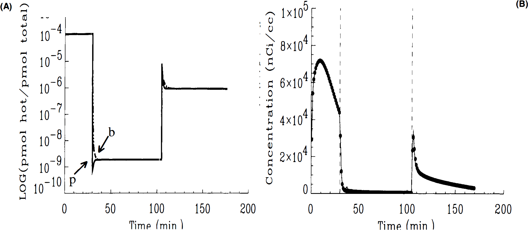
Based on our observation that the discrepancy between SA in the plasma and bound compartments correlates with the divergent behavior of the two models, we sought to identify regions of parameter-space for which the two models were indistinguishable for multiple injections. We hypothesized that if rate constants in the system are high enough, the receptor compartment should equilibrate rapidly with the plasma compartment, thus equalizing their respective SAs. Through a series of simulations, we found that an order of magnitude increase in the values of K₁ and k₂, and an increase of two orders in k_on and k_off were sufficient to cause the SAs in each compartment to very nearly converge to a single curve (see Fig. 5A). The bound SA, SA_B(t), simulated via the HC model, is coincident with the generalized SA function everywhere except in the transients immediately following the latter injections. In turn, the PET activity curves predicted by the two competing models are nearly identical for case 2 parameters (Fig. 5B), except, perhaps, for a mild discrepancy in the peak following the last injection. In Fig. 5B, the HO model is displayed as a solid curve while the HC model is displayed as individual points. It should be noted that the rate constants required to make the models behave identically are quite high and are unlikely to correspond to any receptor ligands.

FIG. 5.

A: Log of SA by compartment versus time for Case 2 parameters simulated via HC model. SA in all compartments are virtually superimposable except immediately following the injections. B: Simulated PET activity curves for HO model (solid line) and HC model (filled circles) for same Case 2 parameters. Curves are identical except perhaps at the peak (105 min) corresponding to the third injection. Curves are generated with an infinite decay constant, λ. Vertical dashed lines indicate time of injections.

Three-injection simulations of HO and HC models for small K_D, partial displacement (case 3)

We looked next at a set of published parameters and injection specifications for the irreversible D₂ antagonist spiperone. One might postulate that if high rate constants narrowed the differences between plasma and bound SA (and, thus, between the predictions of the HO and HC models), then low rate constants might guarantee inequality of the models. We chose to make an additional comparison of models using published parameter values sufficiently different from those in cases 1 and 2 and with a clinically feasible experimental protocol. The case 3 parameters, used in Figs. 6 and 7 are derived from Huang et al. (1989), who estimated model parameters for the irreversible ligand, [¹⁸F]fluoroethyl-spiperone. As listed in the Methods section, the first injection in case 3 is at high SA, while the second is at an intermediate level, which causes incomplete occupancy of the D₂ receptors. The portion of the case 3 simulation for the HO model (Fig. 6A) corresponding to the first two injections appears quite similar to the curves published in Huang et al., 1989 for their two-injection experiments. To examine the behavior of both models after introduction of a large dose of cold, we added a third relatively high SA (3,000 mCi/μmole) injection and spaced the injections every 75 min.

FIG. 6.

A: HO model simulation of labeled ligand concentration (pmol/ml) in tissue by compartment for Case 3 parameters. Each curve (p-plasma, b-bound, n-nonspecific and free) is multiplied by its respective volume fraction (0.05, 0.95, 0.95). The total curve, t, is the sum of the four compartment curves. All curves are generated with an infinite decay constant, λ. The free and nonspecifically bound ligand in these simulations are combined and are both labeled (n) for nonspecific. The partition parameter f₂ = 0.02 used in Huang et al. (1989) means that most (98%) of the free plus nonspecific ligand at any time is unavailable for binding to the receptor. B: HC model simulation of labeled ligand concentration by compartment for same (Case 3) parameters as in (A).

FIG. 7.

A: HO model prediction of availability of receptor sites (pmol/ml) in tissue for Case 3 parameters (dashed curve) corresponding to simulated multiple injection experiment shown in Figure 6A. Horizontal (solid) line indicates total number of available sites, B′_max, prior to injection of ligand. B: HC model prediction of availability of receptor sites for same (Case 3) parameters and experimental protocol. Vertical dashed lines indicate time of injections. Inset shows corresponding HC simulation of specific activity plots for each compartment: bound (b), free and plasma (p).

Unexpectedly, predicted outputs for the two models for Case 3 parameters (Figs. 6A and B) were nearly identical throughout the course of the simulated experiment. However, when we examined each model's prediction of available number of receptor sites, the difference between the two models emerged. Receptor availability, as predicted by the HO and HC models, is displayed in Fig. 7A and B, respectively. There was agreement between the models that the moderately low SA injection (68 mCi/(μmole) at 75 min was insufficient to cause >50% occupancy of available receptor sites at any time during the experiment. Nevertheless, there was a significant difference in the time course of receptor availability predicted by the two models. This discrepancy, which is reminiscent of that shown in Fig. 3, centers on the apparent, high sensitivity of the HO model prediction to abrupt changes in injected SA (notice the abrupt drop and equally sharp rise in receptor availability following the second and third injections). Contrast the behavior of the curve in Fig. 7A to the apparent in-sensitivity to change in injected SA of the curve in Fig. 7B. Notice, in particular, the lack of any change in slope following the introduction of a final high SA ligand at 150 min. The HC model predicts a steady but slowing reduction in the number of open sites pursuant to a moderately low SA injection at 75 min and no discernible rise in the number of available receptor sites with the introduction of a final high SA injection (i.e., small mass of ligand molecules) at 150 min. To be certain that the calculations for B_available shown in Fig. 7 were not artifactual, we examined each of the individual terms that comprise B_available for each model as given in Eqs. 16 and 17. The plots of each component of available (data not shown) clearly indicated that the abrupt—and seemingly nonphysiological—changes in the predicted curves, in the case of the HO model, result from abrupt changes in the (plasma) SA(t) term. On the other hand, B_available predicted by the HC model changes gradually because each of its contributing components, B′_max, B, and B^c are either constant or change gradually. The plot of SA by compartments generated by the HC model is inset in Figure 7B. The inset plot shows that for the particular parameter set and protocol of case 3, SAs in the plasma and bound compartments do not converge following the third injection. Similarly, receptor availability plots do not converge.

Parameter estimation

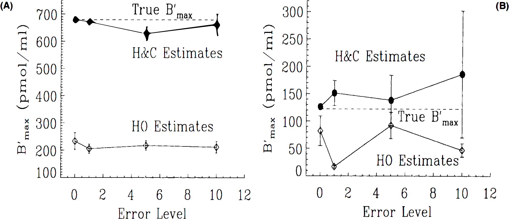
Finally, we contrasted the respective abilities of each model to recover the true parameter values from test data. Figure 8A portrays the estimated values for B′_max based on fitting both models to test data generated with the HC model and case 1 settings. The true value of B′_max is indicated on the graph. As the error level in the simulated data is decreased, the estimated value of B′_max converges to the true value, and the precision of the estimate improves. Estimates based on the HO model are consistently very low and do not improve as the data become less noisy. B′_max values at every error level were underestimated by ∼60%. Similarly, for case 4 parameters, the HC model is able to recover a value approaching the true B′_max as the noise in the data decreases. As shown in Fig. 8B, the HO model is unable to recover the true B′_max value regardless of error level. The error in B′_max with each fit of the HO model is ∼30% of the true value. Based on these two studies, the HO model appears to yield inaccurate estimates of receptor density. Although each datum point represents a single fit to test data, the repeated underestimate of B′_max by the HO model suggests that it yields biased estimates relative to the HC model.

FIG. 8.

A: Estimates of B′_max using both HO and HC models for varying amounts of noise added to 3-injection test data (generated with Case 1 parameters). The test data at each error level was generated with the HC model. True B′_max value in each test data set is 679 pmol/ml—indicated by the dashed line. Estimates using HO model to fit data are indicated by open diamonds. Estimates using HC model are indicated by filled elipses. Points represent single fits to test data sets. Error bars are predictions based on the diagonal elements of the covariance matrix of the estimates and the known error level of the data. B: Estimates of B′_max for varying amounts of noise added to test data sets are based on Case 4 parameters. True value of B′_max = 122 pmol/ml. In both Figs. A and B, the variance of the test data varies linearly with ‘Error Level.’

DISCUSSION

The two different compartmental models that are frequently employed for predicting PET activity curves from multiple injections of labeled neuroreceptor ligand were compared and found not to be equivalent. Since the receptor sites are known to be saturable, each model must account for the presence of cold ligand, which, although it doesn't contribute to the PET signal, does compete with the hot ligand for the limited receptor sites. Differences between the models can be traced to their respective treatments of the effect of cold ligand in the system, specifically, cold ligand in the bound compartment. This difference becomes of paramount importance when the injection of a large dose of cold ligand causes a large fraction—but not necessarily all—of the available receptor sites to be occupied. To account for action of cold ligand, either model must make use of the specific activity (SA) of the ligand since the cold cannot be measured independently. Since both cold and hot ligand concentrations are included explicitly in the HC model, it can be thought of as solving continuously for SA in each compartment. Alternatively, the HO model must use an analytical expression for SA, which, in the best of circumstances, applies only to the plasma compartment and is an approximation to SA in the bound compartment. The generalized SA was introduced to account for effects of all previous injections. Although some of our simulations are based on simple (bi-exponential) representations of the plasma activity, our results hold for more realistic plasma curves as well.

Variations of the HO model seem to predominate in the literature over the HC approach. One question for users of the HO model is: when can the SA of the plasma compartment serve as an adequate approximation of the SA of the bound compartment? Consider that the SA of the ligand is actually measured only prior to injection into the plasma compartment. The SA, which in our usage is the ratio of hot to total ligand, is not changed by dilution of the injectate into the plasma. Nor is it changed by traversing the barriers between tissue compartments as long as the hot and cold ligands have identical access to each compartment. Once second and third injections of ligand are introduced at varying SAs, SA in the tissue compartments becomes more difficult to predict. (Consider the extreme case of a completely irreversible ligand: if enough material were injected in the first injection to occupy all the receptor sites, the SA of the bound compartment would remain at the initial SA indefinitely.) Slow rate constants and/or limited receptor sites slow the ability of the extravascular compartments to assume the SA of the plasma instantaneously. Plasma SA is then no longer a faithful approximation of SA in the bound compartment. We confirmed this picture by showing that for fast transport parameters, SA curves for all compartments are nearly superimposable. Nevertheless, we readily admit that the parameters used for case 2 are not likely to be encountered by researchers imaging practical receptor ligands. Mathematically, SA must be uniform across all compartments for a single injection. If multiple injection studies could be treated as a series of single injections, then it might be argued that SA could be modeled as a series of constant values, and the equivalence of the two models would be preserved. However, once multiple injections are introduced into the plasma compartment, persistence in the plasma of cold ligand from previous injections contributes to plasma SA thereafter. The SA in the plasma becomes a nonintuitive time-varying function that is usually more complicated than a series of steps and, more importantly, no longer bears much resemblance to the SA at the point of interest—the bound compartment.

A three-injection study with high K_D and large cold dose in injection no. 2 (case 1) was examined. For these parameter values, which derived from preliminary experimental work with a dopamine re-uptake inhibitor, the differences between HO and HC models were quite apparent in the PET curves for multiple injection simulations. Furthermore, once we plotted the receptor availability as predicted by each model, it became increasingly clear that the HO model predicted a nonphysiological discontinuity in receptor availability following the third injection. The sharp rise in predicted receptor availability is a direct result of the abrupt change specified in the analytical SA function. These findings were corroborated by our examination of case 3 parameters (low K_D, partial displacement with low SA injection). The PET curves for the two models looked the same but on examination of predicted receptor availability, model differences emerged. As in case 1, the HC model predicted a gradually decreasing receptor availability after the low SA second injection that was unaffected by a later injection of a small amount of high SA ligand. In contrast, the HO model predicted an abrupt drop in receptor availability immediately after the second injection and an equally abrupt rise after the third. We believe that the ability of the model to correctly predict receptor availability is not an insignificant issue. It may be crucial when using PET to measure the effectiveness of neuropsychiatric drug treatment on schizophrenics, for example, so that we be able to determine how many dopamine D₂ sites remain available after haldol administration or how many serotonin 5-(HT) sites remain free after treatment with an atypical neuroleptic.

As the more general of the two, we considered the HC model to be our reference and sought to determine when, if ever, the simpler HO model would be equivalent to it. Our real interest, though, was in the ability of these models to predict ligand behavior in multiple injection studies because there is evidence that a minimum of three injections is needed for identification of all (seven) model parameters (Delforge et al., 1990). Interestingly, in the Huang et al. (1989) study of D₂ receptors with [¹⁸F]-fluoroethyl-spiperone, the authors were able to reproducibly estimate six parameters with an HO-type model and dual-injection data by constraining the K_D value. Is it possible that, despite the reproducibility of their results, the HO model was a source of bias in their estimates?

The question of biased estimates was addressed by attempting to recover B′_max values from test data of different error levels (test data were produced with the HC model). In each of two separate cases examined, fits with the HC model were able, not surprisingly, to consistently recover B′_max values. The smaller the error in the data, the more precise the parameter estimates. Under no circumstances, however, were we able to recover B′_max by fitting the HO model to the test data. In all cases, estimates were significantly different and consistently lower.

The “correctness” of one or the other model could not be determined unequivocally, but the equivalence of the models was tested and found to be unequal. The only indications we have that the HO model is incorrect are that (a) it is intuitively unsatisfying to use the analytical SA function in the bound compartment when we now know it is incorrect and, (b) more tangibly, the HO formulation leads to predictions of receptor availability that seem unrealizable. In fact, neither model might be correct for many popular receptor ligands. For example, if one scrutinizes the fitted curves in Delforge et al. (1990, 1991), there is a hint of the poor residual behavior that we observed when fitting HO model to HC-generated data (data not shown). Yet, those authors have taken the HC approach (in fact, they originated the approach). Perhaps this phenomenon is the result of more than one receptor site for the ligands in question. On the other hand, Votaw et al. (1993) describe the inability of a generalized HO model to properly adequately describe their PET data immediately following a low SA second injection. Their model does include separate compartments for HC ligand, but they have retained explicit inclusion of the SA and, thus, their model may be subject to the limitations of an HO-type approach.

The following caveat is offered to investigators interested in using kinetic models to estimate parameters. Even when the two models seem identical vis-a-vis the forward problem, i.e., they predict similar PET curves (as in case 3), they will not necessarily behave identically in the more important inverse problem, namely parameter estimation. Most estimation methods rely explicitly or implicitly on the model equations and the gradient information. Components of the gradient are the derivatives of the compartmental concentrations with respect to the parameters, and they determine the shape of the objective function to be minimized. Components of the gradient are the derivatives of Eqs. 1–3 or 4–9, respectively, integrated over time. Inspection of these equations reveals that the receptor availability term (B′_max — total bound) figures prominently in many of them. If this term is calculated incorrectly, the direction of each step in the estimation procedure will be affected adversely, possibly forcing the search algorithm into an undesired local minimum of the objective function in parameter space. Thus, even though two models may predict similar output curves for a given set of parameters, owing to a multiplicity of nearly equivalent local minima, they may not yield the same parameter estimates to a given set of PET data.

CONCLUSION

In this study, we have compared the behavior of the two models most widely cited in the literature for describing the kinetics of a neuroreceptor ligand, as measured by dynamic PET studies. The HO model, although used widely in various forms, is not equivalent to the HC model, which is less well known. The differences are not always apparent in the PET curves predicted by each model. In fact, the models are identical for single injection studies and for multiple injection studies for rapidly equilibrating tracers. However, proper analysis of multiple injection protocols, including at least one large dose of cold ligand, requires an accurate representation of the available number of receptor sites over time. Without including explicit compartments for the cold ligand in the model, receptor availability must be calculated by applying the plasma SA in the bound compartment. As we have demonstrated, SA, which is only reasonably well known for the plasma compartment, can actually be significantly different in the bound compartment. Improper use of the SA function will lead to unrealistic predictions of receptor availability and to biased estimates of model parameters (e.g., B′_max). There is mounting evidence that multiple injection studies are necessary to characterize the kinetic parameters associated with many neuroreceptor ligands. As these complex studies become more commonplace for studying the behavior of particular ligands/drugs and for measuring the number of receptor sites left unblocked by a particular drug therapy, we believe that use of the HC model will become essential for the proper quantitative analysis of PET data.