
Abstract
Determining the appropriate sample size is a crucial component of positron emission tomography (PET) studies. Power calculations, the traditional method for determining sample size, were developed for hypothesis-testing approaches to data analysis. This method for determining sample size is challenged by the complexities of PET data analysis: use of exploratory analysis strategies, search for multiple correlated nodes on interlinked networks, and analysis of large numbers of pixels that may have correlated values due to both anatomical and functional dependence. We examine the effects of variable sample size in a study of human memory, comparing large (n = 33), medium (n = 16,17), small (n = 11, 11, 11), and very small (n = 6, 6, 7, 7, 7) samples. Results from the large sample are assumed to be the “gold standard.” The primary criterion for assessing sample size is replicability. This is evaluated using a hierarchically ordered group of parameters: pattern of peaks, location of peaks, number of peaks, size (volume) of peaks, and intensity of the associated t (or z) statistic. As sample size decreases, false negatives begin to appear, with some loss of pattern and peak detection; there is no corresponding increase in false positives. The results suggest that good replicability occurs with a sample size of 10–20 subjects in studies of human cognition that use paired subtraction comparisons of single experimental/baseline conditions with blood flow differences ranging from 4 to 13%.
Studies of human cognitive functions using [15O]H2O have been conducted for over a decade. Although statistical techniques for analyzing positron emission tomography (PET) data have become increasingly sophisticated (Mintun et al., 1989; Fox, 1991; Worsley et al., 1992; Friston et al., 1993–1995), several statistical issues have not as yet been addressed. One of the most important of these is the appropriate sample size for producing robust and replicable results. Since PET studies are costly to perform and require radiation exposure to human subjects, identifying the smallest possible sample to answer a question or test a hypothesis as conclusively as possible is an important priority. Yet very few empirical data have been assembled to address this issue.
Sample sizes in most water studies tend to be relatively small. A review of 75 recent studies conducted using the [15O]H2O method indicates that sample size ranges from 4 to 34, and the median is 9. The majority of studies to date have used an exploratory data analysis strategy, sometimes referred to as the “function-of-interest” approach (Arndt et al., 1995); this strategy uses techniques derived from inferential statistics, such as analysis of variance, that were developed for testing a limited number of hypothesis. The application of these techniques to the 150,000-pixel data sets analyzed in the typical PET experiment creates challenges in interpretation, because of the large number of statistical tests performed. Another approach, involving an initial function-of-interest approach followed by a hypothesis-testing analysis based on regions of interest in a second independent sample, offers a second alternative, although one that doubles sample size (Buckner et al., 1995; Drevets et al., 1995).
Conventionally, sample size for scientific experiments is selected on the basis of a power analysis (Cohen, 1988). Our review of 75 recent PET studies indicated that 44 had a power of ≤0.5, suggesting that they may be underpowered. However, power analysis may not be the most appropriate approach for identifying adequate sample size for PET data analysis. Power calculations assume that the magnitude of t and its associated significance level are the primary concerns. PET data present unique problems, because of the facts that the data points tend to be correlated with one another, the correlations between data points are in themselves an object of interest since they may help in identifying cognitive networks, and the number of adjacent pixels activated may be more important than the size of the t statistic. Conventional power calculations were not designed to take into account the simultaneous assessment of multiple interrelated measurements of variable importance.
We report herein on a study designed to explore the question of sample size in PET experiments using empirical data. The primary purpose of this study was to examine issues inherent in the determination of sample size for PET experiments and to identify some general principles involved in establishing the appropriate sample size for conducting investigations of human cognition using the [15O]H2O method with PET.
METHODS
The basic design of this study involved beginning with analyses conducted with a large sample (n = 33), collected in an experiment that was designed to explore mechanisms of human memory (Andreasen et al., 1995). The results of these analyses were assumed to be the “gold standard.” This sample was then subdivided into three progressively smaller groupings (n = 16 or 17 = “medium,” n = 11, 11, 11 = “small,” and n = 6,6,7,7,7 = “very small”). These smaller sample sizes are similar to those usually reported in most PET studies conducted to date.
In addition to examining the effect of varying sample size, we also examined the effect of variation in the intensity of the activation. As we and others have shown, familiarity with a task may make performance more automatic and efficient, thereby reducing the size of the brain region activated and the size of the associated t statistic (Raichle et al., 1994; Andreasen et al., 1995). Novel tasks may produce larger areas of activation with higher t values. Thus, we chose to compare two memory tasks that were similar in many respects, but that differed in the amount of practice provided to the subjects and consequently in the intensity and size of activation. The design of this study permits us to compare the effects of sample size on the measurement of blood flow during two complex cognitive tasks with larger or smaller activation effects using the same individuals.
Data from PET studies are usually reported in terms of the location of peaks identified as significant and the t value associated with them (or the z value in the case of statistical parametric mapping). Conventionally, peaks that exceed a prespecified p value are reported. Other data are also of potential interest. These include the total number of peaks identified and the number of contiguous voxels associated with a given peak that exceed the prespecified threshold. Therefore, in this comparison study, we explore the effects of sample size on four variables: number of peaks, location of peaks, size of t statistic associated with each peak, and size of peak (i.e., volume, as defined by number of voxels exceeding a prespecified statistical significance threshold). In addition, the most meaningful variable in PET studies must also be evaluated, although it cannot be quantified with a specific measure: the pattern of peaks, which is assumed to reflect the networks engaged by a cognitive task.
We assume that the most important criterion for identifying the minimal acceptable sample size is replicability. Given the multiplicity of variables that can be used to assess replicability (e.g., location, size), we ranked their importance a priori. Since the long-term goal of PET studies of cognitive processes is to map the networks involved, we specified that identifying the same or a very similar pattern of activation (i.e., the same or a similar number of peaks in similar locations) was the most meaningful outcome measure. Within the context of this general guideline, we assigned the following hierarchy of importance to the four quantifiable variables: location of peaks, number of peaks, size of peaks, and size of t statistic.
Subjects
Subjects were 33 healthy right-handed normal volunteers recruited from the community. Methods for recruitment and sample characteristics have been previously described (Andreasen et al., 1995). All gave written informed consent to a protocol approved by the University of Iowa Human Subjects Institutional Review Board.
These subjects were subdivided three times into samples of progressively smaller size. We refer to the four samples that we compared as large (n = 33), medium (n = 17, 16), small (n = 11, 11, 11), and very small (n = 6, 6, 7, 7, 7). Since we wished to focus on examining the effects of sample size as cleanly as possible, we chose to reduce the variance created by random selection. Thus, each of the subgroups was matched as closely as possible on gender and age. In the large sample, 21 were female and 12 male; their mean age was 26.7 years (SD 8.0 years). In the medium sample, the female/male breakdown was 10:7 and 11:5 for the two groups, and the mean ages were 26.6 and 26.7 years. In the small sample, the sex ratio was 7:4 for all three samples and the mean ages were 26.5, 26.8, and 26.7 years. In the very small sample, the sex ratio was 5:2, 4:3, 4:3, 4:2, and 4:2, and the mean ages were 26.6, 27.7, 26.0, 26.5, and 26.5 years.
Memory tasks
In this report we examine two conditions: memory for words with a long-term and a short-term retention interval. The details of the experiment and its rationale have been previously described (Andreasen et al., 1995).
PET data acquisition
The tracer [15O]H2O was injected as a bolus via a venous line in the right arm. The PET data were acquired using a GE PC4096-plus 15-slice whole-body scanner in 20 5-s frames. Arterial blood was sampled from a catheter placed in the left radial artery to allow calculation of tissue perfusion in milliliters per minute per 100 grams of tissue. CBF was calculated on a voxel-by-voxel basis using the autoradiographic method (Raichle et al., 1983). Injections were repeated at ∼15-min intervals.
Magnetic resonance data acquisition
Magnetic resonance (MR) scans, used for anatomic localization of functional activity, were obtained for each subject with a standard T1-weighted three-dimensional spoiled gradient echo sequence on a 1.5-T GE Signa scanner (echotime = 5 ms, repetition time = 24 ms, flip angle = 40°, two excitations, field of view = 26 cm2, matrix = 256 × 192, slice thickness = 1.5 mm).
Image analysis
The quantitative PET blood flow images and MR images were transferred to the Image Processing Laboratory of the University of Iowa Mental Health Clinical Research Center for analysis using the locally developed software package BRAINS (Brain Research: Analysis of Images, Networks, and Systems) (Andreasen et al., 1992, 1993). PET images were coregistered with individual MR images. The MR images were then spatially normalized and averaged, producing an “average MR brain” of the subjects in this study (Levin et al., 1988; Andreasen et al., 1994; Cizadlo et al., 1994). PET data were smoothed using a 18-mm Hanning filter that produced a final resolution of 18 × 18 × 6 mm. This resolution was verified using a point source phantom on our scanner. The filtered PET data were then spatially transformed into the same standardized space as the MR images. The locations for statistically significant peaks were reported using Talairach coordinates (Talairach and Tournoux, 1988).
Statistical analysis and visual display
Statistical analysis of the images was performed using the Montreal method (Worsley et al., 1992; Andreasen et al., 1995). A within-subject subtraction of a reading words baseline from the long-term and short-term tasks was performed, followed by across-subject averaging of the subtraction images and computation of voxel-by-voxel t tests of the regional CBF differences. A t value of 3.61 was used as the threshold for statistical significance (p < 0.0005), one tailed and uncorrected (corrected p = 0.5). In this study, we report only those peaks with positive t values and a volume of ≥50 voxels. Data are reported in tables showing the location of peaks (with anatomical localization based on visual inspection of coregistered MR and PET images rather than on Talairach coordinates), the x,y,z Talairach coordinates, the tmax (highest t value identified in the peak), and the volume of the peak in cubic centimeters (as defined by the contiguous voxels that exceed the 3.61 threshold).
RESULTS
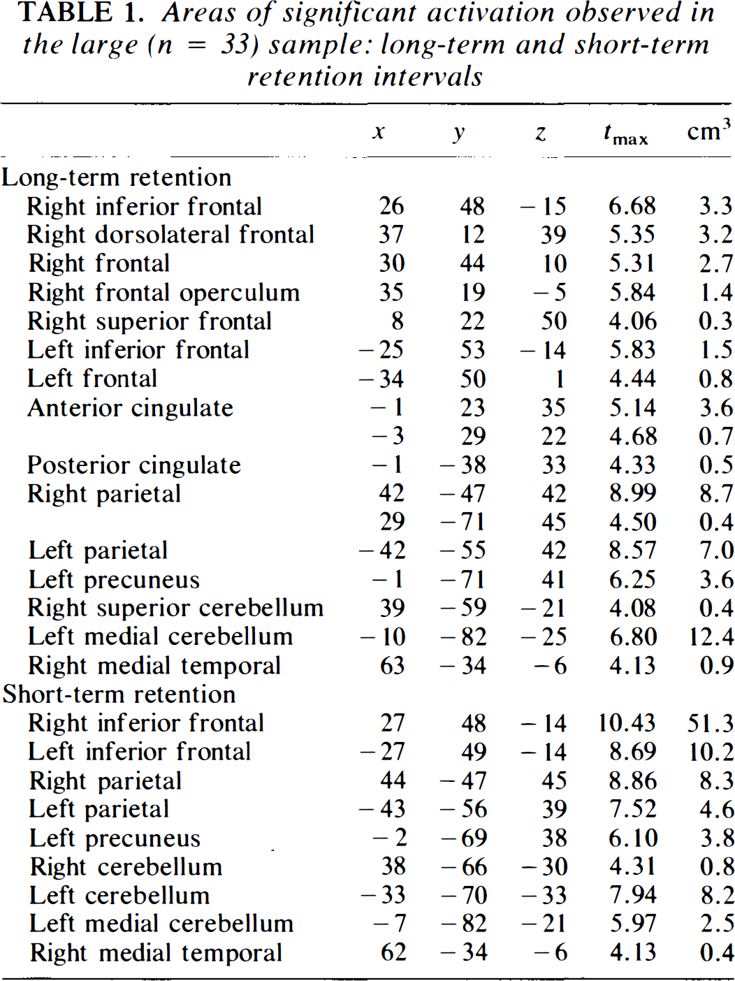
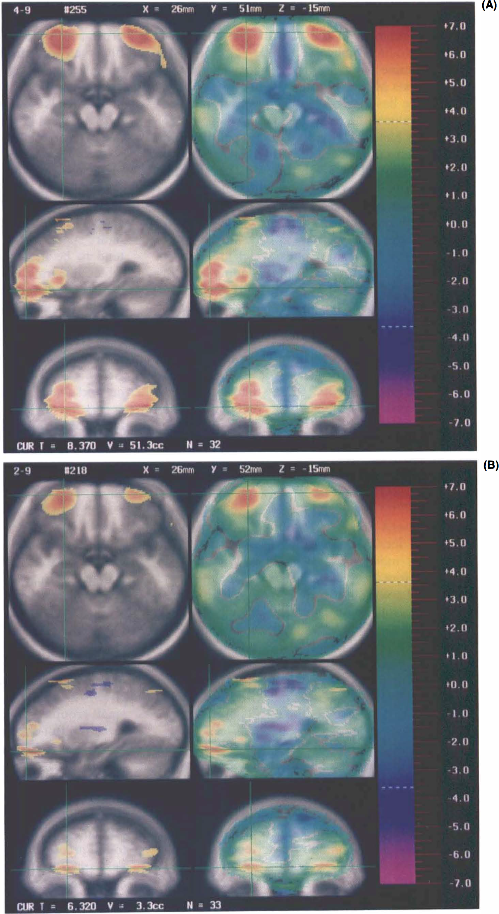
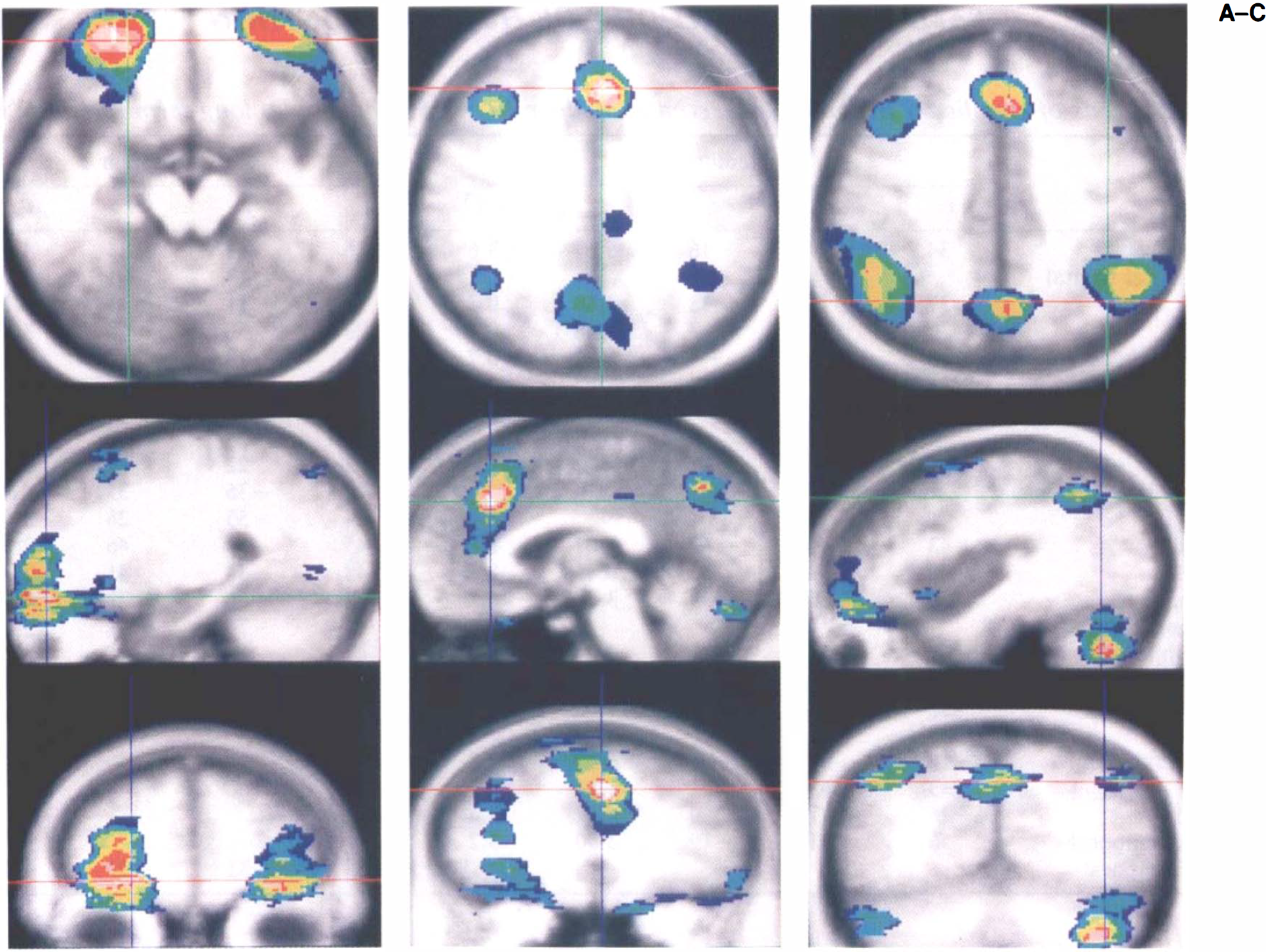
Two memory conditions were examined in this study: long-term retention with repeated practice and short-term retention with no practice tested 60 s after exposure to novel material. In a previous report, we have discussed the implications of the findings from this comparison, which were based on the analysis of the large (n = 33) sample (Andreasen et al., 1995). A more extensive summary of the results of this study, including all peaks composed of >50 pixels, is shown in Table 1. Some representative images, which illustrate the networks visualized, are shown in Fig. 1. As discussed in our original report of this study, we consider the findings to be consistent with the hemisphere-encoding/retrieval asymmetry model of memory proposed by Tulving et al. (1994b), which posits hemispheric asymmetry for encoding and retrieval. These results are also consistent with several other studies suggesting the importance of right frontal regions for retrieval and left frontal regions for encoding (Kapur et al., 1994; Shallice et al., 1994; Tulving et al., 1994a; Fletcher et al., 1995).
Areas of significant activation observed in the large (n = 33) sample: long-term and short-term retention intervals
The t statistic images for short-term
Effects of intensity of activation and interindividual variability
Various studies examining primary perceptual processes such as vision have shown that sensory stimuli can produce large changes in blood flow and activate regions that have minimal interindividual anatomic variability. For example, blood flow in primary visual cortex in response to a flashing checkerboard may increase as much as 40% (e.g., Hurtig et al., 1994). However, the intensity of activation in studies of more complex cognitive processes is probably lower, and intersubject variability is probably greater. These considerations will inevitably impinge on the size of the sample required to produce replicable results.
To determine the quantitative increase occurring in the regions affected by the memory tasks in relation to the baseline task, we measured the absolute flow values in a subset of selected regions of interest. As expected, the long-term condition produces smaller increases in flow than does the short-term condition. The magnitude of the increase ranges from a low of 3.9 (anterior cingulate for long-term) to a high of 13.3 (right frontal for short term). All of the increases in the well practiced and efficient long-term condition are <10%. In the short-term condition, the frontal lobes, which are presumably actively engaged in both encoding and retrieval, have the greatest increases and exceed 10%. Other things being equal, these should be the most reproducible regions to be detected as sample size decreases.
Individual variability in intrinsic brain anatomy produces another source of variance that can affect sample size requirements. Most studies employ a filter that smooths the images to “reduce anatomic variability” by blurring spatial locations. To obtain a perspective on the effects of anatomic variability, we calculated the means and standard deviations for normalized flow in the same regions without using the standard 18-mm filter. As anticipated, eliminating the filter increased the variance: The standard deviations are nearly double. However, the size of the increases in flow, as compared with baseline, is modestly greater in these unfiltered data. As before, increases are greater for the more difficult and novel short-term condition than for the long-term condition. Percentage increases range from 8 to 16.4. The large standard deviations suggest that interindividual variability is indeed a real occurrence, but the larger percentage increases produced by eliminating the filter suggest that filtering may reduce sensitivity to peak detection rather than enhance it. Further study of the effects of filtering is clearly needed.
Effects of sample size on identification of networks
The primary test of the smaller samples is the extent to which they replicate the networks observed in the large sample and in other studies of human memory. The most valid replication would identify the frontal asymmetry described previously and shown in Table 1, as well as the associated biparietal and left and right cerebellar activations. There is a well recognized anatomic cross-connectivity between frontal cortex and cerebellum (Schmahmann, 1991; Middleton and Strick, 1994). For these memory conditions, co-occurrence of cross-hemispheric frontal-cerebellar activation is observed with striking consistency. In addition, the cingulate is activated in both conditions (although it does not appear in Table 1 because the short-term activation is so large that the cingulate coalesces with adjacent cortical regions), and the left precuneus is also activated.
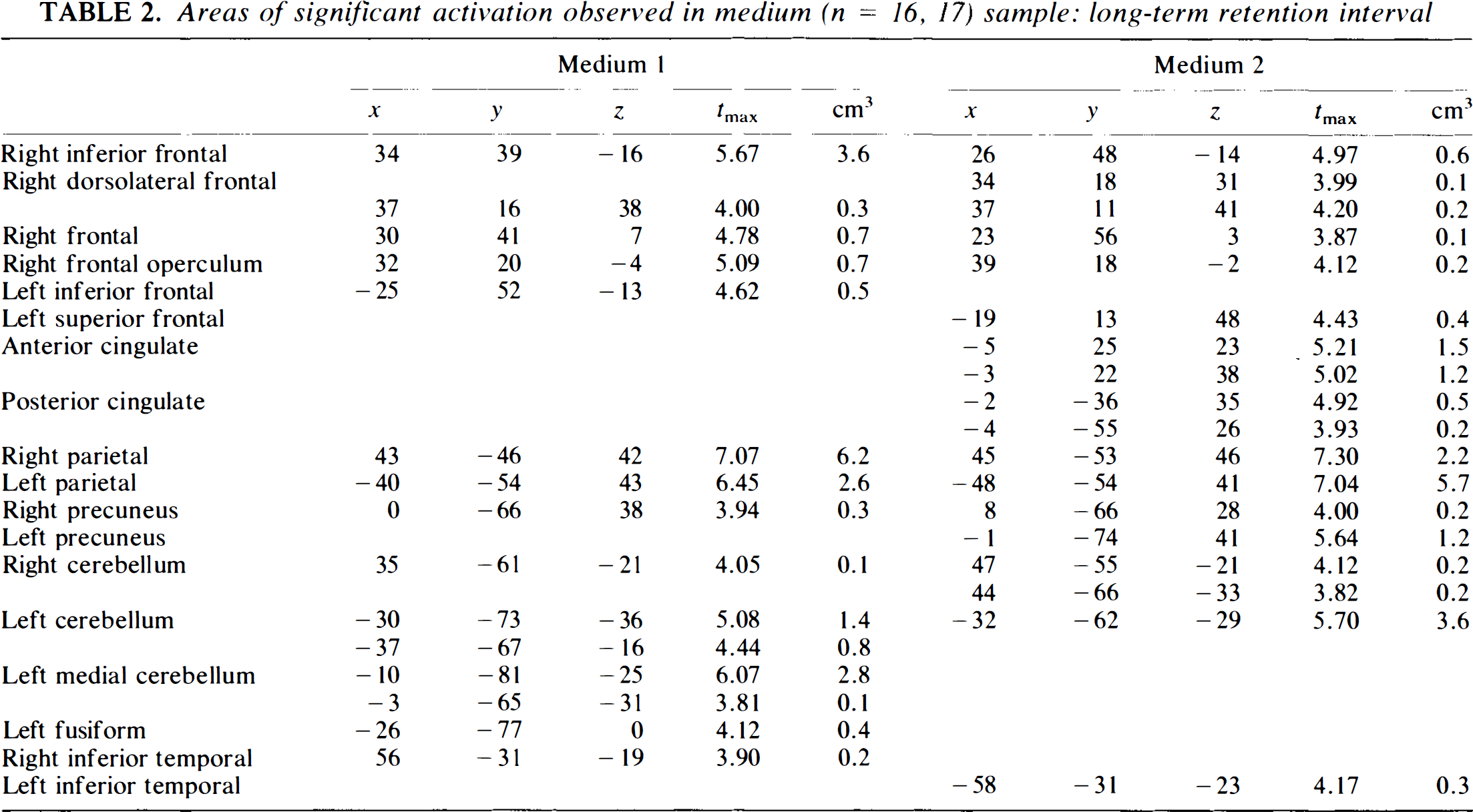
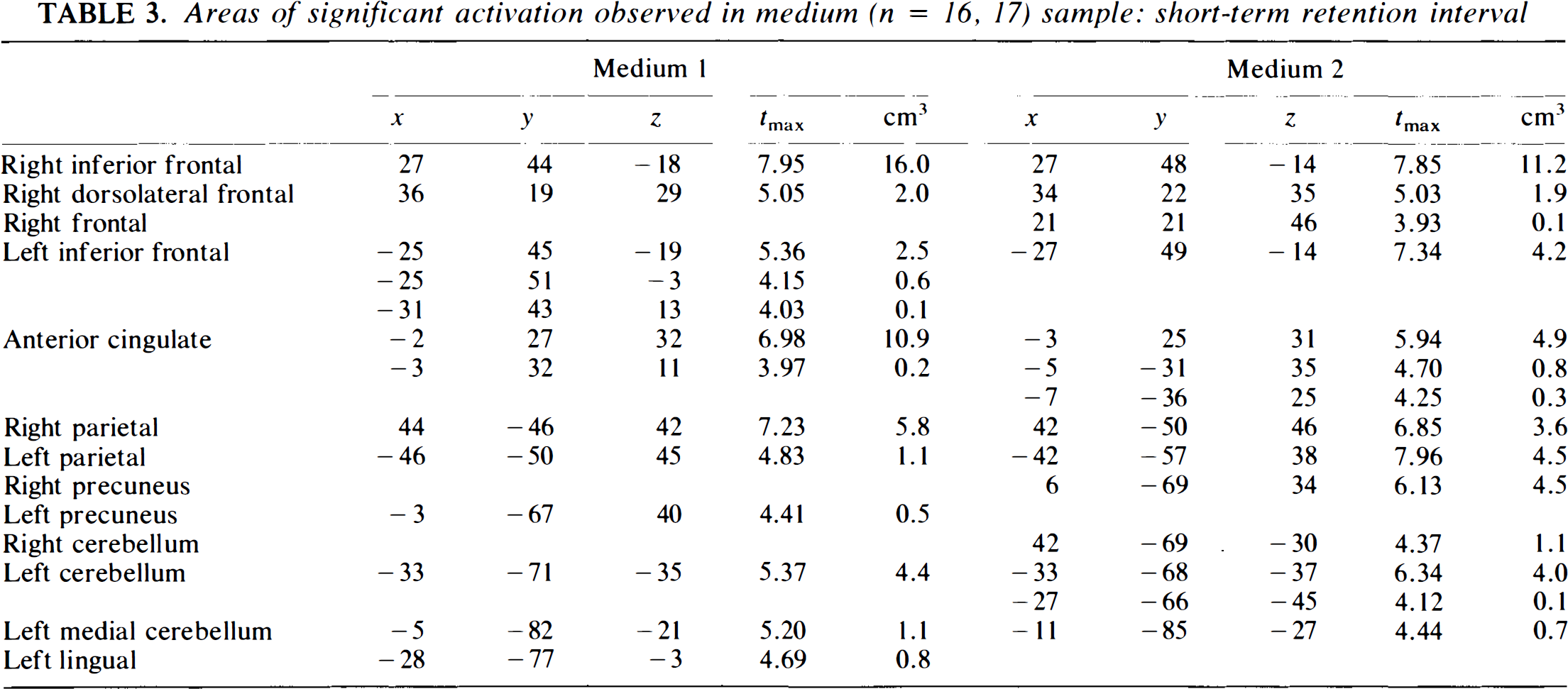
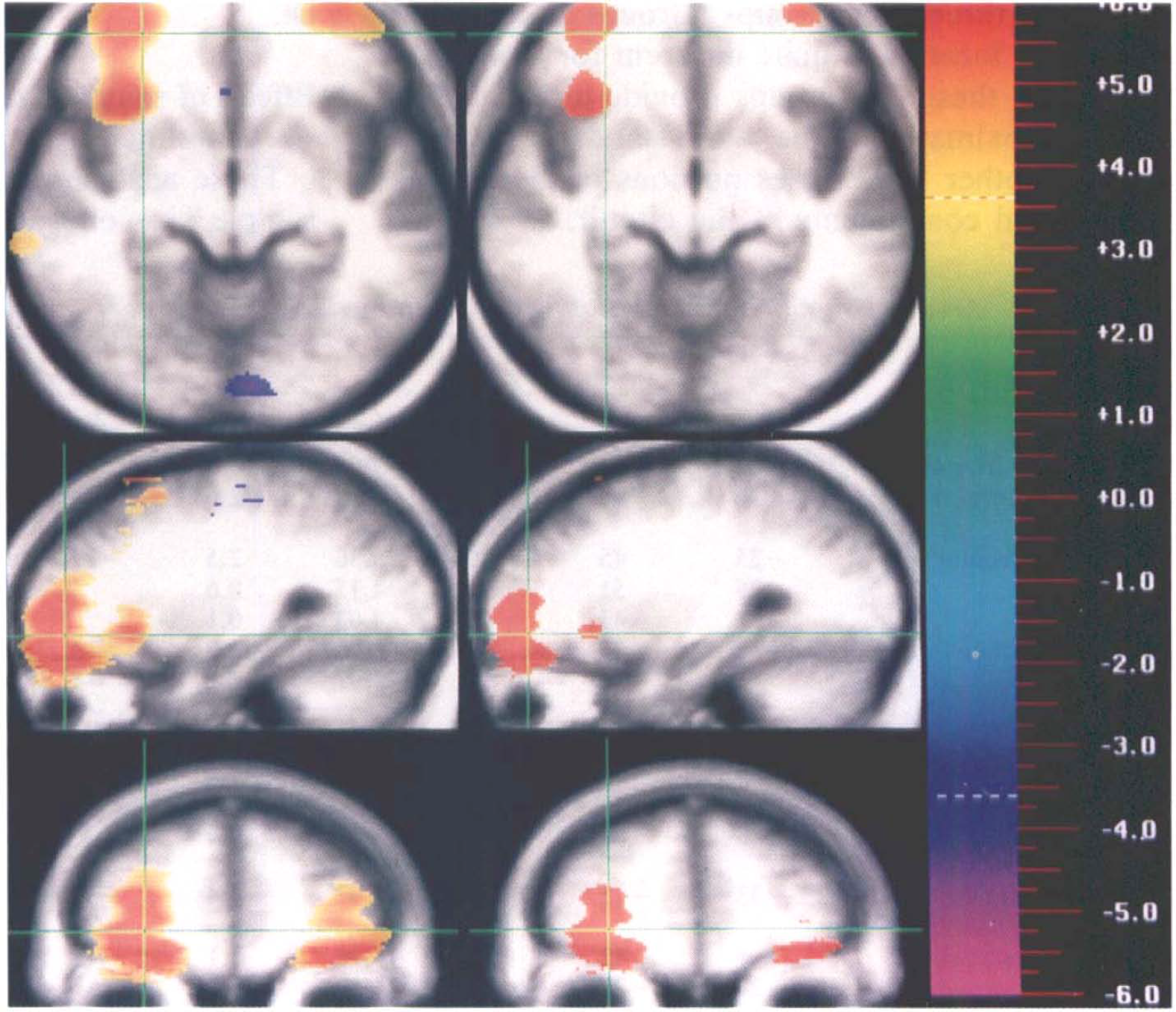
The results of the sample subdivision are shown in Tables 2–7. The conclusions are similar for both tasks. Figure 2 illustrates the findings visually. Here, the peaks from the various samples are shown as overlapping/superimposed images; as this figure suggests, the peaks from the smaller samples tend to be nested inside the larger samples. The tables illustrate these findings in more detail. The medium sample produces the closest replication of the large sample. For both conditions, the findings are nearly identical. For the long-term condition, both groups have similar peaks in all regions except for cingulate gyrus (present in Group 2 and not Group 1), and the peaks are also very similar to the networks seen in the large sample. A similar result occurs for the short-term condition, but in this case the results are virtually identical in the two medium samples and are also virtually identical to the large sample; this result probably reflects the fact that the short-term condition produced larger activations, often of higher intensity, and these were therefore less likely to get “lost” as the sample size (and resultant power) decreased.
Areas of significant activation observed in medium (n = 16, 17) sample: long-term retention interval
Areas of significant activation observed in medium (n = 16, 17) sample: short-term retention interval
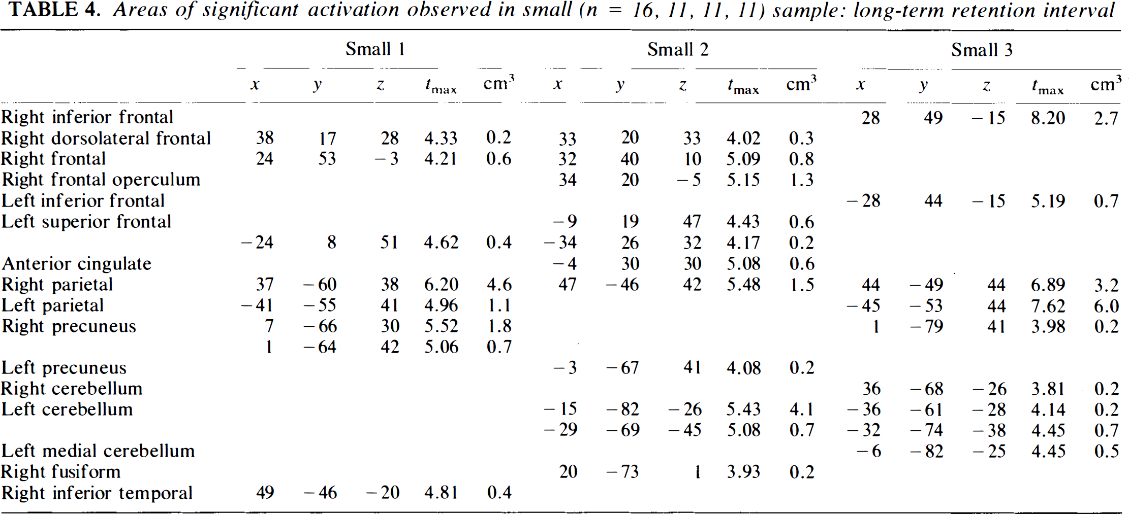
Areas of significant activation observed in small (n = 16, II, II, 11) sample: long-term retention interval
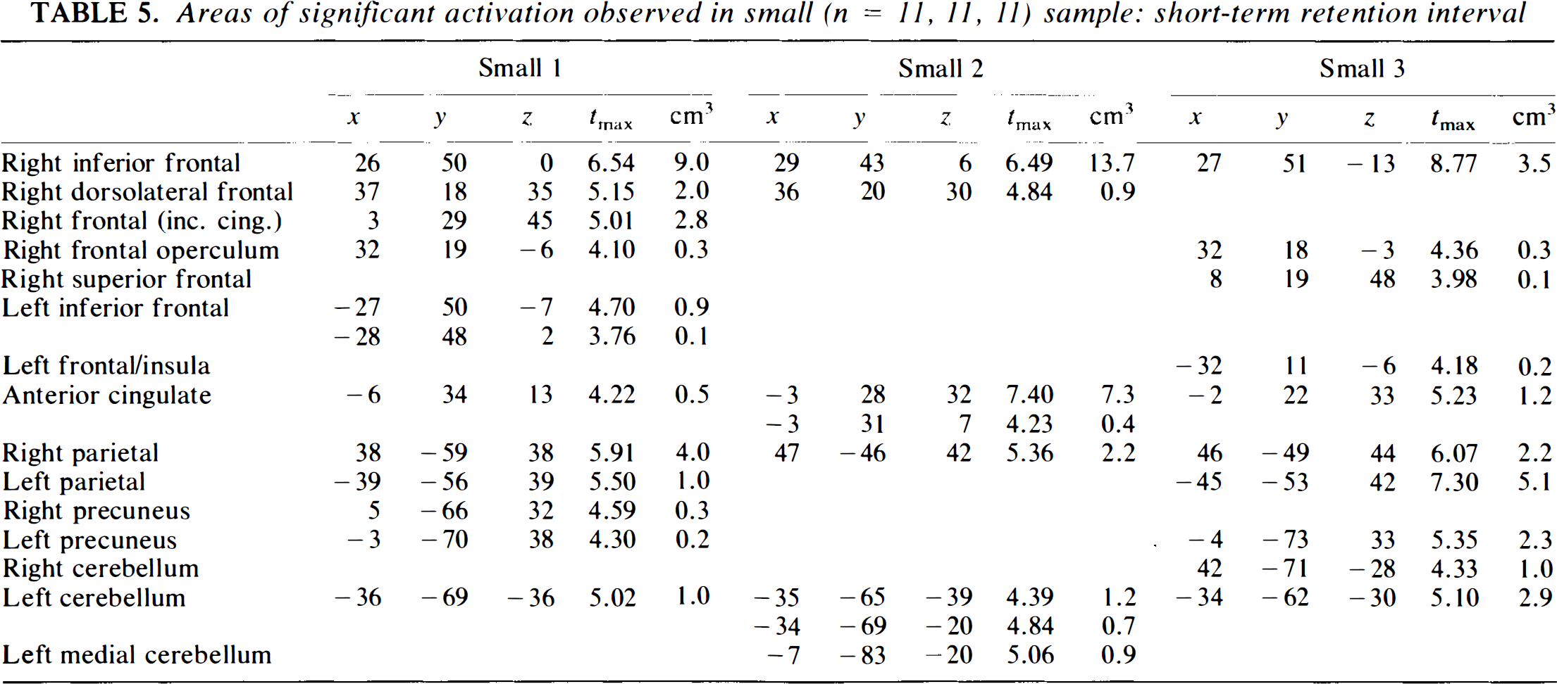
Areas of significant activation observed in small (n = 11, II, 11) sample: short-term retention interval
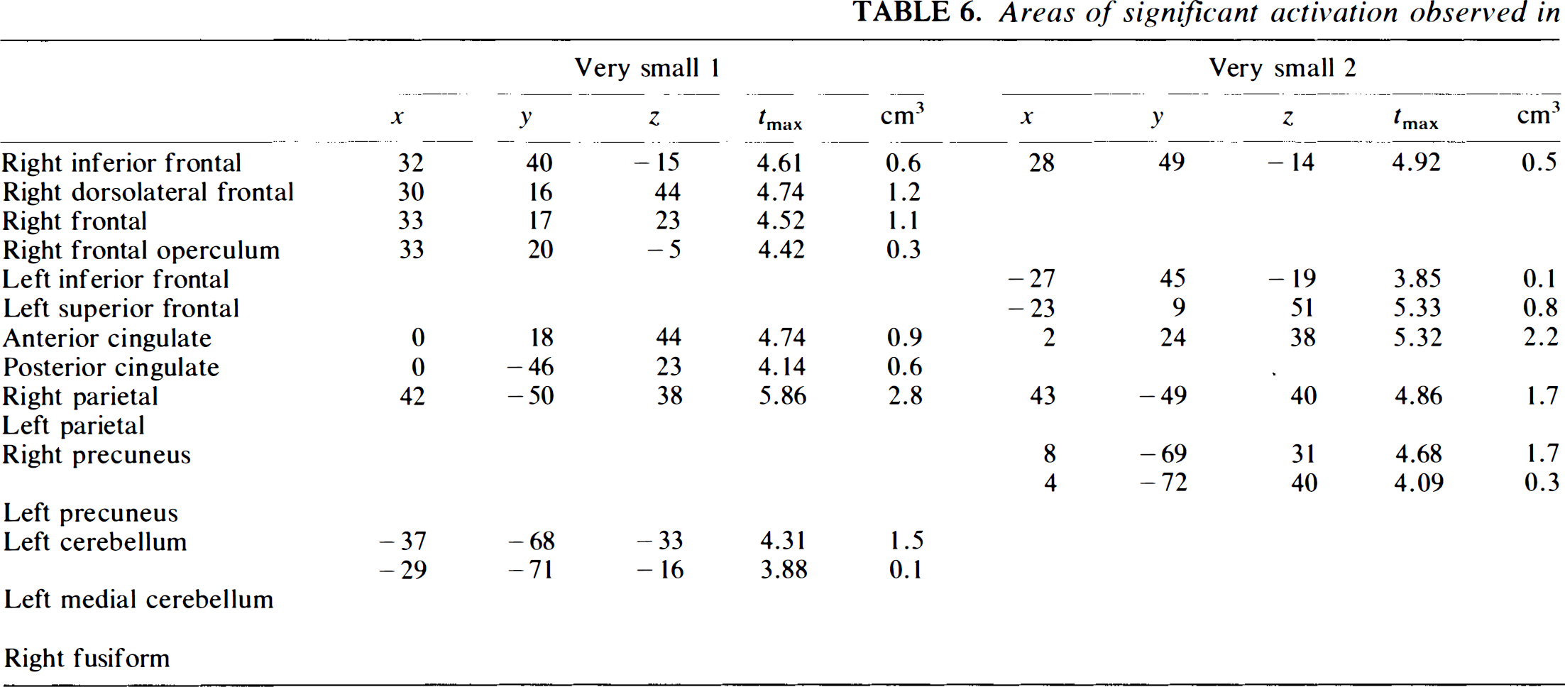
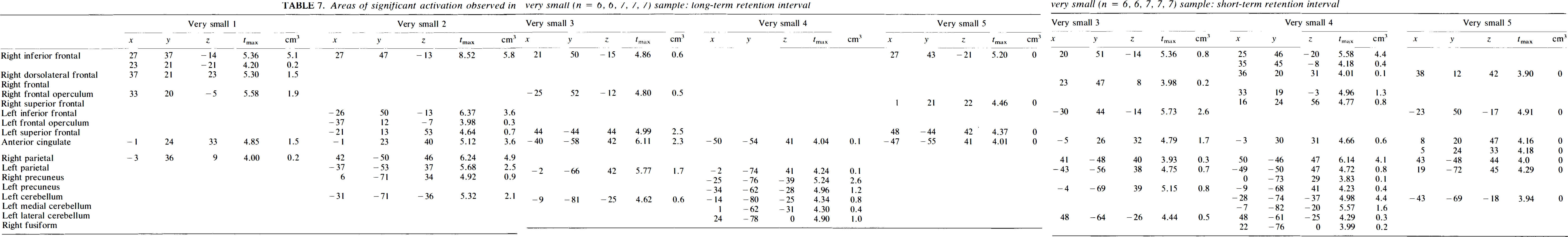
Areas of significant activation observed in very small (n = 6, 6, 7, 7, 7) sample: long-term retention interval
Areas of significant activation observed in very small (n = 6, 6, 7, 7, 7) sample: short-term retention interval
A Venn diagram illustrates how the peaks detected by the various sample sizes tend to be nested within one another, with the large sample detecting the largest number of activated pixels and with decreasing detection as sample size decreases. The overlap of pixels above the significance threshold for all subgroups is displayed as colored pixels ranging from dark blue (only one group with voxels above the threshold) to white (all groups with voxels above the threshold). This figure illustrates the data for the short-term retention interval at various locations in the brain; location of the three orthogonal planes
When the sample size is reduced to the small and very small sizes, more peaks begin to drop out. The problem is more severe for the long-term condition. For this condition, only one of the small groups (Group 3) identifies much of the network: right and left frontal regions, biparietal, and left and right cerebellar; however, it misses other components (cingulate, left precuneus). Group 1 loses the left cerebellum as well as the cingulate and precuneus, while Group 2 loses the left parietal region. The very small groups are very unstable. None of them captures the full circuit. Group 1 loses the left frontal and left parietal and precuneus, Group 2 the left parietal and cerebellum, Group 3 (the closest to large and medium) the cingulate, Group 4 the entire frontal component of the networks as well as the parietal components, and Group 5 much of the frontal and all of the cerebellar components in addition to the precuneus. Thus, only one of five among the very small groups could be considered to provide an adequate replication. Depending on the strictness of the criteria, only two or three of the small groups perform adequately.
The situation is slightly better for the short-term condition, which is potentially more robust to decreasing sample size, because the activations are larger and more intense. In this instance, the ability to detect the encoding function in the left frontal region is especially important, and it is identified by two of the three small groups (Groups 1 and 3, although the location is quite different for Group 3). In general, these two groups provide a reasonably close approximation to the “gold standard.” Group 2, on the other hand, loses portions of the frontal and parietal components of the circuit, as well as other regions. When the sample size drops to very small, three groups are able to replicate a right and left frontal, biparietal, and left cerebellar circuit (Groups 2, 3, and 4). Group 1 loses large posterior components, while Group 5 loses a parietal component and has a substantial diminution of peaks overall.
Effects of sample size on peak distances, number, size, and intensity
These analyses provide a view of the effects of sample size on pattern detection. An alternative perspective on the effects of sample size is provided by quantitatively examining the stability of peak location (distances), number, size (volume), and intensity (t value) as sample size decreases.
For these analyses, we used slightly different peak locations. Peaks identified through statistical analysis techniques such as the Montreal method or statistical parametric mapping will agglutinate or fragment depending on the level of significance that is selected to identify the presence of a peak (Arndt et al., 1995). The excursion areas identified using the 3.61 critical value were very large for a few peaks (e.g., right frontal region for the short-term condition); the analysis of the smaller groups, coupled with visual inspection of the t maps, indicated that such large areas could contain multiple smaller peaks. Repeating the data analysis with a 5.19 critical value (corresponding to a corrected p < 0.001 and a 600-cm3 search volume with 2.47-cm3 resels) broke up many of these large areas. Figure 3 illustrates the fragmentation of the large agglutinated right frontal peak when the critical value is increased. If several peaks appeared within an area when this more stringent critical value was employed, those peaks were used for the following analyses; however, if the higher critical value did not identify any embedded smaller peaks, then the locations from the previous analysis (critical value = 3.61) were used. With use of the combination of thresholds, the long-term memory condition provided vided 18 unique peak locations and the short-term condition provided 12.
It is shown how changing the critical value for detecting peaks can produce fragmentation or agglutination. The effect of increasing the t threshold from 3.61 (left side of figure) to 5.19 (right side of figure) is illustrated. The right frontal peak and the insular cortex peak are connected (i.e., agglutinate) at the lower threshold but separate (i.e., fragment) at the higher significance threshold.
Peak distances
The average vector distance between the peak for the large sample and the corresponding peak in each of the smaller samples is shown in Table 8. Based on statistical theory and assuming that the variability in each dimension is independent, increasing the sample size should improve the accuracy of the peak location as a function of the square root of the n. Thus, increasing a sample size from 6 to 11 should reduce the root mean square (RMS) peak distances by a factor of 0.74 (= 61/2/111/2). Increasing the sample size from 11 to 16 should further reduce the RMS distance by a factor of 0.83 (= 111/2/161/2). When this simple theoretical formulation is applied to the locations of peaks found by PET, many physical constraints are present, which make it an oversimplification. The RMS distances based on the different sample sizes show a loss of accuracy that is most noticeable from the medium (n = 16) to the small (n = 11) sizes. In the long-term condition, the average RMS distance for all peaks in the medium-sized (n = 16) samples was 7.84 mm. Reducing the sample size to 11 increased the mean RMS distance to 9.04. In the smallest sample, the average distance was slightly smaller (8.83). The short-term condition data showed a more dramatic reduction in location accuracy (RMS distances) from 4.07 mm in the medium-sized samples to 6.99 mm in the small samples. pies. Reducing the sample size further changed the average error less (RMS distance in the very small sample = 8.40).
Average vector distance (mm) between peaks detected in large sample and three smaller samples
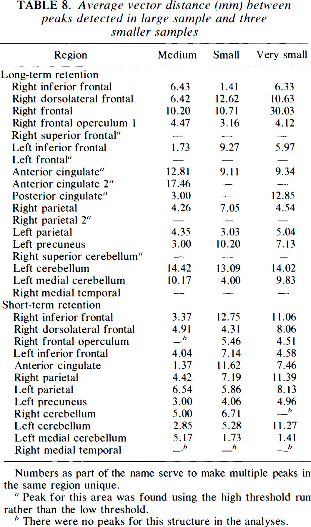
Numbers as part of the name serve to make multiple peaks in the same region unique.
Peak for this area was found using the high threshold run rather than the low threshold.
There were no peaks for this structure in the analyses.
Number of peaks
The number of peaks identified is directly affected by the fragmentation-agglutination problem referred to already. That is, the number of peaks detected is related to the significance threshold (critical value) selected, combined with the number of contiguous pixels and the number of spatially separated pixels with a high t intensity. Within the high threshold selected for quantitative analyses to reduce agglutination, however, on average the number of peaks decreased as the sample size decreased. In the long-term condition, the original large sample revealed 18 areas. For the medium, small, and very small samples, the mean numbers of peaks per analysis were 16.5, 9, and 6.6, respectively. The numbers of peaks were similarly arranged for the short-term condition. The medium sample found 13 peaks compared with 12 in the large sample. The small sample analyses found 9.67 peaks and the very small found 8.4 peaks on average.
The probability of finding a peak in a sample also decreases as the sample size goes down. For the long-term condition, the medium-sized sample had a 77% chance of identifying the original 18 peaks. For the small and very small samples, the percentages were 50 and 43, respectively. A similar pattern of decreasing peak detection with decreasing sample size was also apparent in the short-term condition. The chances of finding significant peaks were 90, 67, and 60% for the medium, small, and very small sample sizes, respectively. These numbers are somewhat lower than would be expected from formal power estimates. Most of the peak areas of activation produced very large t values, and consequently large effect sizes, so that power estimates are usually good (i.e., >0.9), even for the smallest samples.
Peak size and intensity
Peaks with a high intensity also tend to have a larger volume. In the large sample, peak size and intensity correlated 0.58 and 0.84 for the long- and short-term conditions. The relationship of intensity and size held up across the sample sizes. The relationships were closest for the larger sample sizes. For instance, the correlations of the large sample t value with the medium sample volumes were r = 0.72 and 0.79 for the long- and short term conditions, respectively. This relation weakened as the sample size went down, but was still reasonably strong for the small samples (r ∼0.6). The relationship was marginal for the smallest sample size (r ∼0.3). This suggests that volumes in the medium and small samples gave an indication of the size and intensity for the large sample, but that the very small samples were only weak indicators.
DISCUSSION
PET studies are expensive. Although expense is sometimes estimated in terms of the cost of obtaining imaging data, the real expense includes substantial indirect costs that increase exponentially. Recruiting subjects, documenting their cognitive and sociodemographic characteristics, designing the sequence of cognitive measures to be obtained, developing appropriate testing materials, purchasing and maintaining imaging equipment, exposing subjects to radiation and inconvenience or pain, obtaining MR data for image registration, maintaining and manipulating large data sets that include both imaging and clinical data, developing or acquiring software for sophisticated image analysis, performing steps in image analysis such as PET/MR registration, conducting complex statistical analyses, and interpreting the results of such analyses—all these necessary steps mean that each subject costs thousands of dollars. In this context, identifying the optimal size for a PET study of human cognition is important.
In this study, we have attempted to examine the criteria that can be applied to identify the appropriate sample size in PET studies. We have used a hierarchical approach that makes explicit the various criteria for evaluating the effects of reducing or increasing sample size and have explored their impact in a data set that could be used to determine the effect of using a very small (and therefore potentially very cost-effective) sample versus a larger (and therefore potentially more replicable and more generalizable) sample.
The results suggest that an optimal sample size for a PET study of cognition that produces small changes over baseline (between 4 and 13% in normalized filtered data) is between 10 and 20 subjects. The actual sample size needed will depend on the nature of the activation; if the change in flow over baseline is large, it will be detectable with smaller samples, while smaller and more subtle changes will require larger samples. In this particular study, samples of 16 and 17 produced results that were quite comparable with one another and with the original large sample that we studied for both the short-term and the long-term conditions. As sample size decreased, cross-sample replicability decreased as well. The samples of 11, 11, 11 were moderately stable, but the smaller samples of 6, 6, 7, 7, 7 were unstable, even for the large activations observed in frontal regions. The short-term condition, which produced higher percentage changes in flow over baseline, produced more consistent results with decreasing sample size than did the long-term condition. As is often the case, one must choose in which direction one wishes to err.
The results of this study suggest that the price of decreasing sample size involves primarily an increase in false negatives. As the sample size decreased, false positives usually did not emerge. This suggests that the exploratory statistical methods used for PET data analysis are relatively conservative and do not err by finding peaks that are not actually present. Instead, they err primarily by failing to find all the peaks that are present, particularly in small samples. The major loss was of regions that had a smaller volume and intensity of t value in larger samples. Consequently, investigators face a trade-off. If they wish to obtain a quick preview of some of the brain regions involved in a specific mental activity, they will find some of the regions with a small sample. They run the risk of missing other regions that may be equally important, however, and they probably will not be able to identify the full array of complex networks that is engaged in complicated mental operations such as encoding and retrieving information in the activity that we refer to as “memory.”
The analyses presented here appear to suggest that larger sample sizes are preferable. An important limitation of the current analysis, however, is that we investigated only a single measure of a cognitive condition. An alternative approach, not explored in the current study, is to obtain multiple measures of the same cognitive task within smaller samples; some investigators use this approach to study small samples with multiple repeats, based on the assumption that signal-to-noise ratio will be improved because intersubject variability will be reduced (e.g., Fletcher et al., 1995). The extreme case of this approach would involve intensive study of a single individual. This strategy is an alternative and potentially effective way to increase sample size without increasing the number of subjects. This strategy may have limitations in generalizability to larger and more diverse groups of individuals, however, and it also assumes that the response to the task remains the same across repetitions. The latter assumption is called into question by the various studies showing the effects on blood flow of both practice (Raichle et al., 1994; Andreasen et al., 1995) and novelty (Tulving et al., 1994c). Nonetheless, any conclusions concerning sample size that are drawn from this particular study can be applied only to studies in which conditions are not repeated and averaged. Studies that repeat conditions may successfully employ smaller samples. The advantages and disadvantages of using larger samples with single conditions versus smaller samples with repeated conditions require further empirical investigation.
For most analyses in this study, we have used a single fixed threshold for determining the presence of a peak (i.e., 3.61). This represents a corrected probability of ∼0.5 given our scanner parameters, smoothing, and the usual volume of gray matter in our subjects. Thus, one of two experiments might show at least one false peak above 3.61. Theoretically, the critical value (cutoff) of t tests will decrease as sample size increases; concomitantly, however, agglutination will also become a greater problem, and investigators will begin to miss peaks as they are subsumed or gobbled up by adjacent larger-valued peaks. This may be a case when the hypothesis-testing and exploratory strategies are at odds with one another. The value of placing primary emphasis on significance thresholds alone should be given careful consideration in exploratory PET studies; in most circumstances, other considerations should also be examined, such as size and location of peaks.
Accurate location may be more meaningful than the magnitude of the p value, once a minimal significance level is achieved. The sample size affects both indicators by increasing the power to detect a significant peak and by improving the accuracy of the peak's estimated location. There is a law of diminishing returns regarding sample size and the ability to pinpoint a peak's coordinates. The resolution afforded by the sample size must also be weighted by the physical constraints of the relevant anatomy and physiology. For some structures located among several possible candidate gray matter alternatives, such as two nearby gyri, a larger sample may be preferable. However, for other more isolated structures, surrounded by white matter or CSF, the location may require less accuracy and may be adequately estimated by a moderate-size n.
These results have implications for efforts to create a database that will permit merging of data across centers to conduct meta-analyses. Sample size should perhaps be weighted in some way so that results from a specific study can be assigned an appropriate reliability and validity. The margin of error for identifying the coordinates of an activation can have a high degree of error, and this error is increased as sample size decreases. Ideally, meta-analysis must be applied in sophisticated ways that include pattern and number of peaks in addition to peak location, since the long-term goal of cognitive PET studies is to identify the cognitive networks engaged in a variety of complex mental activities.
Footnotes
Acknowledgment:
This research was supported in part by NIMH grants MH31593, MH40856, and MH-CRC43271; a Research Scientist Award, MH00625; and an Established Investigator Award from NARSAD.