Sage Journals: Discover world-class research

Abstract

When used to measure blood flow in the brain, water leaves a residue in the vascular bed that influences the estimation of blood flow by current methods. To assess the magnitude of this influence, we developed a two-compartment model of blood flow with separate parameters for transport and vascular distribution of brain water. Maps of the water clearance, K₁ into brain tissue, separated from the circulation by a measurably resistant blood–brain barrier (BBB), were generated by time-weighted integration. Depending on the validity of the assumptions underlying the two-compartment model presented here, the maps revealed a significant overestimation of the clearance of water when the vascular residue was ignored. Maps of V_o the estimate of the apparent vascular distribution volume of tracer H₂¹⁵O, clearly revealed major cerebral arteries. Thus, we claim that the accumulation of radioactive water in brain tissue also reflects the volume of the arterial vascular bed of the brain.

Keywords

Cerebral blood flow Unidirectional clearance of water Unidirectional extraction Initial distribution volume Positron emission tomography

The present study was designed to reveal the magnitude of the residue of water left in the vascular bed of the brain during the water's circulation after a bolus injection. Identification of this residue was intended to provide the basis for a method permitting the correct measurement of the clearance of water from the circulation into brain tissue as a more faithful index of perfusion than those currently used.

The permeability of the blood–brain barrier (BBB) to water is of such magnitude that radioactive water is often used as a tracer to measure cerebral blood flow (CBF), e.g., by positron emission tomography (PET). The use is based on the assumption that the tracer is instantly distributed to brain tissue as a whole, allowing blood flow alone, rather than the combination of blood flow, BBB filtrational and diffusional permeability, and capillary surface areas, to determine the water uptake.

It is, nonetheless, doubtful that the permeability of the BBB to water is sufficient to exclude a measurable resistance to instantaneous distribution. Limited diffusibility of water in the BBB has been reported frequently (Eichung et al., 1974; Gjedde et al., 1975; Herscovitch et al., 1983b; Raichle et al., 1983). Koeppe et al. (1987) demonstrated a significant overestimation of water clearance when the transmitted (vascular) radioactivity is ignored. The degree of overestimation depended on the length of data accumulation used to study the water exchange.

Gambhir et al. (1987) formulated a two-compartment model to describe the uptake of H₂¹⁵O in brain, assuming that arterial H₂¹⁵O fails to dissolve instantly and uniformly in brain tissue. With this model, estimates of clearance and distribution of H₂¹⁵O depended less on the duration of the study. This two-compartment model was based on the concept of an apparent vascular distribution volume, V_o, which holds the fraction of the tracer transmitted through the capillary bed at a concentration equal to the concentration in arterial blood.

The reformulated two-compartment model introduced in the present study yields both the unidirectional clearance of water from blood to brain, K₁, and the apparent vascular distribution volume, V_o, of the tracer. It is, therefore, different from the two-compartment model of Gambhir et al. (1987). The introduction of V_o reveals that it is not the total vascular volume but a smaller fraction thereof that depends on the BBB permeability of the tracer. Brain maps of the water clearance, K₁, and water's vascular distribution volume, V_o, were created by time-weighted integration (Alpert et al., 1984; Ohta et al., 1992). For comparison, we also generated maps with the one-compartment method (Alpert et al., 1984; Carson et al., 1986; Kanno et al., 1987; Raichle et al., 1983), which has no vascular volume. The precision of this new method's use of three-parameter analysis by weighted integration was tested by simulation.

EXPERIMENTAL DESIGN AND THEORY

The basic design of the study included derivation of novel equations describing water accumulation in brain tissue and comparison of the results of PET studies using these novel equations with results obtained by conventional computational strategies.

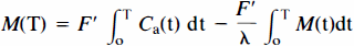
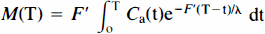
For the nonsteady-state, and with the assumption that larger vessels as well as exchange vessels may reside in the field of view of the tomograph, we derived the equation for the accumulation of inert tracer in a tissue (see Appendix for derivation of equations and Fig. 1 (left panel) and Table 1 for explanation of symbols):

TABLE 1.

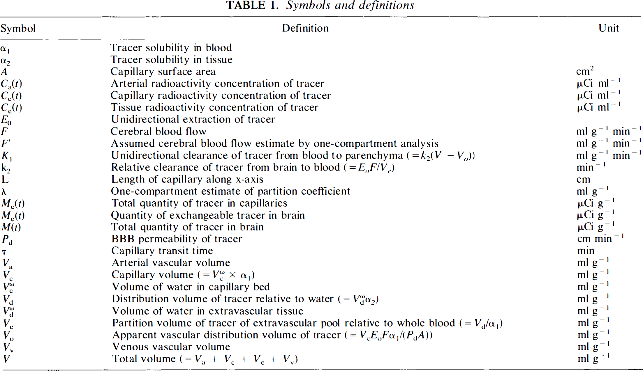
Symbols and definitions

Symbol	Definition	Unit
α₁	Tracer solubility in blood
α₂	Tracer solubility in tissue
A	Capillary surface area	cm²
C_a(t)	Arterial radioactivity concentration of tracer	μCi ml⁻¹
C_c(t)	Capillary radioactivity concentration of tracer	μCi ml⁻¹
C_e(t)	Tissue radioactivity concentration of tracer	μCi ml⁻¹
E _o	Unidirectional extraction of tracer
F	Cerebral blood flow	ml g⁻¹ min⁻¹
F′	Assumed cerebral blood flow estimate by one-compartment analysis	ml g⁻¹ min⁻¹
K ₁	Unidirectional clearance of tracer from blood to parenchyma (= k₂(V — V_o))	ml g⁻¹ min⁻¹
k₂	Relative clearance of tracer from brain to blood (= E_oF/V_c)	min⁻
L	Length of capillary along x-axis	cm
λ	One-compartment estimate of partition coefficient	ml g⁻¹
M_c(t)	Total quantity of tracer in capillaries	μCi g⁻¹
M_c(t)	Quantity of exchangeable tracer in brain	μCi g⁻¹
M(t)	Total quantity of tracer in brain	μCi g⁻¹
P _d	BBB permeability of tracer	cm min⁻¹
τ	Capillary transit time	min
V _a	Arterial vascular volume	ml g⁻¹
V _c	Capillary volume (= V_c^ω × α₁)	ml g⁻¹
V _c ^ω	Volume of water in capillary bed	ml g⁻¹
V _d	Distribution volume of tracer relative to water (= V_c^ωα₂)	ml g⁻¹
V _d ^ω	Volume of water in extravascular tissue	ml g⁻¹
V _c	Partition volume of tracer of extravascular pool relative to whole blood (= V_d/α₁)	ml g⁻¹
V_o	Apparent vascular distribution volume of tracer (= V_cE_oFα₁/(P_dA))	ml g⁻¹
V _v	Venous vascular volume	ml g⁻¹
V	Total volume (= V_a + V_c + V_c + V_v)	ml g⁻¹

\frac{dM}{dt} = V_{o} \frac{d C_{a}}{dt} + (K_{1} + k_{2} V_{o}) C_{a} - k_{2} M

(1)

FIG. 1.

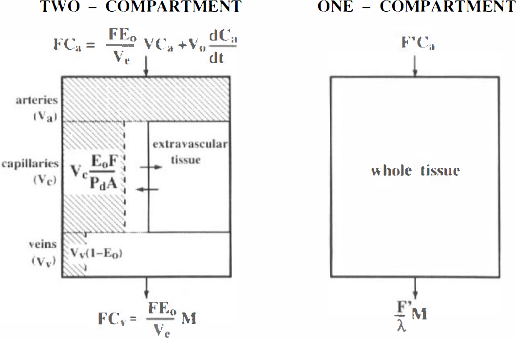
Two model configurations for the H₂¹⁵O PET studies. Two-compartment model for water clearance and apparent vascular distribution volume, V_o, (left, shaded area) and one-compartment model for blood flow (right). Note that for E_o→ 0, E_oF→P and V_cE_oF/P→V_c, and V_v (1 — E_o)→V_v, such that V_o→V_a +V_c + V_v. For E_a → 1,P >> F, therefore V_cE_oF/P→0, and V_v(1 — E_o) → 0, such that V_o → V_a.

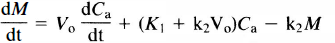
where M is the tracer quantity in brain and C_a the arterial concentration of the tracer. The three parameters, K₁, k₂, and V_o, were defined as follows: K₁ is the unidirectional clearance of water and k₂ is the rate constant of water removal from brain tissue. The term clearance is used with its conventional meaning of fraction of plasma water flow cleared of radioactive water, as derived below. V_o is a subvolume of the arterial (V_a), capillary (V_c), and venous (V_v) vascular beds; its magnitude depends on the permeability of the tracer. Definitions are shown in Table 1. The two solutions of Eq. 1 used in this work are

\begin{array}{l} M (T) & = & (K_{1} + k_{2} V_{o}) \int_{o}^{T} C_{a} (t) dt - k_{2} \int_{o}^{T} M (t) dt \\ +_{Vo}_{Ca} (T) \end{array}

(2)

and

M (T) = K_{1} \int_{o}^{T} C_{a} (t) e^{- k_{2} (T - t)} dt +_{Vo}_{Ca} (T)

(3)

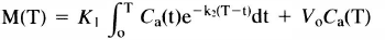
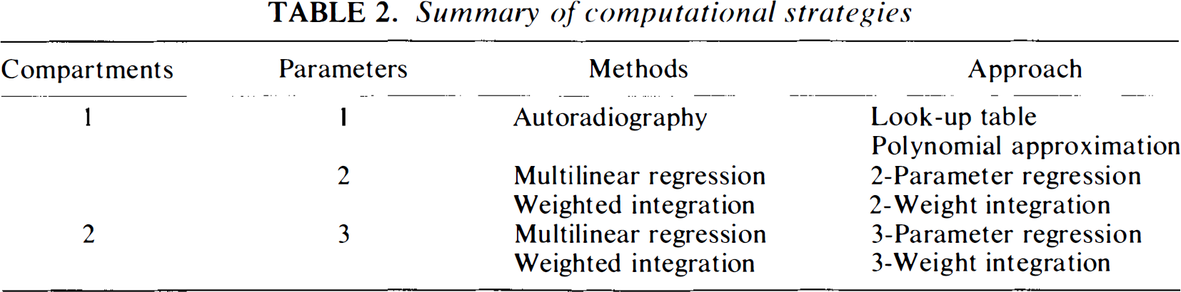
From these expressions, K₁, k₂, and V_o were estimated by multilinear regression (Eq. 2) or weighted integration (Eq. 3), as outlined in Table 2, which is a summary of computation strategies.

TABLE 2.

Summary of computational strategies

Compartments	Parameters	Methods	Approach
1	1	Autoradiography	Look-up table Polynomial approximation
	2	Multilinear regression	2-Parameter regression
		Weighted integration	2-Weight integration
2	3	Multilinear regression	3-Parameter regression
		Weighted integration	3-Weight integration

For comparison, we used the simplified bloodflow solutions derived in the theory section on one-compartment analysis to obtain single-compartment estimates of perfusion and partition coefficient

M (T) = F^{'} \int_{o}^{T} C_{a} (t) dt - \frac{F^{'}}{λ} \int_{o}^{T} M (t) dt

(4)

and

M (T) = F^{'} \int_{o}^{T} C_{a} (t) e^{- F^{'} (T - t) / λ} dt

(5)

where F′ and λ are the single-compartment estimates of perfusion and partition coefficient. The comparison was used to reveal and interpret the discrepancy between K₁ and F′.

The two compartments have three parameters (Fig. 1, left panel) that must be estimated by linear or nonlinear regression, or by weighted integration, as in the case of two parameters. The three parameters are either K₁ [= k₂(V — V_o], k₂(= F E_o/V_e) and V_o (shaded area), or k₂, V, and V_o. We expanded the two-weight integration to the estimation of three parameters, the three-weight integration, as described in the Appendix.

The single compartment has two parameters (Fig. 1, right panel), apparent blood flow, F′, and partition coefficient, λ. The two parameters were determined either simultaneously (two-parameter analysis) or apparent blood flow was calculated with an assumed fixed value of the partition coefficient (one-parameter analysis). The two-parameter analysis can proceed either by linear or nonlinear regression, or by weighted integration (Alpert et al., 1984; Carson et al., 1986; Koeppe et al., 1985). The one-parameter analysis is known as the ‘autoradiographic’ method because it mimics autoradiography in which a single measurement of the dependent variable is available (Kanno et al., 1987; Raichle et al., 1983).

METHODS

Simulated PET studies

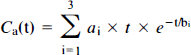
We evaluated errors in the time-weighted integration caused by tissue heterogeneity, tracer delay and dispersion of the peripherally sampled arterial input function, C_a(t). For this purpose, a typical input function, C_a(t), was first generated from the sum of three time-weighted exponentials (Herscovitch et al., 1983b),

C_{a} (t) = \sum_{i = 1}^{3} a_{i} \times t \times e^{- t / b_{i}}

(6)

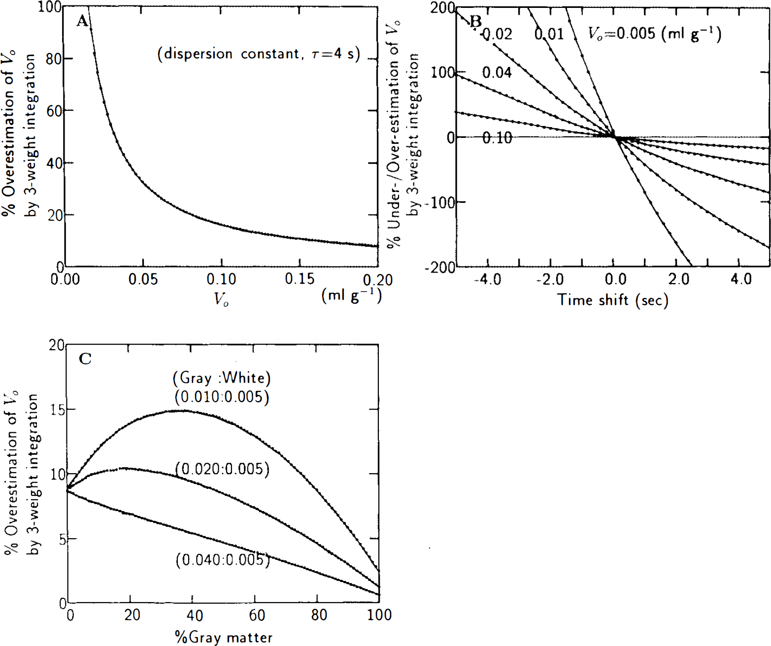
The effects of tissue heterogeneity, tracer dispersion and delay on the estimation of K₁ and V_o by three-weight integration were evaluated as outlined by Herscovitch et al. (1983b), Iida et al. (1986), and Meyer (1989). Tissue heterogeneity was simulated using Eq 4 with gray-white matter K₁ pairs of 0.4 and 0.2, 0.6 and 0.2, and 0.8 and 0.2 ml min⁻¹ g⁻¹ and V_o pairs of 0.010 and 0.005, 0.020 and 0.005, and 0.040 and 0.005 ml g⁻¹. These values were assumed to cover the realistically expected range for the two parameters. The K₁/k₂ ratio was always fixed at 0.9 ml g⁻¹. The accuracy of the three-weight integration was assessed by analysis of simulated data with superimposed random Poisson variability. First, uniform randomly distributed 5% Poisson noise was imposed on each point of the simulated input function. This variation was consistent with the error inherent in the manually sampled blood curves, including statistical variation and errors due to sample timing and weighing. Next, tissue time-activity curves were generated according to Eq. 3 with a 5-s sampling interval for a total length of 3 min, using the previously generated input function and selected values for K₁, k₂, and V_o. Uniform 5% Poisson distributed variability (P_N), approximately corresponding to that observed on real time-activity curves for 2-cm diameter regions of interest (ROIs), was imposed on each point of a given tissue time-activity curve using the equation

\frac{σ_{i}}{N_{i}} = \frac{p_{N}}{100} \times \sqrt{\frac{N_{m}}{N_{i}}}

(7)

Here, σ_i is the standard deviation of the Poisson variability added to the ith scan, N_i the individual counts in the ith scan, and N_m the mean frame counts corresponding to a 4-cm² region and 10⁶ total counts/plane in 3 min (Evans et al., 1986). K₁, k₂, and V_o were then estimated by the three-weight integration from simulated variable tissue and arterial time-activity curves. The accuracy of each of the three parameter estimates was expressed as the fractional root-mean-squared error (ε) for N = 100 variable patterns of each simulation,

ε = \frac{1}{p} \sqrt{\frac{\sum_{i = 1}^{N} {(p_{i} - p)}^{2}}{N - 1}}

(8)

where p_i is the parameter estimate and p its input value.

Human studies

Fifteen ‘dynamic’ (multiframe) H₂¹⁵O sessions were completed in nine young volunteers. Four subjects were studied both under normoventilation (average P_aco₂ 39.6 mmHg) and under hyperventilation (average P_aco₂ 23.0 mmHg). Six subjects were scanned with the Positome IIIp, a two-ring (BGO) Bi₄Ge₃O₁₂ head tomograph with transverse and axial spatial resolutions of 11 and 16 mm full width at half maximum (FWHM), respectively, and an interplane separation of 18 mm (Thompson et al., 1986). Three subjects were scanned with the PC-2048 15B (Scanditronix), an eight-ring BGO head tomograph with transverse and axial resolutions of ∼6 mm FWHM and an interslice separation of 6.5 mm (Evans et al., 1991). Reconstruction software on the Positome IIIp included corrections for detector efficiency variations, random events, a deconvolution procedure to eliminate scattered events (Cooke et al., 1984), and attenuation correction with a projection contour finding method. On the PC-2048 15B, similar corrections were applied, except for attenuation correction, which was performed with a rotating Ge-68 transmission rod source. Radioactive water was prepared with a Japanese Steel Works (Muroran, Japan) Medical Cyclotron (BC-107).

After completion of a questionnaire designed to exclude volunteers with neurological deficits, informed consent was obtained from each participant. The protocol was approved by the Research and Ethics Committee of the Montreal Neurological Hospital and Institute. Subjects' heads were immobilized by means of a customized self-inflating foam headrest. A short indwelling catheter was placed into the left radial artery for blood sampling and blood gas determinations.

The tracer H₂¹⁵O was injected as a bolus into the brachial vein of the right arm (20 mCi for Positome IIIp, 40 mCi for PC-2048 15B). Arterial blood sampling and dynamic imaging began at injection time. The flow of blood from the freely-flowing arterial sampling catheter was kept ∼10–15 ml min⁻¹ in order to minimize dispersion effects (Iida et al., 1986; Meyer, 1989). Dynamic scans with frame durations of 3 (Positome IIIp) or 5 s (PC–2048 15 B) were obtained over a period of 3 min and corrected for decay according to the method of Raichle et al. (1983). Blood samples were collected manually at ∼5-s intervals and assayed in a calibrated well-counter. As the sensitivity of K₁ to tracer dispersion and delay was expected to be minimal, as revealed by simulations (Ohta et al., 1992), the difference in tracer arrival between the brain and the peripheral sampling site was corrected by the simple slope method (Herscovitch et al., 1983b; Meyer, 1989), and dispersion, already minimized by the relatively large flow rate in the arterial sampling catheter, was not accounted for. Maps of V_o were generated under the same conditions. However, it was expected that V_o, as any purely intravascular component, would be extremely sensitive to the latter two effects. This sensitivity of V_o to errors in tracer dispersion and delay was confirmed by means of simulations. In four studies, tracer dispersion and delay were, therefore, carefully corrected, as outlined by Iida et al. (Iida et al., 1989), and adapted to our model with inclusion of V_o (Fujita et al., 1992). From these four studies, V_o values were derived, although quantification of this parameter was not the primary objective of this study. A dispersion time constant of τ = 4 s was used. K₁ and V_o values were determined for circular ROIs, each with an area of 3.7 cm², which were evenly placed over two brain slices (20 ROIs per slice) situated ∼40 mm above the orbitomeatal (OM)-line. Care was taken to avoid ventricular space as well as larger vessels.

[C¹⁵]O and [¹⁵O]O₂ were used in one subject to compare the CO-derived steady-state vascular volume (reflecting the total vascular volume) and the O₂-derived apparent vascular volume (expected to reflect mainly the arterial plus part of the venous volume) with the H₂O-derived apparent vascular volume (expected to reflect mainly the arterial volume), in order to test the validity of the numerical values provided by the corresponding V_o maps.

[¹⁵O]O₂ was administered by bolus inhalation and [C¹⁵]O by continuous inhalation for 2 min (Grubb et al., 1978; Meyer et al., 1987).

Each subject underwent a magnetic resonance (MR) scan (Phillips Gyroscan 1.5 Tesla superconducting magnet system; Best, Holland). MR images (MRIs) were coregistered with PET images to corresponding imaging planes by means of a procedure developed by Evans et al. (1989).

Data analysis

From the dynamic PET data, which had a reconstructed spatial resolution of 10 mm FWHM, we generated 388 tissue time-activity records from circular ROIs, each with an area of 3.7 cm², uniformly distributed over the entire area of the selected brain slices. From 15 bolus H₂¹⁵O studies, 289 curves were obtained from normocapnic studies and 99 from hypocapnic studies. Blood flow was calculated using one-compartment analyses, which included two-parameter regression, two-weight integration, look-up table, and polynominal approximation methods. For the latter two methods, a tissue-blood partition coefficient of 0.9 ml g⁻¹ and 60 s of data were used.

The clearance of H₂¹⁵O, K₁, and the apparent vascular distribution volume, V_o, were calculated by three-parameter regression and three-weight integration, both based on two-compartment analysis. The three-weighted integration is computationally more demanding than is the two-weight integration, but yields 128 × 128 pixel maps of K₁, k₂, and V_o in 1.5 min with a Microvax III (Ohta et al., 1992).

For all regression analyses, a 3-min data segment was used. Functional images were processed with a nine-point smoothing filter. Despite the relatively large ROI size, tissue-heterogeneity effects were not expected to significantly affect K₁ estimates, as suggested by simulation (Ohta et al., 1992). Images of V_o were merged with corresponding MRIs for ease of analysis and interpretation.

RESULTS

Simulated PET studies

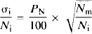
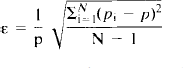
Simulated PET studies confirmed that the three-parameter analysis by weighted integration, in theory, yields precise estimates of apparent water clearance, K₁ (Fig. 2A). The fractional root-mean-squared (RMS) error inherent in the k₂ and V_o estimates by three-weight integration, with 5% Poisson variability added to both arterial and tissue radioactivity, increased markedly for small values of k₂ and V_o (Fig. 2 B,C). However, the error in K₁ was never >5%. K₁ was also relatively insensitive to dispersion effects of the arterial input function (Fig. 3A), arrival time difference of tracer between sampled site and brain (Fig. 3B), and tissue heterogeneity (Fig. 3C) (Herscovitch et al., 1983a; Iida et al., 1986; Kanno et al., 1987; Meyer, 1989). V_o, on the other hand, was extremely sensitive to systematic errors of tracer dispersion and arrival time estimates (Fig. 4A,B), while being moderately affected by tissue heterogeneity (Fig. 4C). Underestimation of the magnitude of any one of these three factors tended to elevate the estimate of V_o, to account for the presence of otherwise unexplained radioactivity in the tissue.

FIG. 2.

Root-mean-squared (RMS) errors of K₁, k₂, and V_o estimates determined by the three-weight integration after superposition of 5% statistical variability onto the arterial and tissue records.

FIG. 3.

A: Effect of dispersed arterial input function on K₁ estimate by three-weight integration. B: Effect of arrival time difference of tracer between peripherally sampled site and brain on K₁ estimate by three-weight integration. Positive time shift indicates delay of tracer arrival at arterial ‘sampling site’ relative to brain. C: Effect of tissue heterogeneity on K₁ estimate by three-weight integration for various gray: white ratios of tissue composition and K₁.

FIG. 4.

A: Effect of dispersed arterial input function on V_o estimate by three-weight integration. B: Effect of arrival time difference of tracer between peripheral sampling site and brain on V_o estimate by three-weight integration. Positive time shift indicates delay of tracer arrival at arterial ‘sampling site’ relative to brain. C: Effect of tissue heterogeneity on V_o estimate by three-weight integration.

Human studies

The real PET studies showed that F′ estimates always exceed K₁ estimates. By F′, we denote the value of K₁ estimated by means of the simplified single compartment model. Values of F′ (”blood flow”) calculated on the basis of the one-compartment analyses [two-parameter regression (Fig. 5A), two-weight integration (Fig. 5B), look-up table (Fig. 5C), and polynominal approximation (Fig. 5D)] were compared with values of K₁ obtained by the two-compartment model. Calculations were performed for a total of 388 regions in nine subjects. As expected, the discrepancy between F′ and K₁ markedly increased for larger values of the water clearance, K₁. This overestimation of K₁ by the single-compartment approach increased when V_o increased (Fig. 6). The degree of overestimation was positively correlated to the size of V_o.

FIG. 5.

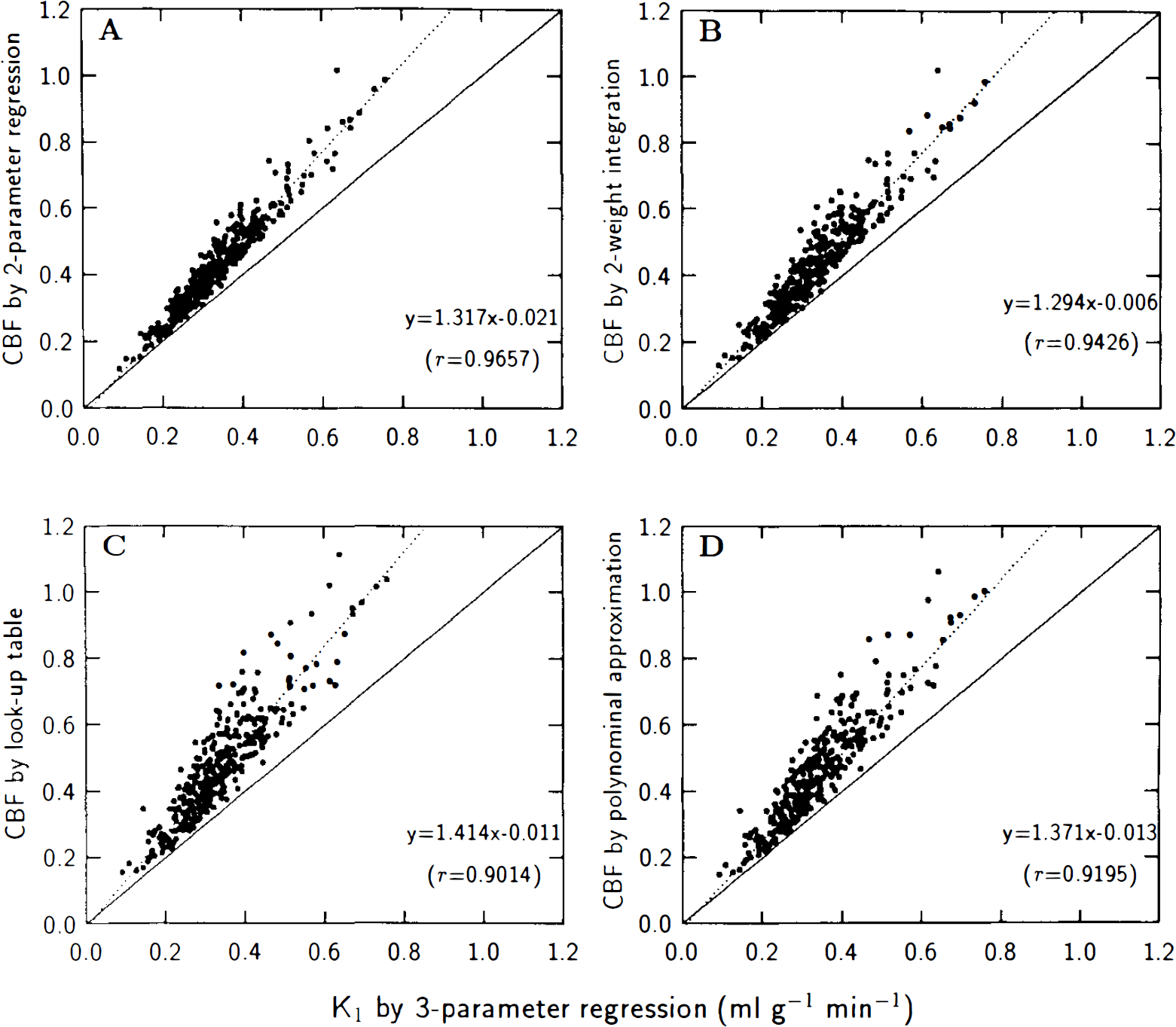
Water clearance, K₁, calculated by three-parameter regression, compared with F′ calculated according to one-compartment model, using in turn two-parameter regression, two-weight integration, look-up table, and polynominal approximation methods. The slopes of regression lines significantly exceeded unity (n = 388, p < 0.001).

FIG. 6.

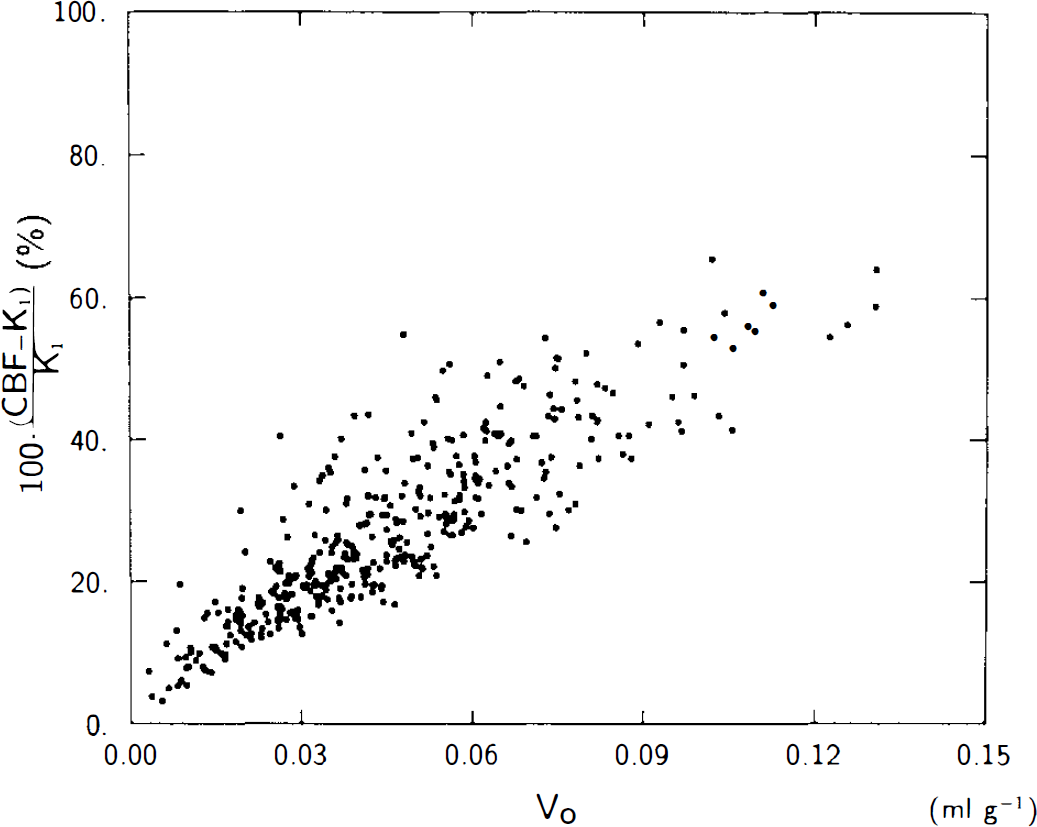
Percentage overestimation of F′ calculated by two-parameter regression, relative to water clearance, K₁, calculated by three-parameter regression, versus apparent vascular distribution volume, V_o, obtained by three-parameter regression. Note significant linear relationship between variables (n = 388, y = 454.43x + 6.7, r = 0.8552, p < 0.005).

Estimates of K₁ were considerably less time-dependent than those of F′ as evidenced by the calculated mean values and standard deviations of F′ and K₁ for the 289 normocapnic ROIs as a function of integration time (Fig. 7). Figure 8 illustrates the tissue time-activity curves predicted by the one-and two-compartment models. The two-compartment model (three-weight integration) described the observed data (black dots) well over the entire observation interval, in contrast to the one-compartment analyses (autoradiography and two-weight integration), which did not. Since tissue heterogeneity effects are not only minimal but very similar for the one- and two-compartment models (Fig. 3C and Fig. 4 in Ohta et al., 1992), we have used tissue data from an entire brain slice, which presents a lower noise level and, therefore, gives a clearer picture of the goodness of the various fitted curves. The result strongly validates the two-compartment model and its K₁ estimates.

FIG. 7.

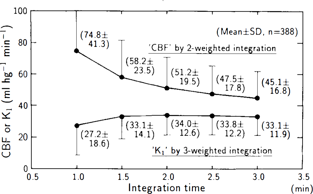
Mean and standard deviation of F′, for all regions at normocapnia, calculated by two-weight integration, and K₁ calculated by three-weight integration, as function of data collection (integration) time. Dots and vertical bars represent mean value and standard deviation, respectively.

FIG. 8.

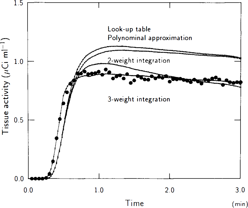
Single-plane H₂¹⁵O tissue time-activity record (dots), compared with record predicted by methods based on one-or two-compartment models. Note excellent fit obtained with three-weight integration (two-compartment) method.

Mean values and standard deviations of F′ and K₁ are summarized in Table 3. F′ estimates were close to accepted average CBF values (Lassen, 1985), but significantly larger than estimates of K₁ by two-compartment analysis (p < 0.001). Table 4 lists values of F′/λ and k₂, the values from the one-compartment analysis again being larger than those from the two-compartment analysis.

TABLE 3.

F′/λ and K₂

Method	Normocapnia (n = 289)	Hypocapnia (n = 99)
One-compartment analysis (F′)
Two-parameter regression	44 ± 15^a	33 ± 9^a
Two-weight integration Autoradiography	45 ± 15^a	34 ± 9^a
Look-up table	47 ± 17^a	35 ± 10^a
Polynominal approximation	49 ± 17^a	36 ± 10^a
Two-compartment analysis (K₁)
Three-parameter regression	35 ± 11	28 ± 8
Three-weight integration	34 ± 11^a	27 ± 8^a

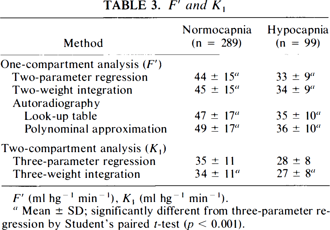
F′ (ml hg⁻¹ min⁻¹), K₁ (ml hg⁻¹ min⁻¹).

Mean ± SD; significantly different from three-parameter regression by Student's paired Mest (p < 0.001).

TABLE 4.

F′/λ and k₂

Method	Normocapnia (n = 289)	Hypocapnia (n = 99)
One-compartment analysis (F′/λ)
Two-parameter regression	0.65 ± 0.15^a	0.55 ± 0.11^a
Two-weight integration	0.67 ± 0.16^a	0.53 ± 0.12^a
Two-compartment analysis (k₂)
Three-parameter regression	0.51 ± 0.14	0.40 ± 0.11
Three-weight integration	0.48 ± 0.15	0.39 ± 0.12

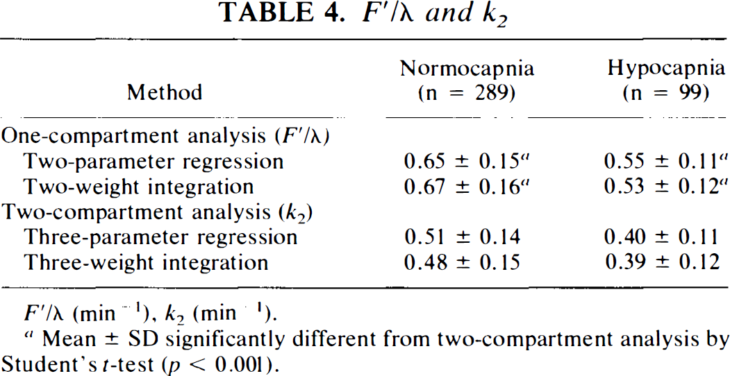
F′/λ (min⁻¹), k₂ (min⁻¹).

Mean ± SD significantly different from two-compartment analysis by Student's t-test (p < 0.001).

K₁ values ± SD determined in four studies without dispersion correction (τ = 0) and using the slope method for tracer delay estimation were 42.10 ± 4.10, 38.38 ± 3.60, 41.50 ± 3.20, and 39.55 ± 5.21 ml hg⁻¹ min⁻¹ while, with dispersion correction (τ = 4 s) and estimation of tracer delay using a global fitting approach (Iida et al., 1989), the corresponding values were 43.43 ± 4.10,39.86 ± 3.93, 41.66 ± 3.20, and 39.34 ± 5.32 ml hg⁻ min⁻¹. As predicted by the simulations, the difference between the two data sets was not statistically significant (p < 0.6).

In the same four studies, V_o values obtained with careful delay and dispersion correction were 1.14 ± 1.18, 0.81 ± 0.71, 1.04 ± 0.93, and 1.22 ± 1.04 ml hg⁻¹, with a global mean of 1.05 ml hg⁻¹, which represents about one-fifty to one-quarter of the average cerebral blood volume (Gjedde, 1988). The large standard deviations were predicted by our simulations (Fig. 2C0.

Hypocapnia caused a reduction of 20–25% for all parameters, regardless of the method of analysis.

Maps

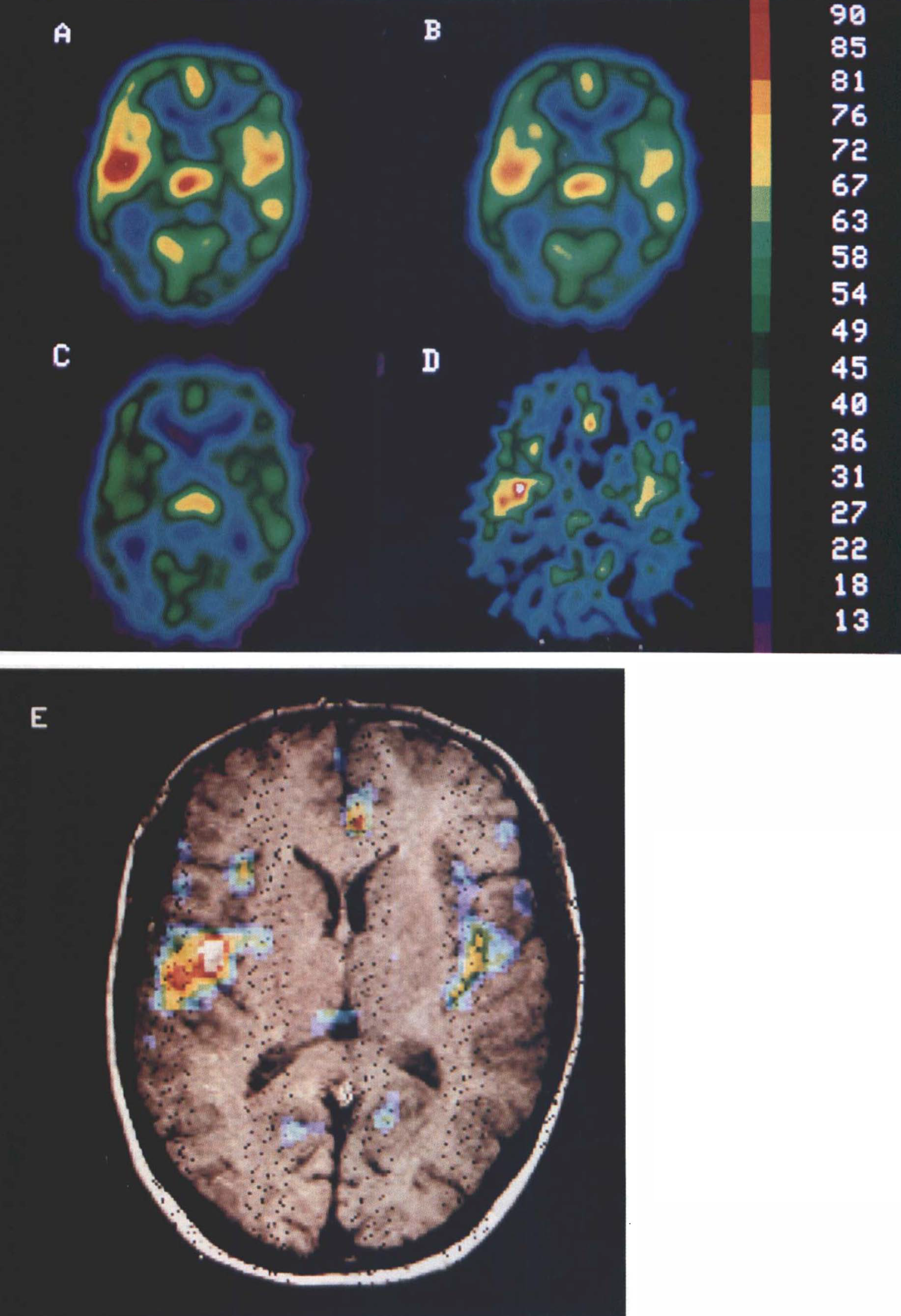
The parameter maps visualize the results obtained, namely that the true water clearance, K₁, is consistently lower than the conventionally derived “blood flow” value, F′, and that this discrepancy is a function, in part, of the apparent vascular distribution, V_o (Figs. 9, 10). The distribution of the V_o maps are consistent with the distribution of known vascular beds. Figures 9 and 10 were derived from a selected water bolus study completed in a single subject using the PC–2048 15B (Scanditronix) tomograph. They enable the comparison of values of F′, K₁, and V_o for various, more or less vascularized, cortical and subcortical brain regions. The two transaxial planes represent (a) an F′ map generated by the look-up table, (b) an F′ map generated by the two-weight integration, (c) a K₁ map generated by the three-weight integration, (d) a V_o map generated by the three-weight integration, and (e) a merger of V_o with the corresponding MR map. The plane shown in Fig. 9 is 6.5 mm above the OM line. The merged maps (Fig. 9E) identify the circle of Willis in the basal cisterna, the middle cerebral arteries in the Sylvian stem, and the posterior cerebral arteries in the ambient cisternae. The F′ maps (Fig. 9A,B) show erroneously high blood flow in the area of the basal cisterna, in which there is no tissue and blood flow, therefore, should be zero. This error does not appear in the K₁ map (Fig. 9C).

FIG. 9.

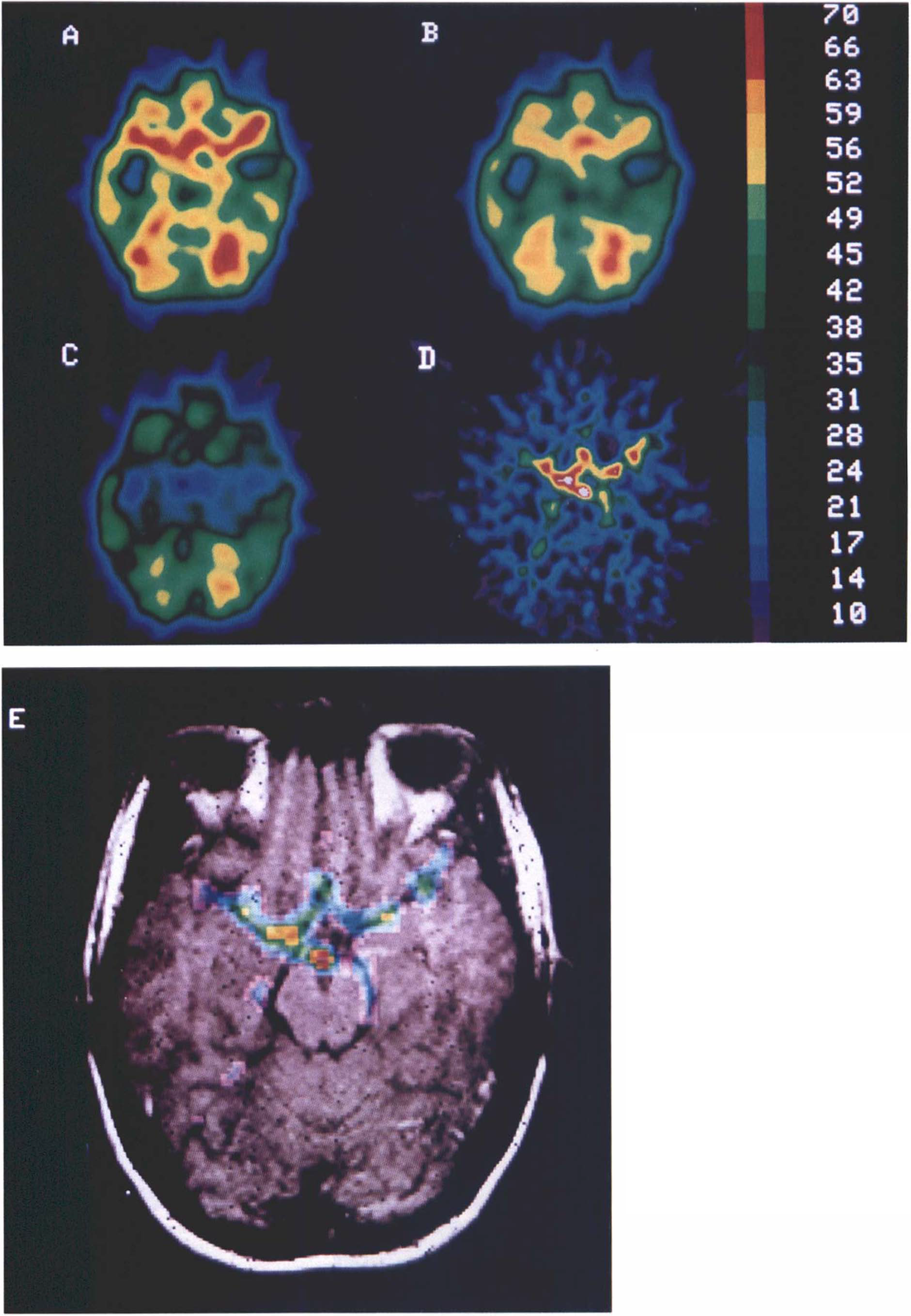
Maps generated from H₂¹⁵O study with the PC–2048 15B tomograph at 6.5 mm above OM line. A: flow (F′) map by look-up table method (λ = 0.9, T = 60 s). B: Flow (F^l) map by two-weight integration (T = 3 min). C: Water clearance (K₁) map, and (D) apparent vascular distribution volume (V_o) map generated by three-weight integration (T = 3 min). E: Merging of V_o and MR maps. Color bar indicates units of F′ and K₁. Maps corresponded to plane 6.5 mm above OM line. Merged maps (E) confirm observation that high intensities of V_o map (D) correspond to circle of Willis in basal cisterna, middle cerebral arteries in Sylvian stem, and posterior cerebral arteries in ambient cisternae. Artefactually high blood flow rates in these regions (maps A, B) are corrected by K₁ map (C).

FIG. 10.

Maps generated from H₂¹⁵O study as in Fig. 9, but 39 mm above OM line. Maps (D) and (E) allow identification of middle cerebral arteries in Sylvian fissures, pericallosal artery in interhemispheric fissure, and medial occipital arteries in parieto-occipital sulci, all sectioned horizontally. Artefactually tifactitiously high blood flow rates in temporal lobes (maps A, B) are corrected in K₁ map (C).

At 39 mm above the OM line (Fig. 10), high intensities are seen (Fig. 10A,B) bilaterally in the insular cisternae (Fig. 10E), which gives the erroneous impression of high blood flow rates in the poles of the temporal lobes and insular gyri. The merged maps (Fig. 10E) demonstrate that the error arises from the middle cerebral arteries in the Sylvian fissure. As evident from the K₁ map (Fig. 10C), the water clearance is no larger in these regions than in other areas of the cortex. The pericallosal artery in the interhemispheric fissure and the medial occipital arteries in the parieto-occipital sulci also are clearly shown in the superposition maps (Fig. 10E) and affect the flow maps (Fig. 10A,B) in the manner just described.

In order to further illustrate the concept of the apparent vascular distribution volume of a tracer, we created three different V_o maps in the plane of the glabellainion line from three studies completed in a single subject using three different tracers (Fig. 11). Figure 11A is a V_o map from a study with H₂¹⁵O, which has a relatively high unidirectional extraction. Figure 11B is a V_o map, obtained as described by Ohta et al., 1992, from a study with [¹⁵O]O₂, which has a relatively low unidirectional extraction. Figure 11C is a V_o map, obtained as described by Ohta et al., 1992 from a study with [C¹⁵]O, which has a negligible unidirectional extraction.

FIG. 11.

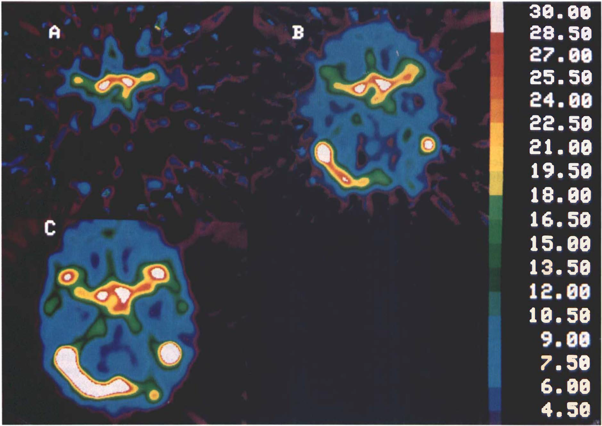
Maps of apparent vascular distribution volume, V_o, obtained at level of glabellainion line from three different studies in same subject. A: V_o map from H₂¹⁵O study. Relatively high unidirectional extraction of water visualizes mainly arterial volume, such as middle cerebral arteries, displayed here. B: V_o map from [¹⁵O]O₂ study. Relatively low unidirectional extraction of oxygen, compared to water, visualizes arterial and partially venous structures. Shown here are transverse sinus and middle cerebral arteries. C: V_o map from [C¹⁵]O study. Since unidirectional extraction of carbon monoxide is negligibly small, map shows entire arterial and venous system. Units of color scale are ml hg⁻¹.

Comparison of the V_o maps supports the following interpretations: The map derived from the [C¹⁵]O study represents the whole blood volume, while the V_o map, calculated from the H₂¹⁵O distribution, represents mainly the arterial volume such as that in the middle cerebral arteries in the Sylvian stem. Finally, the [¹⁵O]O₂-derived V_o map includes part of the venous volume, such as that in the transverse sinus in addition to the middle cerebral arteries, as predicted by Eq. 31.

DISCUSSION

In this report, we show that the single-compartment analysis of brain water uptake significantly overestimates cerebral water clearance. This finding, based on the model proposed here, is not consistent with the claim that flow rates measured with water are too low. Despite this flaw, H₂¹⁵O is widely used for the measurement of CBF by PET. The most common implementations are the single-image continuous inhalation (Frackowiak et al., 1980) and bolus injection (Herscovitch et al., 1983b; Kanno et al., 1987; Raichle et al., 1983) methods. Kinetic (multiframe) methods also have been proposed (Carson et al., 1986), but have not reached the same popularity. Both implementations are based on Kety's single-compartment model (Kety, 1951), which assumes that the tracer is perfectly diffusible, i.e., that there is no diffusion barrier between blood and brain. However, the accuracy of blood flow estimates based on the single-compartment analysis of water uptake has been questioned often, and it has been shown that the diffusion limitation may result in significant underestimation of blood flow (Herscovitch et al., 1987; Raichle et al., 1983). The assumption of an instantaneous equilibrium between blood and brain parenchyma is also an oversimplification, since venous radioactivity concentration is higher than that of brain tissue when complete equilibrium between postarterial blood and tissue is not achieved in a single capillary transit (Koeppe et al., 1987).

Two-compartment and distributed-parameter models have recently been proposed to provide a more adequate description of dynamic blood flow tracer data (Gambhir et al., 1987; Larson et al., 1987; Sawada et al., 1987). These models require at least three parameters, rendering the generation of pixel-by-pixel maps of blood flow from PET data impractical with current algorithms.

In addition to the residual radioactivity in the vascular bed and the limited clearance of the tracer across the capillary endothelium, analysis of water clearance by brain is also affected by the delayed arrival of tracer and its dispersion at the peripheral arterial sampling site. The latter two factors tend to affect estimates of clearance, partition volume, and residual vascular radioactivity, since excess radioactivity in brain may mean either a vascular residuum, early arrival of the bolus, or both. Thus, the corrections for these factors tend to be inversely correlated (Lammertsma et al., 1990).

The present study examines the effect of the delayed equilibration of H₂¹⁵O with brain tissue to answer the question whether reliable clearance rates can be obtained by a one-compartment analysis of cerebral H₂¹⁵O uptake. For this purpose, we studied a two-compartment model consisting of extravascular brain tissue, i.e., brain parenchyma with activity, M_e(t), and a vascular component characterized by the apparent vascular distribution volume, V_o (Evans et al., 1986; Gjedde, 1981; Ohta et al., 1992).

Since a major advantage of PET is its ability to generate functional maps of the brain, visual comparison of images of the same parameter derived from different models provides a qualitative evaluation of the various approaches. Comparison of F′ maps obtained with the one-compartment model (Figs. 9A and 10A, “standard method”) and K₁ maps obtained with the two-compartment model (Figs. 9C and 10C, note that these maps look like blood flow maps, except for a possibly nonlinear scaling function, since K₁ = E₀F for V_c << V_e) revealed striking regional differences, indicating that F′ estimates based on the single-compartment approach must grossly overestimate true water clearance in regions with high, predominantly arterial, vascularity. In some cases, the errors caused by ignoring the vascular radioactivity component were >25%. Other errors, such as tracer arrival delay and dispersion of the arterial input function, tissue heterogeneity and incorrect choice of partition coefficient, were rarely >15%. In other words, the difference between F′ and K₁ cannot be fully eliminated by manipulation of the arterial input function (Iida et al., 1986; Lammertsma et al., 1990).

Compared with K₁ images, the many artifacts in the F′ images are easily recognized, particularly the erroneously high blood flow values in the regions of the major arteries or in the cisternae. As an example, blood flow appeared to be high in the temporal lobes (Fig. 10A,B) due to the proximity of the middle cerebral arteries on the surface of the insular gyrus. This means that the presently accepted values of blood flow for the temporal cortex may be overestimations, since K₁ values appeared not to be higher in the temporal lobe than in other areas of the cortex (Fig. 10C). When compared to corresponding K₁ values, the artificially high conventional F′ values, particularly in highly vascularized regions, indicate that instantaneous equilibrium of H₂¹⁵O between brain tissue and blood is not achieved, contrary to the fundamental assumption underlying the one-compartment model. In other words, blood flow values derived from the one-compartment analysis have limited physiological meaning.

With regard to V_o, which is displayed in Fig. 11 (as derived from studies performed on the same subject with three different tracers, namely H₂¹⁵O, [¹⁵O]O₂, and [C¹⁵]O₂) it is apparent that, as expected, its magnitude decreases as the capillary permeability of the tracer increases (see also Eq. 25). Derived from H₂¹⁵O with its relatively high unidirectional extraction, V_o represents the arterial volume, while when derived from [¹⁵O]O₂ with a relatively low unidirectional extraction, V_o also includes part of the venous volume. Finally, V_o obtained from [C¹⁵]O with its negligible unidirectional extraction reveals the entire arterial and venous circulation. These observations are in line with blood volume estimates derived from ¹⁸F-labeled 2-fluoro-2-deoxy-D-glucose (¹⁸FDG) studies (unidirectional extraction fraction of ∼0.2) by Evans et al. (1986).

Values of blood volume and V_o can be read from Fig. 11, noting that V_o, unlike K₁, is very sensitive to dispersion of the tracer in the radial artery and errors in the time delay determination (Fig. 4A,B). For the generation of K₁ and V_o maps, dispersion in the radial artery is accounted for in a subsequent article, rather than in the present. For K₁ estimates, the consequent error was <5% for a typical dispersion time constant of τ = 4 s (Fig. 3A). On the other hand, V_o is so sensitive to image noise (Fig. 2C) as well as to the effects of dispersion and tracer arrival delay (Fig. 4) that its exact magnitude is highly uncertain. In particular, ignoring dispersion always results in an overestimation of V_o. Our attempt to quantify V_o in four cases in which dispersion and tracer arrival delay had been carefully corrected yielded an average of V_o = 1.05 ml hg⁻¹, which amounts to 22% of an accepted literature value for the entire average cerebral blood volume of 4.8 ml hg⁻¹ (Gjedde, 1988). This result is consistent with Eq. 25 and our observation (Figs. 9 –11) that V_o derived from H₂¹⁵O is weighted towards the arterial component of the cerebral vascular volume. When mapped on a pixel-by-pixel basis, V_o estimates accurately outline major vessels in many areas (Fujita et al., 1996). We regard this as sufficient assurance that two compartments are more appropriate than one compartment for providing accurate estimations of CBF.

Our measurements on human subjects, analyzed with a more realistic two-compartment model of transport and clearance at the capillary endothelium, suggest that the widely used one-compartment model systematically overestimates local CBF. We note that, even when an infinitely diffusible tracer is used, a correction for the vascular component may, therefore, be necessary to account for tracer not exchanged in the arterial vasculature under physiological conditions.

Footnotes

Acknowledgment:

This work was supported by MRC (Canada) grants PG-41 and SP-30, the Isaac Walton Killam Fellowship Fund of the Montreal Neurological Institute, and by the Quebec Heart Foundation. We thank the technical staff of the McConnell Brain Imaging Centre, and the Neurophotography Department for their assistance. Special thanks are due Mr. Peter Neelin for providing the registered MR images. The helpful comments of Dr. Hiroto Kuwabara as well as the contribution of Professor Ludvik Bass, Department of Biomathematics, University of Brisbane, Brisbane, Australia, are particularly appreciated.

APPENDIX

Two-compartment analysis. Capillary permeability. Assume that local microvascular properties (F, P_dA, V_d) are uniform within a brain ROI in which P_d is the apparent permeability of the endothelium to a tracer passing from the blood to the tissue, A is the capillary surface area, F is the blood flow, V_c is the volume of the capillary bed, C_c is the concentration of the tracer in this volume, V_d is the volume of the extravascular space, C_e is the uniform tracer concentration in this space, α₁ is the solubility coefficient of the capillary fluid, and α₂ is the solubility coefficient of the extravascular fluid. Initially, we assume that the region includes no arterial or venous volume. Below, these will be added to the region (see Arterial and venous volumes). The compartmental assumption that C_e is uniform means that the incremental addition made to C_e during a single passage of a single capillary is negligible. It also means that discontinuities must exist at both ends of the capillary bed, such that the concentration is C_a at the single inlet and, on the average, C̅_c in the capillary bed between the single inlet and single outlet. Also, it is assumed that brain capillaries do not run in parallel; rather, they are believed to form intricate convolutions that contribute to the uniformity of C_e.

The solubility coefficients are defined as the ratios α₁ ≡ V_c/V^ω_c and α₂ ≡ V_d/V^ω_d where V_c^ω and V_d^ω are defined as the water volumes of V_c and V_d, respectively. Assuming uniform concentration within an elemental capillary crossection, tracer transport across the entire wall of the capillary bed is then described by the equation

(9)

V_{d} \frac{d C_{e}}{dt} = p_{d} A (\frac{C_{c}}{α_{1}} - \frac{C_{e}}{α_{2}})

Derivation of M_c. The symbol M_c represents the quantity of tracer in the capillary bed, equal to the product of V_c and C̅_c. To determine C̅_c, let C_c(τ) be the capillary tracer concentration in a small volume of plasma, ΔV_c, at the time τ after its entry into a capillary

(10)

Δ V_{c} \frac{d C_{c} (τ)}{d τ} = p_{d} Δ A \frac{M_{e}}{V_{d}} - P_{d} Δ A \frac{C_{c} (τ)}{α_{1}}

where M_e is the tracer product V_dC_e, which is not assumed to change appreciably during a single capillary transit. The average of all transit times, , equals V_c/F. As ΔA/ΔV_c = A/V_c and C_c(0) = C_a, integration from τ = 0 to τ = u for any single transit yields

(11)

C_{c} (u) = C_{a} e^{- P \cdot u / [F \cdot \bar{τ}]} + \frac{M_{e}}{V_{e}} (1 - e^{- P \cdot u / [F \cdot \bar{τ}]})

Here, we define P = P_dA/α₁ and V_e = V_d/α₁. The term V_e represents the tissue distribution volume, corrected for any difference between the solubility coefficients of the capillary bed and the brain tissue proper. The capillary bed can now be simulated by a single imaginary vessel with a volume of V_c, surface area A, and flow of F, with sufficient cross-sectional involutions to render cross-sectional gradients nonexistent. The mean tracer concentration in this vessel is then the average of all concentrations of this capillary

(12)

\begin{array}{l} {\bar{C}}_{c} & = & \frac{1}{τ} \int_{o}^{τ} C_{c} (u) du \\ = & \frac{F}{P} (1 - e^{- P / F}) C_{a} + \frac{M_{e}}{V_{e}} [1 - \frac{F}{P} (1 - e^{- P / F})] \end{array}

where 1 — e^−P/F is revealed as the extraction fraction, E_o, for unidirectional transfer of tracer into the tissue (Crone, 1963), i.e., for M_e = 0

(13)

E_{o} \equiv 1 - e^{- P / F} = \frac{P {\bar{C}}_{c}}{F C_{a}}

The concentration C̅_c varies both with C_a and with the tissue concentration of tracer, which, in turn varies with C_a. Generally speaking, therefore, C̅_c is lowest initially when C_e ∼ 0 and highest at the steady-state level C_a.

The quantity of tracer in the capillary bed is calculated from Eqs. 12 and 13

(14)

M_{c} = V_{c} {\bar{C}}_{c} = V_{o} C_{a} + (V_{c} - V_{o}) \frac{M_{e}}{V_{e}}

where V_o is the apparent vascular volume of distribution. Since we have not yet introduced arterial and venous volumes, V_o is temporarily defined as the portion of the true vascular volume of distribution, V_c, that equals the quotient V_cE_oF/P. Below, V_o and V will be expanded with arterial and venous volumes. Equation 11 indicates that the capillary tracer content, M_c, changes as a function of M_e. This result shows that the tracer in the capillary bed has two apparent states, one at the arterial concentration in the volume V_o, and one at the tissue concentration (corrected for a difference in solubility) in the remaining volume of the capillary bed.

Derivation of M_e. The net transport of tracer across the endothelium is given by Eqs. 9 and 12

(15)

\frac{d M_{e}}{dt} = F (1 - e^{- P / F}) C_{a} F (1 - e^{- P / F}) \frac{M_{e}}{V_{e}}

in which M_e is the product V_d × C_e. When k₂ is the rate constant of tracer washout from the compartment M_e

(16)

k_{2} \equiv F (1 - e^{- P / F}) / V_{e} = E_{o} F / V_{e}

Eq. 15 reduces to

(17)

\frac{d M_{e}}{dt} = k_{2} V_{e} C_{a} - k_{2} M_{e}

The solution to Eq. 17 is

(18)

M_{e} = k_{2} V_{e} \int_{o}^{T} C_{a} e^{- k_{2} (T - t)} dt

Derivation of M. For a two-compartment system (Fig. 1, left panel), having the two compartments M_c and M_e, according to Eq. 14, the total amount of tracer in the RO1 is

(19)

M = M_{c} + M_{e} = V_{o} C_{a} + (V - V_{o}) \frac{M_{e}}{V_{e}}

where V ≡ V_c + V_e.

Inserting Eq. 18 into Eq. 19, we obtain the total tracer quantity in the tissue

(20)

M = V_{o} C_{a} + K_{1} \int_{o}^{T} C_{a} e^{- k_{2} (T - t)} dt

where K₁, the water blood-brain clearance, is defined by the relationship

(21)

K_{1} \equiv k_{2} (V - V_{o})

The term clearance is adopted from kidney physiology where it refers to the removal of substances from the circulation. Equations 20 is the solution to the equation

(22)

\frac{dM}{dt} = V_{o} \frac{d C_{a}}{dt} + (K_{1} + k_{2} V_{o}) C_{a} - k_{2} M

From the definition of V_o, it follows that V_o approaches the capillary volume V_c and V — V_o the partition volume V_e, only for low values of P relative to E_oF. For large values of P, V_o includes no fraction of the capillary vascular bed (V_o approaches V_a, see below for explanation), and V — V_o approaches V_e + V_c.

By integration of Eq. 22, we obtain the integral solution

(23)

M = V_{o} C_{a} + (K_{1} + k_{2} V_{o}) \int_{o}^{T} C_{a} dt - k_{2} \int_{o}^{T} M dt

Arterial and venous volumes. The above derivation was based on tissue with exchange vessels and extravascular tissue, i.e., tissue without appreciable arterial or venous components. For tissue that also includes arteries and arterioles, and venules, and veins, represented by the volume V_a and V_v, respectively, the terms V and V_o in Eq. 19, 21, and 23 must be expanded as follows:

(24)

V = V_{a} + V_{c} + V_{e} + V_{v}

and

(25)

V_{o} = V_{a} + V_{c} \frac{E_{o} F}{P} + V_{v} (1 - E_{o})

Thus, when P is large relative to F, E_o approaches unity and V_o reduces to V_a.

One-compartment analysis. When H₂¹⁵O is used to measure CBF by a one-compartment analysis, the tacit assumption is made that H₂¹⁵O is inert and perfectly diffusible, i.e., faces no diffusion barriers between the vascular space and brain tissue, and that tracer delivery to the brain is only limited by the blood flow, F (Fig. 1, right panel). Thus, in the conventional one-compartment approach, the tracer in brain tissue, including its vascular bed, occupies a single compartment. This model ignores the result of the above derivation, which indicates that V_o is at least equal to V_a. Hence, we must evaluate the assumption of zero V_o as if it were appropriate for a tracer of infinitely high permeability. When P >> F, E_o approaches unity, and V_o declines to V_a. These changes cause Eq. 22 to reduce to

(26)

\frac{d M (t)}{dt} = V_{a} \frac{d C_{a} (t)}{dt} + \frac{F}{V_{e}} V C_{a} (t) - \frac{F}{V_{e}} M (t)

To obtain the commonly used form, we must assume that V_a is zero

(27)

\frac{d M (t)}{dt} = F^{'} C_{a} (t) - \frac{F^{'}}{λ} M (t)

where F′ equals FV/V_e and equals V. F′ is the resulting estimate of “blood flow” and λ is the corresponding estimate of the volume V. Therefore, F′ equals the parameter F and λ equals the parameter V_e, only when the vascular volumes V_a + V_c + V_v are negligible compared to V_e.

Abbreviations used

References

Alpert

Eriksson

Chang

Bergström

Litton

Correia

Bohm

Ackerman

Taveras

(1984) Strategy for the measurement of regional cerebral blood flow using short-lived tracers and emission tomography. J Cereb Blood Flow Metab 4:28–34

Carson

Huang

Green

(1986) Weighted integration method for local cerebral blood flow measurements with positron emission tomography. J Cereb Blood Flow Metab 6:245–258

Cooke

Evans

Fanthome

Alarie

Sendyk

(1984) Performance figures and images from the Therascan 3128 positron emission tomograph. IEEE Trans Nucl Sci NS-31: 640–644

Crone

(1963) The permeability of capillaries in various organs as determined by use of the ‘indicator diffusion’ method. Acta Physiol Scand 58:292–305

Eichung

Raichle

Grubb

Ter-Pogossian

(1974) Evidence of the limitation of water as a freely diffusible tracer in brain of the rhesus monkey. Circ Res 35:358–364

Evans

Diksic

Yamamoto

Kato

Dagher

Redies

Hakim

(1986) Effect of vascular activity in the determination of rate constants for the uptake of 15F-labeled 2-fluoro-2-deoxy-D-glucose: Error analysis and normal values in older subjects. J Cereb Blood Flow Metab 6:724–738

Evans

Marrett

Collins

Peters

(1989) Anatomical-functional correlative analysis of the human brain using three dimensional imaging systems. Proc SPIE 1092:264–274

Evans

Thompson

Marrett

Meyer

Mazza

(1991) Performance evaluation of the PC–2048: A new 15-slice en-coded-crystal PET scanner for neurological studies. IEEE Trans Med Imaging 10:90–98

Frackowiak

RSJ

Lenzi

Jones

Heather

(1980) Quantitative measurement of regional cerebral blood flow and oxygen metabolism in man using 15O and positron emission tomography: Theory, procedure, and normal value. J Corn-put Assist Tomogr 4:727–736

10.

Fujita

Kuwabara

Meyer

Gjedde

(1992) Intravascular radioactivity in brain affects estimates of the arrival delay of [0–15] tracers [abstract]. J Nude Med 33:909

11.

Fujita

Meyer

Reutens

Kuwabara

Evans

Gjedde

(1996) Cerebral [15O] water clearance in humans determined by PET: II. Vascular responses to vibrotactile stimulation. J Cereb Blood Flow Metab 16 (in press)

12.

Gambhir

Huang

Randall

Phelps

(1987) A study of the single compartment tracer kinetic model for the measurement of local cerebral blood flow using 15O-water and positron emission tomography. J Cereb Blood Flow Metab 7:13–20

13.

Gjedde

Andersson

Eklöf

(1975) Brain uptake of lactate, antipyrine, water and ethanol. Acta Physiol Scand 93:145–149

14.

Gjedde

(1981) High- and low-affinity transport of D-glucose from blood to brain. J Neurochem 36:1,463–1,471

15.

Gjedde

(1988) Concluding remarks: In: Cerebral Hyperemia and Ischemia: From the Standpoint of Cerebral Blood Volume ( Tomita

Sawada

Naritomi

Heiss

W-D

, eds), Amsterdam, New York, Oxford, Elsevier Science Publishers BV (Biomedical Division), Excerpta Medica, pp 277–280

16.

Grubb

Raichle

Higgins

Eichung

(1978) Measurement of regional cerebral blood volume by emission tomography. Ann Neurol 4:322–328

17.

Herscovitch

Mintun

Raichle

(1983a) Effect of tissue heterogeneity on the measurement of cerebral blood flow with the equilibrium [C15]O2 inhalation technique. J Cereb Blood Flow Metab 3:407–415

18.

Herscovitch

Mintun

Raichle

(1983b) Brain blood flow measured with intravenous H215O. 1. Theory and error analysis. J Nude Med 24:782–789

19.

Herscovitch

Raichle

Kilbourn

Welch

(1987) Positron emission tomographic measurement of cerebral blood flow and permeability-surface area product of water using [15]O water and [11C] butanol. J Cereb Blood Flow Metab 7:527–542

20.

Iida

Kanno

Miura

Murakami

Takahashi

Uemura

(1986) Error analysis of a quantitative cerebral blood flow measurement using 0–15 H2O autoradiography and positron emission tomography, with respect to the dispersion of the input function. J Cereb Blood Flow Metab 6:536–545

21.

Iida

Kanno

Miura

Murakami

Takahashi

Uemura

(1989) A determination of the regional brain/blood partition coefficient of water using dynamic positron emission tomography. J Cereb Blood Flow Metab 9:874–885

22.

Kanno

Iida

Miura

Murakami

Takahashi

Sasaki

Inugami

Shishido

Uemura

(1987) A system for cerebral blood flow measurement using an H215O autoradiographic method and positron emission tomography. J Cereb Blood Flow Metab 7:143–153

23.

Kety

(1951) Theory and applications of exchange of inert gas at lungs and tissue. Pharmacol Rev 3:1–41

24.

Koeppe

Holden

(1985) Performance comparison of parameter estimation techniques for the quantitation of local cerebral blood flow by dynamic positron computed tomography. J Cereb Blood Flow Metab 5:224–234

25.

Koeppe

Hutchins

Rothley

Hichwa

(1987) Examination of assumptions for local cerebral blood flow studies in PET. J Nucl Med 28:1,695–1,703

26.

Lammertsma

Cunningham

Deiber

Heather

Bloomfield

Nutt

Frackowiak

RSJ

Jones

(1990) Combination of dynamic and integral method for generating reproducible functional CBF images. J Cereb Blood Flow Metab 10:675–686

27.

Larson

Markham

Raichle

(1987) Tracer-kinetic models for measuring cerebral blood flow using externally detected radiotracers. J Cereb Blood Flow Metab 7:443–463

28.

Lassen

(1985) Normal average value of cerebral blood flow in younger adults is 50 ml/100 g/min [Editorial]. J Cereb Blood Flow Metab 5:347–349

29.

Meyer

Tyler

Thompson

Redies

Diksic

Hakim

(1987) Estimation of cerebral oxygen utilization rate by single bolus 15O2 inhalation and dynamic positron emission tomography. J Cereb Blood Flow Metab 7:403–414

30.

Meyer

(1989) Simultaneous correction for tracer arrival delay and dispersion in CBF measurements by the H215O autoradiographic method and dynamic PET. J Nucl Med 30:1,069–1,078

31.

Ohta

Meyer

Thompson

Gjedde

(1992) Oxygen consumption of the living human brain measured after a single inhalation of positron emitting oxygen. J Cereb Blood Flow Metab 12:179–192

32.

Raichle

Martin

WRW

Herscovitch

Mintun

Markham

(1983) Brain blood flow measured with intravenous H215O 11. Implementation and validation. J Nucl Med 24:790–798

33.

Sawada

Sugiyama

Iga

Hanano

(1987) Tracer disposition kinetics in the determination of local cerebral blood flow by a venous equilibrium model, tube model, and distributed model. J Cereb Blood Flow Metab 7:433–442

34.

Thompson

Dagher

Meyer

Evans

(1986) Imaging performance of a dynamic positron emission tomograph: Positome IIIp. IEEE Trans Med Imaging 5:183–198

Cerebral [ 15 O]Water Clearance in Humans Determined by PET: I. Theory and Normal Values

Abstract

Keywords

EXPERIMENTAL DESIGN AND THEORY

METHODS

Simulated PET studies

Human studies

Data analysis

RESULTS

Simulated PET studies

Human studies

Maps

DISCUSSION

Footnotes

Acknowledgment:

APPENDIX

Abbreviations used

References