
Abstract
Continuous arterial spin labeling (CASL) magnetic resonance imaging (MRI) was combined with multivariate analysis for detection of an Alzheimer's disease (AD)-related cerebral blood flow (CBF) covariance pattern. Whole-brain resting CBF maps were obtained using spin echo, echo planar imaging (SE-EPI) CASL in patients with mild AD (n=12, age=70.7±8.7 years, 7 males, modified Mini-Mental State Examination (mMMS)=38.7/57±11.1) and age-matched healthy controls (HC) (n=20; age=72.1±6.5 years, 8 males). A covariance pattern for which the mean expression was significantly higher (P<0.0005) in AD than in HC was identified containing posterior cingulate, superior temporal, parahippocampal, and fusiform gyri, as well as thalamus, insula, and hippocampus. The results from this analysis were supplemented with those from the more standard, region of interest (ROI) and voxelwise, univariate techniques. All ROIs (17/hemisphere) showed significant decrease in CBF in AD (P<0.001 for all ROIs, αcorrected=0.05). The area under the ROC curve for discriminating AD versus HC was 0.97 and 0.94 for covariance pattern and gray matter ROI, respectively. Fewer areas of depressed CBF in AD were detected using voxelwise analysis (corrected, P<0.05). These areas were superior temporal, cingulate, middle temporal, fusiform gyri, as well as inferior parietal lobule and precuneus. When tested on extensive split-half analysis to map out the replicability of both multivariate and univariate approaches, the expression of the pattern from multivariate analysis was superior to that of the univariate.
Introduction
Cerebral blood flow (CBF) is commonly accepted as a physiologic correlate of normal brain metabolism and a biomarker of several brain pathologies (Gonzalez et al, 1995). Perfusion imaging techniques such as H2O15 positron emission tomography (PET), single-photon emission computed tomography (SPECT), dynamic contrast enhanced magnetic resonance imaging (DCE MRI), and arterial spin labeling (ASL) MRI have proven to be indispensable tools in studying brain pathologies such as Alzheimer's disease (AD) (Alsop et al, 2000; Du et al, 2006; Herholz et al, 2002; Johnson et al, 1998; Scarmeas et al, 2004; Silverman et al, 2001). Most AD imaging studies have relied on PET and SPECT and have shown a marked decrease in metabolism and/or regional blood flow in the AD population (Herholz et al, 2002; Johnson et al, 1998; Scarmeas et al, 2004; Silverman et al, 2001). Results from several ASL studies have shown good agreement across techniques (Alsop et al, 2000; Du et al, 2006; Johnson et al, 2005; Sandson et al, 1996). Regardless of the particular imaging technique employed, the general conclusion from these studies is that a quantitative measurement of CBF has the potential of being the imperative biomarker for early detection and diagnosis of AD.
Arterial spin labeling offers several practical and scientific advantages over the other techniques: (1) it is amenable to safe and economical repeated measurements, because it uses arterial blood water as an endogenous tracer, thus avoiding the need for injection of expensive and potentially harmful tracers required in PET, SPECT, or DCE MRI; (2) it provides CBF quantification without arterial blood sampling, which can be extremely uncomfortable for subjects but necessary for quantitative PET; (3) it can be acquired in the same session with structural and other MR images; and (4) ASL CBF measurements are stable across sessions, making this technique ideal for tracking CBF changes over time due to recovery or therapeutic intervention (Floyd et al, 2003; Parkes et al, 2004).
Arterial spin labeling techniques have been used in a variety of applications in both disease and normal brain function (Alsop and Detre, 1998; Golay et al, 2004). On the basis of differences in the way the arterial water is labeled, ASL methods are generally classified as continuous ASL (CASL) or pulsed ASL (PASL). Compared with PASL, CASL has been shown to have higher signal-to-noise ratio (SNR) and offers whole-brain coverage via multislice acquisition (Wang et al, 2002).
Arterial spin labeling has already been used in studies of AD (Alsop et al, 2000; Du et al, 2006; Johnson et al, 2005; Sandson et al, 1996). The importance of these studies has been twofold. First, they have served as validation of ASL in studying AD by showing good agreement with hexamethylpropyleneamine (HMPAO) SPECT (El Fakhri et al, 2004; Johnson et al, 1998). Second, the overlap in regions of hypoperfusion obtained with ASL with those of decreased metabolism detected with fluorodeoxyglucose PET supports the hypothesis of a direct coupling between these two effects in AD (Herholz et al, 2002).
Only one of the aforementioned ASL studies used CASL (Alsop et al, 2000) and found areas of significant CBF depression in temporal, parietal, frontal, and posterior cingulate cortices in the AD group as compared to healthy controls (HC). The other three studies have reported data from PASL, which, in addition to lower SNR, has the disadvantage of being restricted only to a slab commonly placed in the superior cerebral cortex, thus excluding major portions of the temporal and inferior frontal lobes (Du et al, 2006; Johnson et al, 2005; Sandson et al, 1996). Furthermore, a nonquantitative version of PASL was used and therefore only relative measurements (in percent change) of CBF were reported. In all these studies, univariate statistical analysis was employed for the between-group comparisons.
One of the goals of this paper is to show the feasibility of combining CASL with multivariate analysis for detection of an AD-related CBF covariance pattern that contrasts AD patients and HC at baseline. Multivariate approaches evaluate correlation/covariance of CBF measurement across brain regions rather than proceeding on a region-by-region (or voxel by voxel) basis. Thus, their results can be more easily interpreted as a functional signature of neural networks (Habeck et al, 2005).
However, owing to higher computational and conceptual complexity as well as the absence of an easy-to-use software package, multivariate techniques have rarely been applied in clinical imaging.
A study by Scarmeas et al (2004) applied covariance analysis to nonquantitative H2O15 PET data and found a pattern whose mean expression was higher in AD than in controls. When prospectively applied to a sample of minimally to mildly cognitively impaired subjects, the expression of the AD-related pattern was predictive of cognitive performance at baseline as well as of the subsequent decline; subjects who had higher baseline expression of the AD-related pattern showed lower cognitive performance and declined faster (Scarmeas et al, 2004).
Our study is the first to combine multivariate analysis with CASL imaging to investigate its utility for differential diagnosis of AD. Furthermore, we compare the sensitivity of diagnosis of the multivariate technique with that obtained using the more standard ROI- or voxel-based univariate analyses.
Methods
Subjects
Resting CBF maps were obtained using CASL images from 12 subjects (age 70.7±8.7 years, 7 males) diagnosed with mild AD using NINCDS-ADRDA (National Institute of Neurological and Communicative Diseases and Stroke/Alzheimer's Disease and Related Disorders Association) criteria (McKhann et al, 1984) and 20 age-matched HC (age 72.4±6.5 years, 8 males).
Alzheimer's disease and HC subjects were recruited from outpatients who were presented to the Alzheimer's Disease Research Center at Columbia University. Alzheimer's disease patients met Diagnostic and Statistical Manual of Mental Disorders-Version 3-Revised (DSM-III-R) criteria for dementia and NINCDS-ADRDA criteria for probable AD (McKhann et al, 1984) and underwent a thorough diagnostic evaluation including neurologic examination, neuropsychological testing, functional evaluation, and rating of basic and instrumental activities of daily living (Benton and Hamsher, 1976; Buschke and Fuld, 1974; Stern et al, 1987; Wechsler, 2001). Other causes of dementia were excluded with appropriate laboratory tests. On the basis of a comprehensive review of all available information, a consensus diagnostic conference of neurologists, psychiatrists, and neuropsychologists determined the diagnosis of AD and finalized a Clinical Dementia Rating (CDR) (Hughes et al, 1982). Only AD patients rated as CDR=1 were used in this study. CASL MRI results did not play any role in the diagnostic process.
Potential healthy elderly controls were recruited from family members and advertisement. They were carefully screened with medical, neurologic, psychiatric, and neuropsychological evaluations to exclude those with dementia or cognitive impairment (Nelson and O'Connell, 1978; Stern et al, 1987; Wechsler, 1981, 2001), as well as other neurologic, psychiatric, or severe medical disorders. Subjects with space occupying lesions or vascular disease were excluded. White matter (WM) hyperintensities were permitted, but any clinical evidence (symptoms or signs) of stroke or MRI evidence of cortical or lacunar infarcts constituted exclusion criteria.
All subjects received the modified Mini-Mental State Examination (mMMS) as a global rating of cognitive function. This is a 57-point modification of the original MMSE (Folstein et al, 1975) that includes the addition of digit span forward and backward (Wechsler, 1981) two additional calculation items, recall of the current and four previous presidents of the country, confrontation naming of 10 items from the Boston Naming Test (Kaplan et al, 1983), one additional sentence to repeat, and a different copy task including two figures.
All subjects provided written consent as approved by the Columbia University Medical Center Institutional Review Board.
Magnetic Resonance Imaging Acquisition
Spin echo, echo planar imaging CASL images were acquired on a 1.5 T Philips Intera scanner using the manufacturer's head transmit—receive coil with labeling duration=2,000 ms, postlabeling delay (PLD)=800 ms, echo time/repetition time (TE/TR)=35 ms/5,000 ms, flip angle=90°, acquisition matrix 64 × 58, field of view=220 mm2 × 193 mm, slice thickness=7.5 mm/1.5 mm gap, number of transaxial slices=15. Slices were acquired in ascending mode (i.e., inferior to superior) with a slice acquisition time of 64 ms. Total number of CBF images per subject was 30.
To check for the effect of transit time in the CBF measurement, in six AD patients, two sets of CASL CBF images were acquired: one with a moderate PLD of 0.8 secs and another with a longer PLD of 1.0 secs.
To induce the flow-driven adiabatic inversion (labeling) of the water spins, a ‘block-shaped’ radio frequency (RF) pulse 2,000 ms long and 35 mG amplitude in the presence of a z-gradient 0.25 G/cm was applied before acquisition of each labeled image (Alsop and Detre, 1996). To correct for off-resonance saturation effects, an amplitude-modulated (sinusoidal, 250 Hz) RF pulse of the same power and gradient was applied before the acquisition of each control image (Alsop and Detre, 1996). The frequency offset of the RF pulses was set to position the labeling plane 40 mm inferior to the lower edge of the imaging volume.
To spatially normalize images into standard space, a high-resolution, T1-weighted, three-dimensional spoiled gradient image (SPGR) was acquired in each subject with TE/TR=3 ms/34 ms, flip angle=45°, acquisition matrix=256 × 256 × 124, voxel size=0.94 × 0.94 × 1.29 mm3.
The scanning session started with the rapid (35 secs) acquisition of a T1-weighted image to determine patient position. Subjects were instructed to relax and minimize motion during the scan. Foam padding was inserted around the sides of the head and the forehead to minimize patient motion.
Magnetic Resonance Imaging Data Preprocessing
All image preprocessing was implemented using SPM99 software (Wellcome Department of Cognitive Neurology) and code written in MATLAB (Mathworks, Natick, MA, USA). For each subject, images were preprocessed as follows: (i) all control and labeled EPI images were realigned to the first acquired using SPM's automated realignment algorithm. (ii) The T1-weighted structural image and the first acquired EPI image were coregistered using the mutual information coregistration algorithm in SPM99. (iii) The structural image was then used to determine parameters (7 × 8 × 7 nonlinear basis functions) for transformation into Talairach standard space defined by the Montreal Neurologic Institute (MNI) template brain supplied with SPM99. (iv) This transformation was then applied to all the EPI images, which were re-sliced using sinc interpolation to 2 mm × 2 mm × 2 mm. (v) SPM99 was used to segment the structural images into gray matter (GM), WM, and cerebrospinal fluid posterior probability maps were needed for masking and computation of CBF.
Computation of Cerebral Blood Flow
The spatially normalized control/label pairs were used to calculate percent change maps, which were subsequently used to compute CBF using the two-compartment formula derived by Alsop and Detre (1996) and later modified by Wang et al (2002). The following parameter values were used: longitudinal relaxation, (T1) of blood=1,400 ms; blood/tissue water partition=0.9 mL/g; transit time=1,300 ms; labeling duration=2,000 ms; tissue T1 in absence of RF=1,150 and 800 ms for GM and WM, respectively; T1 in presence of RF=750 and 530 ms for GM and WM, respectively (Alsop and Detre, 1996); PLD adjusted to account for the slice acquisition time, PLDs=(acquisition slice−1) × (64 ms)+800 ms; labeling efficiency for CASL at 1.5 T on Philips Intera is 0.70 (Werner et al, 2005).
For each subject, GM, WM, and cerebrospinal fluid posterior probability images were obtained using SPM99 and subject's SPGR. For each voxel, computation of CBF was weighted by the tissue-type posterior probability.
To get rid of any signal from scalp and nonbrain tissue, a mask including only voxels with an SE-EPI intensity >0.80 was obtained and used to yield an average CBF image for each subject before any statistical analysis.
For the voxelwise analysis (in both multi- and univariate versions), CBF images were spatially smoothed with a 6 mm kernel. No smoothing was carried out for the ROI analysis.
Covariance Analysis
To identify CBF network correlates of early dementia, we employed an analysis technique that originated from the Scaled Subprofile Model, a covariance analysis method (Moeller et al, 1987) that has been used previously in resting imaging studies of normal aging and a variety of neurologic diseases (Hutchinson et al, 2000; Moeller et al, 1999; Nakamura et al, 2001). We summarize the steps of this algorithm in detail; no room has been left for arbitrary decisions on the part of the analyst:
Zero-meaned average CASL CBF images from all subjects from both groups were simultaneously included in a single principal component (PC) analysis, which captures the major sources of between- and within-groups variation, producing a series of PCs. Voxels participating in each PC may have either a positive or a negative loading. Voxels with positive loadings can be conceived as exhibiting concomitant increased flow and those with negative loadings can be conceived as exhibiting concomitant decreased flow.
The expression of each PC for each subject was quantified by a subject scaling factor (SSF). A higher SSF value indicates more prominent concomitantly increased flow of the voxels with positive loadings and more prominent concomitantly decreased flow of the voxels with negative loadings. In other words, the SSF expresses the degree of subject's expression of the fixed PC.
To identify a covariance pattern that best discriminates AD patients from controls, each subject's SSFs of the specified PCs derived from step 1 together with a spatially uniform image representing the average CBF (since absolute quantification is provided with CASL) was entered into a linear regression model as the independent variable. Group membership (AD versus HC) was the dependent variable. This regression resulted in a linear combination of the first PCs and the uniform image that best discriminated the two groups. This linear combination of the PCs can itself be conceived of as signifying a ‘pattern’ or ‘network.’ The area under the Receiver Operator Characteristic (ROC) curve (AUC) was used to determine how many PCs out of the first six should be included in the regression. The four PCs and the spatially uniform average CBF image were included in the analysis, as they achieved the largest AUC value of 0.96.
Estimation of Robustness of Regional Weights in Covariance Pattern
Continuous arterial spin labeling CBF patterns resulting from multivariate analysis assign different weights to all voxels included in the analysis, depending on the salience of their covariance contribution. Positive voxel weights indicate a positive correlation between the subject's expression value and the associated regional ASL signal; negative weights indicate a negative correlation. This means that as the expression of a pattern increases, ASL signal in the positively weighted regions increases as well, whereas ASL signal in the negatively weighted regions decreases. The absolute magnitude of a regional weight determines the slope of this change; for instance, a region whose weight is twice as large as that of another also changes its ASL signal twice as steeply. Whether a voxel weight is reliably different from zero is assessed by a bootstrap estimation procedure (Efron and Tibshirani, 1994). This entails repeating the derivation of the covariance patterns (regardless of whether cross-sectional or longitudinal) many times on the resampled subject data to approximate the variability of the regional weights with their s.d. incurred through the resampling process. Denoting the point estimate of a voxel weight as w, and the s.d. resulting from the bootstrap-resampling procedure as s w , we can calculate a rough z-statistic according to z=w/s w . Sufficiently small variability of a voxel weight around its point estimate results in a large magnitude of z and indicates a reliable contribution to the covariance pattern. Under the assumptions of a standard-normal distribution for z, z∼N(0,1), choosing a threshold of ∣z∣>3.09 results in a one-tailed P-level that is smaller than 0.001.
Nonparametric Test of the Null Hypothesis Using the Method of Permutations
To avoid having to rely on parametric distribution 4 theory and its associated simplifying assumptions, we performed a permutation test. We resampled the data from both groups, HC and AD, and recomputed the complete analysis stream for 10,000 iterations, each time breaking the group-subject assignment, while keeping the group strengths, 12 and 20, the same. The Principal Component Analysis (PCA) step is invariant 4with respe4 ct to this resampling operation, but the discriminant analysis will give different results. We computed the null-4 hypothesis histogram, using the t-statistic derived from the pattern expressions in both groups. The P-level is read off as the fraction of permutations that gave rise to a bigger value of the test statistic than the point estimate. We performed this test on both the group-contrast t-value and AUC of the AD-pattern expression.
To check for the presence of a gender effect, a two-tailed t-test was run between SSF scores and gender across both groups and within each group, AD and HC. For the AD group alone and the AD+HC group, a simple regression analysis was run between mMMS scores and the covariance pattern expression.
Region of Interest Analysis
Seventeen ROIs per hemisphere (34 total) in the MNI space were selected from wfu_pickatlas in the three-dimensional mode (Maldjian et al, 2004). These ROIs comprise major cortical and subcortical regions associated with AD (Alsop et al, 2000; Du et al, 2006; Scarmeas et al, 2004). The ROIs selected were right and left: cingulate gyrus, cuneus, fusiform gyrus, inferior frontal gyrus, inferior parietal lobule, insula, lingual gyrus, middle frontal gyrus, parahippocampal gyrus, parietal lobe, posterior cingulate, precentral gyrus, precuneus, pulvinar, superior occipital gyrus, supramarginal gyrus, temporal lobe.
Region of interest analysis was carried out by conjoining a given ROI with subject's GM posterior probability mask including only voxels that satisfied P[GM]>0.80. The smallest ROI analyzed was the right superior occipital gyrus with 107±36 and 148±34 voxels (1 voxel=2 mm3 × 2 mm3 × 2 mm3) for AD and HC, respectively. The right temporal lobe was the largest ROI with 6,352±893 and 7,459±700 voxels in AD and HC, respectively.
The between-group (AD versus HC) comparison was carried out by a one-tailed t-test, where the false-positive rate was controlled at αcorrected=0.05 by Bonferroni correction for multiple comparisons (17 comparisons/hemisphere).
To check the effect of gender, a t-test was run on the average GM CBF values separately computed for males and females in each group. A t-test was also run to check for any significant difference in CBF between right and left hemispheres in both groups.
For the most superior ROI (precentral gyrus), a t-test was run to check for a difference in the mean CBF values obtained with two different PLDs (0.8 and 1.0 secs). This ROI was selected as the one theoretically expected to be most affected by an insufficiently long PLD value.
Voxelwise Analysis
Whole-brain voxelwise t-statistic for between-group comparison was computed using SPM99's fixed-effect model with multiple comparisons correcting for the entire volume. Only voxels contained in the conjunction of all individual SE-EPI masks were analyzed. SPM99 assigned a t-value to each voxel in the brain and examined the t-map for voxels that exceeded a height threshold (t=5.7; corrected P<0.05).
Using SPM99, a simple regression analysis was carried out to check for the existence of an effect of gender as well as of a relationship between mMMS scores and voxelwise CBF values from both groups (AD+HC) as well for the within-AD group alone.
For expression of both covariance pattern and selected ROI/voxel values, ROC curves were computed to determine threshold values that produced optimal sensitivity and specificity as well as the area under the curve (AUC).
Results
Demographics
Table 1 summarizes gender, age, education, and mMMS scores of the two groups. Only mMMS scores were significantly different between the groups (P=0.001). The mean mMMS score in the AD group corresponds to an MMSE (Folstein et al, 1975) of ∼22/30 and is consistent with mild dementia. The lowest mMMS score for HC was 47 corresponding to an MMSE of 25.
Demographic, clinical, and neuropsychological data for the all subjects
AD, Alzheimer's disease; HC, healthy controls; mMMS, modified Mini-Mental Status Examination.
Mean values and s.d. are reported. P-values are calculated with two-tailed t-test.
mMMS was available for 19 of the 20 controls.
Global Continuous Arterial Spin Labeling Cerebral Blood Flow Estimates
For a qualitative assessment of CASL CBF images and their difference between the two groups, average CBF maps for HC and AD are shown in Figure 1, first and second row, respectively. Slices were chosen to represent lower, middle, and upper brain. An overall (HC—AD) difference can be detected visually and is shown in the third row of Figure 1. Note that the few areas with a negative difference (in blue/green) are mainly in the ventricles where mostly noise and no CBF signal is expected.
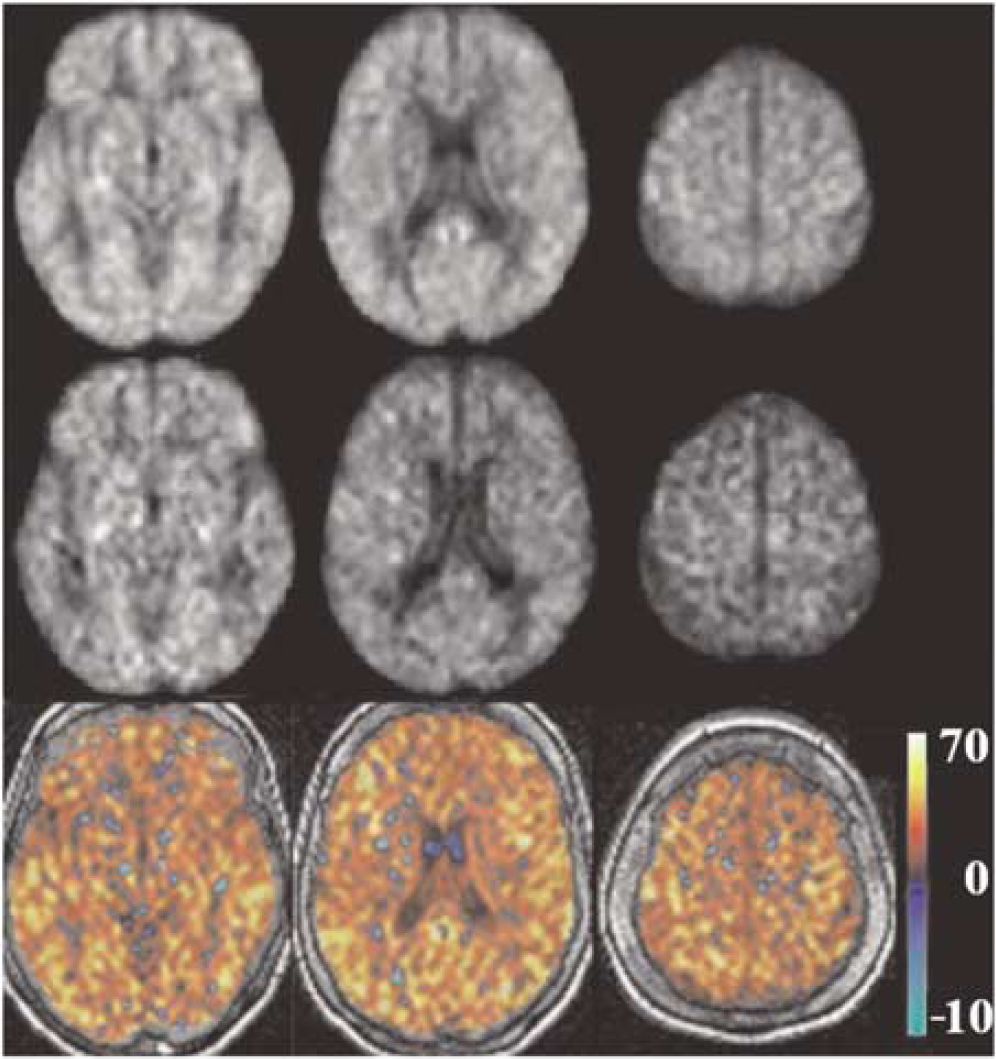
Group average CASL CBF images for HC and AD are shown in the first and second row, respectively, at three axial locations from lower, middle, and upper brain. Corresponding difference images (HC-AD) are shown in the third row. Units in the color bar are in (mL/100 g min).
Global GM CBF was significantly lower in AD compared with HC with mean values of 36.1±7.8 and 62.4±13 mL/100 g min for each group, respectively (t=6.05, P<0.0001). There was no effect of gender in the GM CBF for either group: (t=−0.8, P=0.23) and (t=0.21, P=0.41) for AD and HC, respectively.
Multivariate Analysis
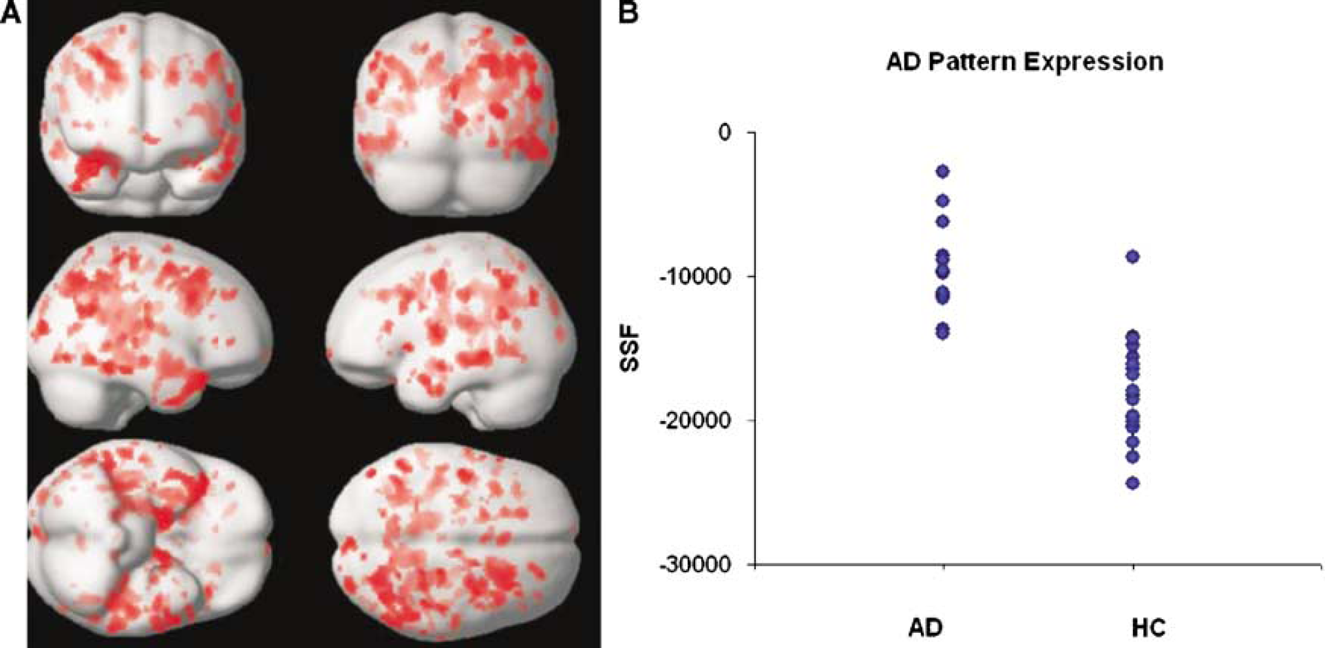
We obtained an AD-related covariance pattern (Figure 2A) whose subject expression achieves significant separation between AD and HC groups (parametric P<0.0005). The permutation test for the group discrimination achieved by the covariance pattern also yielded highly significant results, for both t-statistic and AUC: P(AUC)=0.0002, P(t)=0.0001. The areas showing concomitant decreased flow in the AD subjects are shown in Table 2. No areas of positive loadings (i.e., with concomitant increased flow in AD subjects) were found. Subject expression of the discriminant pattern is shown in Figure 2B. One can appreciate the very small overlap between the two groups and the potential it holds for diagnostic purposes. The ROC curve showed that for an SSF cutoff of −14,100, the covariance pattern was 100% sensitive and 95% specific; AUC was 0.96. Except for one control (79-year-old female, mMMS=53) who was misidentified as AD, all other subjects' group identities were correctly assigned.
(
Areas of the AD-related covariance pattern with significant (P<0.02) negative loadings
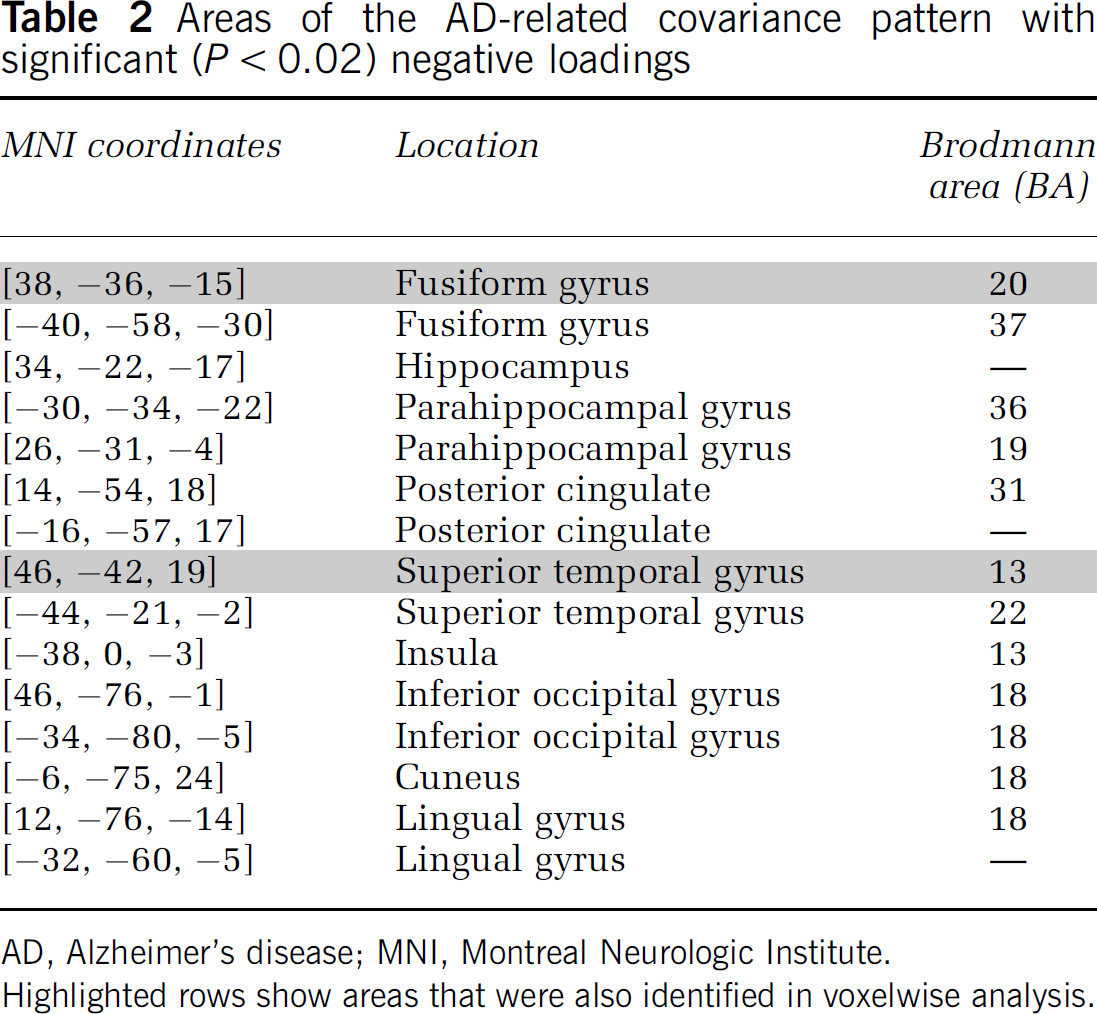
AD, Alzheimer's disease; MNI, Montreal Neurologic Institute.
Highlighted rows show areas that were also identified in voxelwise analysis.
No significant correlation between the covariance pattern and mMMS scores was found. Also, no effect of gender was detected in either group: (P=0.83) and (P=0.08) for AD and HC, respectively.
Region of Interest Analysis
Figure 3 shows CASL CBF mean values of each ROI in AD patients (in blue) and HC (in red). The largest decrease in CBF, 28.3 (mL/100 g min), was found in the right supramarginal gyrus and the smallest, 12.7 (mL/100 g min), in the right parahippocampal gyrus (Figure 3).
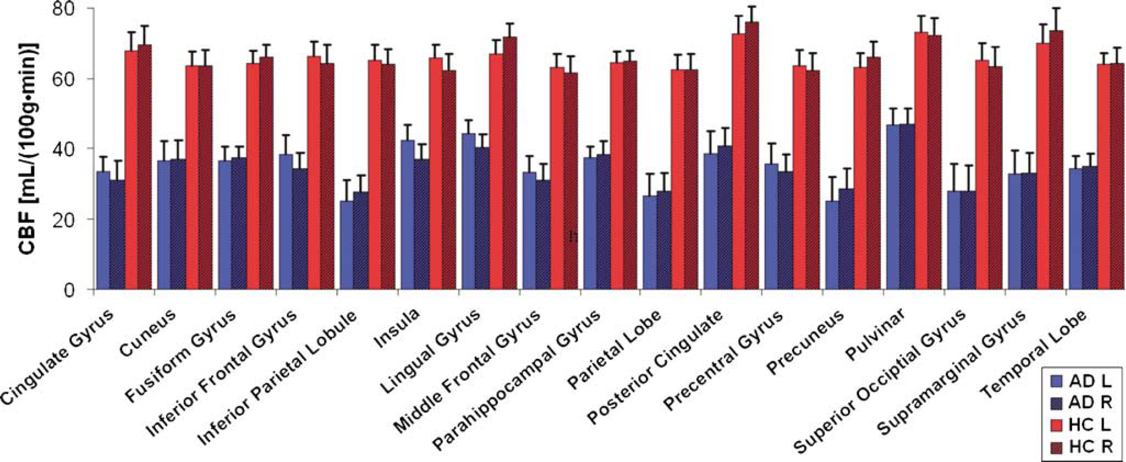
Plot of CBF values (mL/100 g min) versus ROI for AD patients (red, n=12) and HC (blue, n=20). Left (solid) and right (striped) hemispheres are shown separately. Error bars represent ±1 s.e. across subjects in each group.
All ROIs showed a significant CBF decrease in AD patients compared with HC (αcorrected=0.05, P<0.0001). There was no significant difference between the left and right hemispheres for any of the ROIs in either group (paired t-test, P>0.98 for all ROIs).
Areas under the ROC curve for GM and temporal lobe left were 0.94 and 0.93, respectively. Temporal lobe left was selected as the ROI with the highest t-value (t=5.9), whereas GM ROI was selected to assess the power of global CBF changes in discriminating ADs from HCs. The ROC curve for the global GM ROI was used to determine the CBF cutoff for optimum sensitivity and specificity. For a CBF cutoff of 46 (mL/100 g min), 100% sensitivity and 85% specificity was achieved. When the specificity value was increased to 95% to match that of the covariance analysis, the sensitivity decreased to 58% and the CBF cutoff to 35 (mL/100 g min). In this case, in addition to the control subject who was also misidentified by the covariance analysis, five additional AD patients (mean age=76.8±2.1 years, mean mMMS=41.4±12.1, 2 males) were misdiagnosed as controls.
To check whether the observed difference in mean CBF values could be at least partially explained by the difference in the arterial transit time between the two groups, CBF images acquired with PLD=0.8 secs were compared with those acquired with longer PLD=1.0 sec in six AD subjects. The rationale was that if the PLD of 0.8 secs was not sufficiently long for our ascending acquisition, an underestimation of CBF (due to the saturation of labeled spins destined for the upper slices) would be expected in the superior regions of the brain compared to images acquired with longer PLD=1.0 sec. A two-tailed t-test showed no significant difference in precentral gyrus (our most superior ROI) mean CBF acquired with two different PLD values (t=2.2, P=0.58).
The only ROI for which there was a significant positive correlation in AD between mMMS scores and CBF was supramarginal gyrus with R2=0.33 and P=0.05.
Voxelwise Analysis
Figure 4 shows the SPM {T} map for the (HC—AD) contrast (thresholded t=5.73, corrected P<0.05) overlaid on a surface rendering of the brain (Figure 4A) and in a three-dimensional view overlaid on the spoiled gradient recalled of one of the HC subjects (Figure 4B). Areas that showed a significant CBF decrease in AD versus HC are listed in Table 3.
Areas showing significant decrease in CBF (AD versus HC) from voxelwise analysis (corrected, P<0.05)
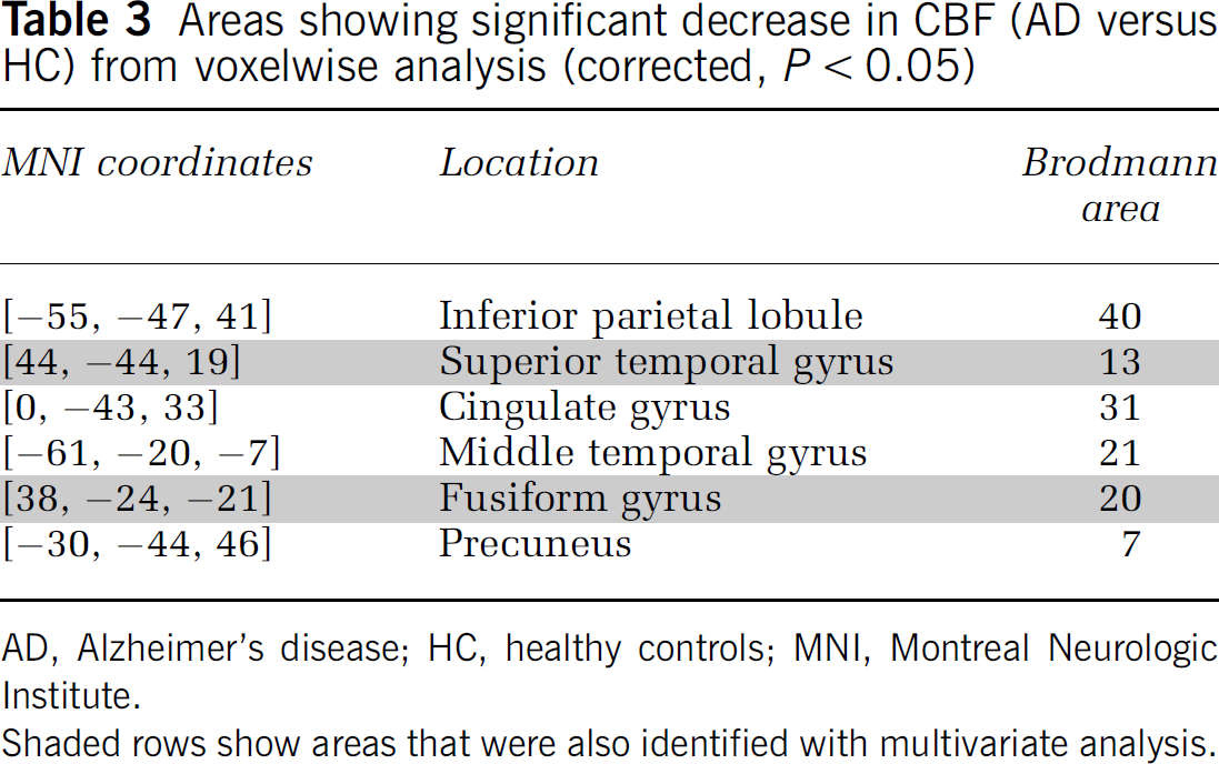
AD, Alzheimer's disease; HC, healthy controls; MNI, Montreal Neurologic Institute.
Shaded rows show areas that were also identified with multivariate analysis.
For the AD group, the regression analysis yielded areas with significant correlation (t>5.7, uncorrected P<0.001) between CASL CBF and mMMS scores in parahippocampal gyrus (BA 28, 30) and middle temporal gyrus (BA 8, 21). There was no voxelwise effect of gender in neither of the groups.
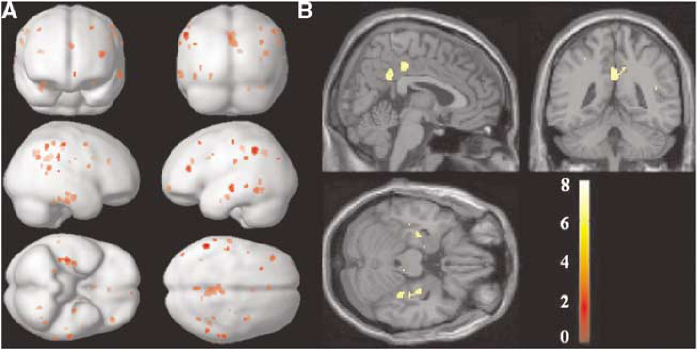
Voxelwise SPM{T}map for the (HC-AD) contrast (corrected, P<0.05) overlaid on (
Supplementary Split-Half Analysis Comparing Voxelwise Univariate and Multivariate Results
One criterion for the evaluation of the relative efficacies of univariate and multivariate approaches is how well their respective findings generalize beyond a particular data set to any other independently acquired data. To this end, we performed an extensive split-half analysis: we arbitrarily split both the AD and HC groups in half and re-derived the AD-related covariance in one half and then forward applied the result to the other half. We performed such split-half analyses 10,000 times and recorded the group-contrast t-statistic and AUC for the derivation sample, but computed it in the replication sample also, that is, in the AD and HC subjects that were left out of the analysis. Although the group strengths for replication and derivation samples are now quite low (6 AD and 10 HC), this demonstration nevertheless gives a sense of the robustness of the covariance approach.
To afford a comparison with univariate techniques, we also recorded the voxel with the highest t-value for the AD—HC contrast in the derivation sample and computed AUC in that sample. The prospective check was then simple: we computed t-contrast and AUC for the same voxel, but in the replication sample.
For simple graphical depiction that enables a quick comparison we plotted histograms of the following ratios for both univariate and multivariate analysis (Figure 5).
AUC ratio=AUC (replication sample)/AUC (derivation sample) t-ratio=t-statistic (replication sample)/t-statistic (derivation sample).
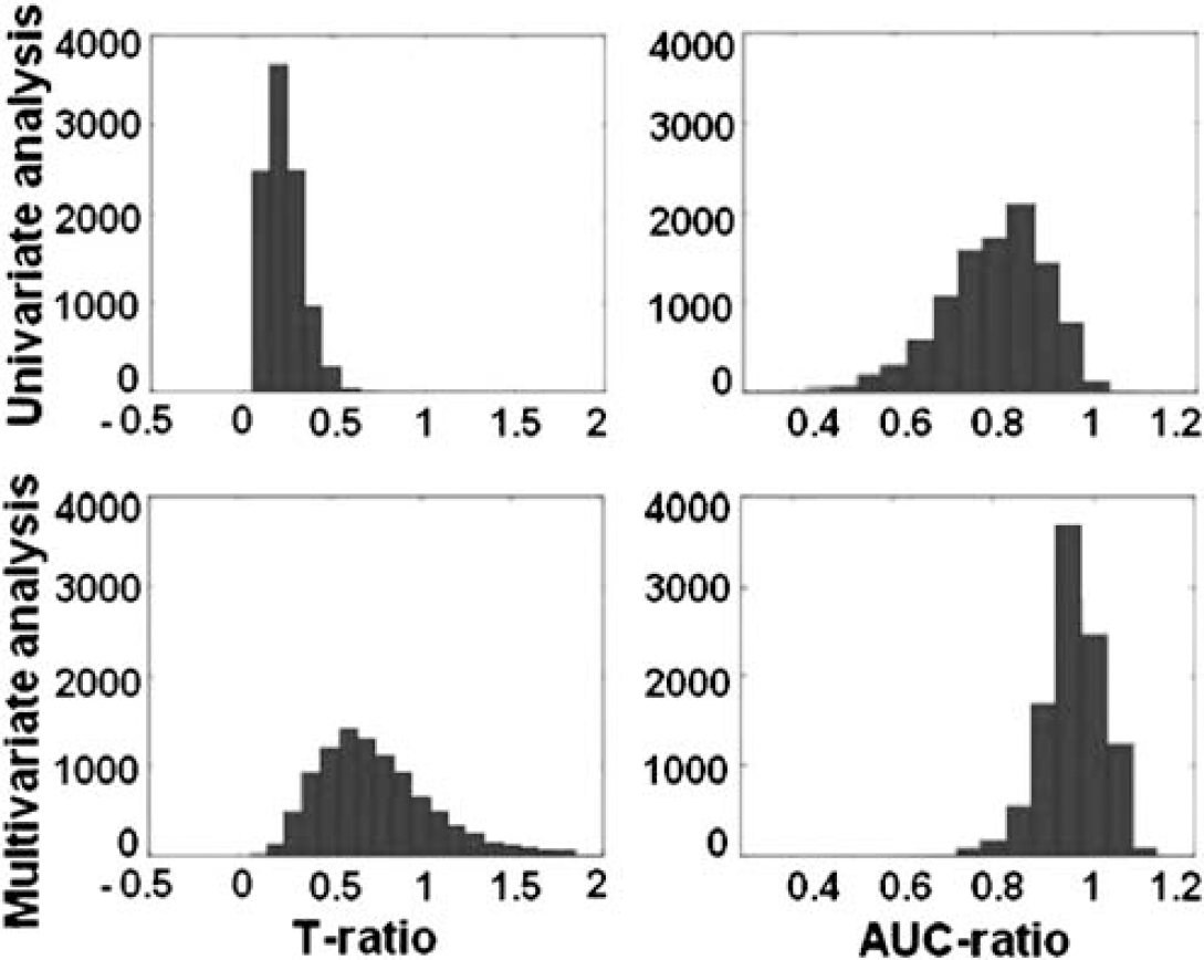
Ratios of t-statistic (left column) and AUC (right column), plotted for both univariate (top row) and multivariate approaches (bottom row). Ratios were defined as the value obtained for the replication sample divided by the value obtained for the derivation sample. Ratios approaching or surpassing unity indicate good replicability.
Good relative replicability implies ratios approaching and possibly surpassing unity. From Figure 5, one can unequivocally discern that the multivariate method is superior in terms of replicability.
This is true not only in relative but also in absolute terms as shown in Table 4, where listed are the mean±s.d. of t-statistic and AUC values in derivation and replication samples for both approaches.
List of mean±s.d. of t-statistic and AUC values for derivation and replication samples from both univariate and multivariate voxelwise analysis
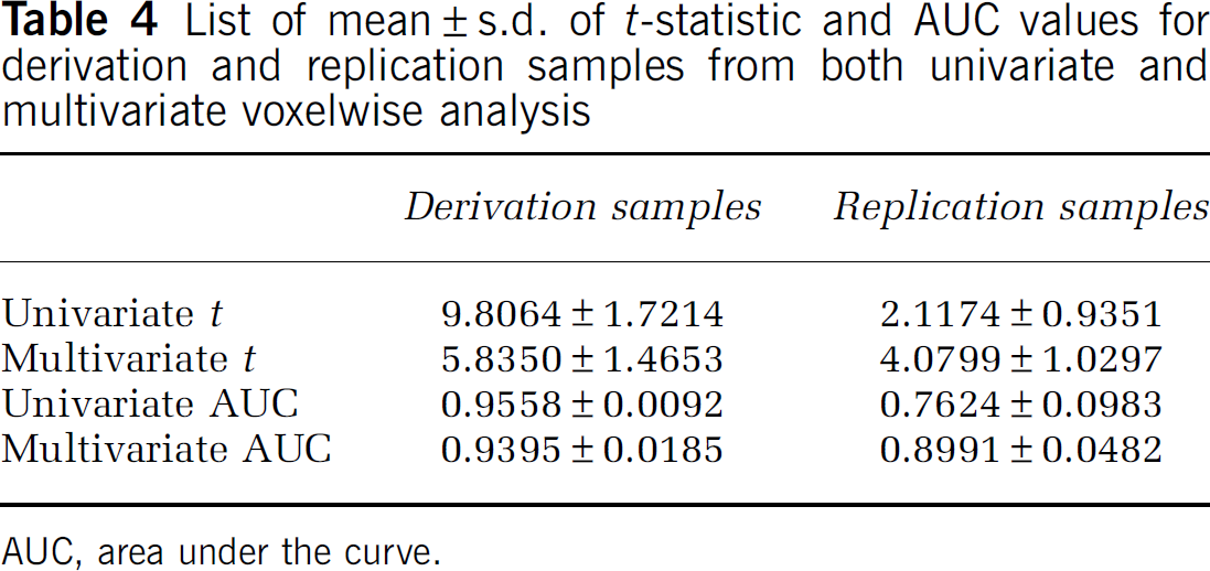
AUC, area under the curve.
The univariate approach results in superior values for the derivation samples, but this cannot be reproduced in the replication samples. Although the univariate t-contrasts are higher than the multivariate ones in the derivation samples, the discriminability as measured by the AUC value is not much different. However, the multivariate approach, while yielding more modest values in the derivation sample, holds up much better in absolute terms in the replication samples.
Discussion
This study is the first to report on whole-brain CASL CBF measurements in AD and the establishment of an AD-related CBF covariance pattern that contrasts AD and controls at baseline. This covariance pattern identified by the multivariate analysis showed very robust group difference in its subject expression. This held not only for the t-test of group mean differences, but also on a subject-by-subject basis, as evidenced by the ROC characteristics of the discrimination (AUC=0.97) misdiagnosing as AD only one out of 20 HCs (a 79-year-old female, mMMS=53). Interestingly, females in the HC group seemed to have a nonsignificantly higher covariance pattern expression than males, that is, showing more ‘AD-like’ behavior. This was not true for the AD group where the effect of gender was highly nonsignificant.
The global GM ROI analysis was also highly discriminatory of the disease-control status, having, however, a somewhat lower specificity than the multivariate analysis (0.85 versus 0.95) for a 100% sensitivity. In addition to the one HC subject misdiagnosed by the covariance analysis, the GM ROI analysis misdiagnosed two additional controls (both females, age 76 and 70 years with mMMS scores of 56 and 54, respectively). Furthermore, when the specificity was increased to match that of the covariance analysis, the sensitivity of global GM ROI decreased to 58%.
The definition of ROIs can be quite arbitrary across studies and tends to vary in both size and tissue content. This makes the generalization of the results across studies quite difficult. For example, in the CASL study by Alsop et al (2000), the ROIs selected were whole-lobe regions from which six out of eight reached significance only at the uncorrected level (P<0.01). In that study, the ROIs were hand drawn potentially including both GM and WM tissue types. In our study, the ROIs were individually defined for each subject using a publicly available atlas and including only voxels with a posterior probability of being GM >0.8.
In general, multivariate analysis might have increased sensitivity compared to univariate analysis even when the disease-related changes in CBF originate in clearly circumscribed foci and spread spatially during the disease course (Scarmeas et al, 2004). Multivariate analysis can detect these subtle, but robust changes, although univariate analysis might experience overly stringent false-positive corrections that tend to ‘correct away’ the true effects (as evidenced by the results of our voxelwise analysis.) The areas pinpointed in the AD-related pattern were mainly located in the medio-temporal lobe and have to face validity in terms of AD pathophysiology (Hoffman et al, 2000), but did not reach significance in the univariate voxel-by-voxel analysis.
Critical to our study would be to compare the predictive utility of the AD-related covariance pattern (obtained through multivariate analysis) with the between-groups mean CBF difference (based on ROI analysis) when applied to the mildly cognitively impaired subjects who have not yet reached the full AD diagnosis. For the multivariate analysis, the expression levels of any AD-related covariance pattern should hold similar predictive powers as our group found with H2O15 PET studies (Scarmeas et al, 2004) where the forward application of the identified covariance pattern to a population with mild to minimal cognitive impairment but no dementia discriminated subjects into those with higher and lower cognitive and functional performance, and predicted differential rates of decline in subsequent follow-up. In contrast to the CASL data presented here, the PET study (Scarmeas et al, 2004) showed no significant differences between groups for the univariate analysis at both the ROI and the voxelwise level. This could be explained by the lack of absolute quantification of the PET data and the need for normalization, which could add to the noise in the data.
One of the advantages of CASL MRI is that it offers a direct and absolute quantification of CBF without the need for injection of expensive and potentially harmful exogenous tracers. One of the confounds, however, of the CASL measurement is transit time, namely, the time it takes for labeled water to reach the tissue in a given voxel. If the average transit time for one group is lower than that of the other, then a difference in CBF will be detected, which cannot be unambiguously attributed to an absolute difference in CBF. To make CASL less sensitive to transit time, Alsop et al (Alsop and Detre, 1996) introduced a delay (PLD) between the end of the labeling pulse and start of the image acquisition. This delay allows more time for blood to arrive and exchange with the tissue. In the presence of vascular disease, a longer PLD would be preferable because transit time could potentially be longer (Alsop and Detre, 1996); the trade off, however, is a decrease in SNR due to T1 relaxation.
In this study, we focused our analysis in the GM where most of the dementia-related changes are expected to occur (Scarmeas et al, 2004). Although we did not explicitly measure the transit time difference between the groups, we conjecture that the transit times were not significantly different based on the following: (1) There was no significant difference in CASL CBF values acquired with two different PLDs, indicating that the shorter PLD we chose for this study was optimum. (2) From the acquisition standpoint, we opted for a longer labeling duration (2.0 secs) and a moderate length PLD (0.8 secs), bringing the total time range from 2.8 secs for the most inferior slice to 3.7 secs for the most superior. (3) Our analysis was based on GM tissue for which the CASL measurement is less sensitive to transit time (Alsop and Detre, 1996) because of the similarity in T1 between blood and GM is ∼1.4 and ∼1.2 secs, respectively (Alsop and Detre, 1996). (4) It is still not clear whether AD is (at least partially) a vascular disease. We screened AD patients for cerebrovascular disease with careful neurologic history and examination. Subjects with history of clinical stroke or imaging evidence of cortical or lacunar infarcts were excluded. Thus, at least clinically, AD patients were not expected to have longer transit time than the controls. However, the transit time could still be a confounder in our findings. White matter abnormalities, which to a certain degree are considered a correlate of subclinical microvessel disease, are more common in AD as compared with healthy (Barber et al, 1999). Their presence, even if not yet visible, would potentially increase the transit times. If the goal is to estimate the absolute depression of CBF in AD, the transit time constitutes a confounder, as the measured decreased would be inflated by a transit time difference. However, if one wants a method that simply distinguishes the two groups at early stages of AD, the effect of transit times would be of little relevance.
In the study by Alsop et al (2000), the CASL implementation was similar to ours but only univariate analysis was applied. The mean GM CBF for the AD group in our study is similar to that of Alsop et al, 36 versus 34 (mL/100 g min), respectively. In contrast, for our HC group, the mean GM CBF observed was higher, 62 versus 38 (mL/100 g min). One of the explanations for this discrepancy could be that we only analyzed voxels with high posterior probability of being GM, whereas in the Alsop et al study, each ROI was hand drawn from an atlas and therefore could have potentially included WM, which is known to have lower CBF than GM (Alsop and Detre, 1996). However, a direct comparison between the two studies is not trivial as in addition to WM inclusion, there are several other differences: first, Alsop et al's study provided only partial coverage of the brain; ours is a whole-brain coverage, which ensures that valid data are obtained from all the subjects but can consequently include more noise in the upper slices. Second, in that study it is not clear whether the slice acquisition time was accounted for in the PLD values used for CBF computation. We correct for slice acquisition time, which ensures that our ROI CBF values are independent of the slice number in the acquisition order. Third, in our ROI analysis, we did not perform any spatial smoothing, whereas CBF images were smoothed with a 12 mm kernel before ROI analysis in the Alsop et al study. Another advantage of our CASL implementation was that it was based on SE-EPI, which allowed for investigation of areas such as inferior region of the frontal lobe and part of the temporal lobe superior to mastoid sinuses that were lacking in the Alsop et al study due to susceptibility effects in gradient echo EPI. In general, however, the data from the two studies are in good agreement with each other, indicating a promising trend toward using CASL as a tool for detection of CBF abnormalities associated with AD.
Although a direct comparison with PASL studies is not straightforward, it is worth mentioning that Du et al (2006) showed good specificity and sensitivity in separating ADs from controls using PASL. Furthermore, this group addressed the issue of the partial volume effect by calculating the ASL signal in each voxel based on posterior probability maps and assuming, from PET data, that WM CBF is 40% lower than GM (Du et al, 2006). Our analysis was similar, in that we too calculated CBF based on posterior probability masks, but circumvented the issue of partial voluming effect by analyzing only voxels with P[GM]>0.8 rather than making assumptions about WM CBF. In general, owing to sensitivity of CASL to transit time effect in WM, any inclusion of this tissue type in CBF computations would lead to an overestimation of CBF (Wang et al, 2003).
Technical advancements in MRI combined with the application of more powerful statistical analysis tools will most likely increase the sensitivity of ASL in detecting CBF changes for early detection, diagnosis, and monitoring of diseases. Theoretically, ASL signal is expected to increase with Bo due to two main factors: an inherent increase in MR SNR with Bo and a longer longitudinal relaxation time of labeled arterial water (Wang et al, 2002). Wang et al (2002) have provided a theoretical framework for the dependence of ASL signal with Bo. They found that in the absence of the T2∗ effect (appropriate for SE-EPI), CASL SNR is expected to increase ∼3 times at 3 T compared with 1.5 T (Wang et al, 2002). Furthermore, using gradient echo EPI, Wang et al (2005) have reported that compared with a standard volume coil, an eight-channel array coil with (twofold) and without acceleration provided a 45 and 56% decrease in intrasubject s.d., respectively.
In conclusion, we have shown the utility of combining CASL perfusion MRI with multivariate and univariate statistical procedures to characterize the baseline CBF differences between AD and HC. Furthermore, we have identified an AD-related covariance pattern that we think holds greater promise in early detection of the disease and prediction of conversion to AD the mildly cognitively impaired than the more standard univariate methods.
Footnotes
Acknowledgements
We thank Mathew Tabert, PhD, for his contribution in recruiting subjects and Hamed Mojahed, MSc, for his help with data acquisition. We are grateful to Xavier Golay, PhD, and Eric Zarahn, PhD, for their invaluable expertise.