Sage Journals: Discover world-class research

Abstract

Knowledge of the blood volume per unit volume of brain tissue is important for understanding brain function in health and disease. We describe a direct method using two-photon laser scanning microscopy to obtain in vivo the local capillary blood volume in the cortex of anesthetized mouse. We infused fluorescent dyes in the circulating blood and imaged the blood vessels, including the capillaries, to a depth of 600 μm below the dura at the brain surface. Capillary cortical blood volume (CCBV) was calculated without any form recognition and segmentation, by normalizing the total fluorescence measured at each depth and integrating the collected intensities all over the stack. Theoretical justifications are presented and numerical simulations were performed to validate this method which was weakly sensitive to background noise. Then, CCBV had been estimated on seven healthy mice between 2% ± 0.3% and 2.4% ± 0.4%. We showed that this measure of CCBV is reproductible and that this method is highly sensitive to the explored zones in the cortex (vessel density and size). This method, which dispenses with form recognition, is rapid and would allow to study in vivo temporal and highly resolute spatial variations of CCBV under different conditions or stimulations.

Keywords

cerebral blood volume mice microvascularisation two-photon laser scanning microscopy

Introduction

Hemodynamic parameters and vascular morphology show characteristic changes in different cerebral disorders like brain tumors, neurodegenerative diseases, traumatic cerebral injuries, ischaemia. Understanding the contribution of hemodynamic parameters such as blood volume, blood flow and vascular permeability in the etiology of diseases will be useful for diagnosis, prognosis and therapy. For instance, angiogenesis is an important stage of tumor development and many therapeutical strategies are developed to inhibit angiogenesis. Consequently, studies of the microvasculature and so tumoral blood volume assessments are crucial to understand the tumor growth process and therapy follow-up. Imaging techniques such as magnetic resonance imaging, positron emission tomography and computed tomography can provide useful information on hemodynamic parameters and vascular permeability (Sanden et al, 2000; Eastwood and Provenzale, 2003; Wintermark et al, 2005; Huppert et al, 2006; Ewing et al, 2006). However, they suffer from relatively poor spatial and/or temporal resolution. Quantitative synchrotron radiation computed tomography has recently allowed high-resolution blood brain barrier permeability and blood volume imaging ((47 μm)² × 0.5 mm in rat) but error bars remain high, especially in the cerebral tissue where the resolution was degraded because of low signals (Adam et al, 2005). The spatial resolution for magnetic resonance imaging vascular parameters assessments on small animal is around 0.23 × 0.47 × 1 mm³ (Tropres et al, 2004). This resolution is a limiting factor for studies on the brain of small animals on which basic researches into potential therapies are performed. Moreover, they rely on mathematical models, which can induce long data postprocessing and make difficult quantitative accuracy (Wintermark et al, 2005). Direct brain imaging with better spatial (micrometric) and temporal resolutions can be obtained using optical techniques (Helmchen and Denk, 2005). Traditional fluorescence confocal laser scanning microscopy allows an imaging depth of about 200 μm in brain tissue with a high spatial resolution (Tomita et al, 2005) and this imaging depth had been extended with the development of multiphoton laser scanning microscopy, which became the main technique for high-resolution in vivo deep imaging (Denk et al, 1990). A imaging depth of 500–600 μm can be obtained currently in the cortex (Helmchen and Denk, 2005) (this covers around 70% of the mouse cortex) and imaging of brain vessels as deep as 1000 μm has been reported (Theer et al, 2003). Previous works on hemodynamic parameters using in vivo two-photon microscopy concentrated on illustrating the vascular anatomy (Kleinfeld et al, 1998), studying changes in capillary blood flow after stimulation (Chaigneau et al, 2003; Kleinfeld et al, 1998) and the redistribution of blood flow after vascular occlusion (Schaffer et al, 2006). The aim of the present study was to develop an in vivo microscopic method to measure mouse capillary cortical blood volume (CCBV). The acronym CCBV is used instead of CBV (for cerebral blood volume) to specify that this measurement is made in capillary rich region of interest, avoiding large vessels. We show how the quantification of CBV can be rapidly derived without morphometric analysis of the blood vessels. The method has been simulated on numerical phantoms for validation and applied on healthy mice. Preliminary results have been partially presented previously (Verant et al, 2004).

Materials and methods

In Vivo Experimental Procedure

All experimental procedures were performed in accordance with the French Government guidelines for the care and use of laboratory animals (licenses 380321, A 3851610004, and B 3851610003).

Swiss NUDE mice (Charles River, France) approximately 5 weeks old, 14 to 24 g in weight were anaesthetized through a face mask with isofluorane (5% for induction of anesthesia and 1.5% for maintenance), 70% N₂O, and 30% O₂. A craniotomy of 3 mm in diameter was carried out on the top of the left parietal cortex (craniotomy center: bregma 2 mm, left 1.5 mm), the bone was removed and the exposed cerebral cortex was protected by an agarose gel, 1% in 0.9% saline solution. One hundred microliters of a 70 kDa fluorescein-isothiocyanate dextran solution (100 mg mL⁻¹, Sigma-Aldrich, FITC-Dextran-70S) or a 70 kDa Rhodamin B isothiocyanate-dextran solution (100 mg mL⁻¹, Sigma, R9379) was injected through the tail vein. (The choice of the dye depends on the nature and especially the emission wavelength of the dye with a smaller molecular weight which can be injected simultaneously for permeability study). Mice were placed on a stereotaxic frame modified to allow a longitudinal rotation of the animal for optimal laser penetration and the brain was positioned under the objective. Core temperature was maintained at 37°C, using warm water circulating through a pad.

No blood analysis was performed during experiments (blood sampling would have disturbed the CCBV measurements). Nevertheless, mice breathed freely during every experiments and woke up at the end.

Microscopy: Two-photon laser microscopy was performed with a confocal microscope (Biorad MRC 1024 scanhead and Olympus BX50WI microscope). The set-up is presented in Figure 1. A 800-nm excitation beam was focused into the mouse brain using a 20 × water-immersion objective (0.95 numerical aperture, Xlum Plan FI Olympus) and the beam was scanned in the x—y plan to acquire 512 × 512 images (1s/image). The variation of the observation depth (z-scan) was realized with the translation of the motorized objective. The incident laser intensity was varied during acquisitions using the rotation of λ/2 quartz window placed in front of two polarizers at Brewster's angle so that the total average power delivered at the surface ranged from 0 to 200 mW. So typically, an energy of 10⁻⁸J is deposed on a surface of around 1 μm² (≈Π*(0.6 μm)²) in the focal region. For the experiments carried here, the confocal configuration was not used here but non-descanned fluorescence was collected with two added external photomultiplier tubes. A filter cube (HQ535-30, 585DCXR, HQ620-60) in front of the photomultiplier tubes separated the red fluorescence from the green one so that two dyes (with different emission wavelengths and different molecular weights, for permeability studies for instance) could be simultaneously observed. Image acquisition and reconstruction were performed by the Biorad acquisition system and images were analysed using Image J (NIH free software available on http://rsb.info.nih.gov/ij/) and Delphi5 macro.

Figure 1

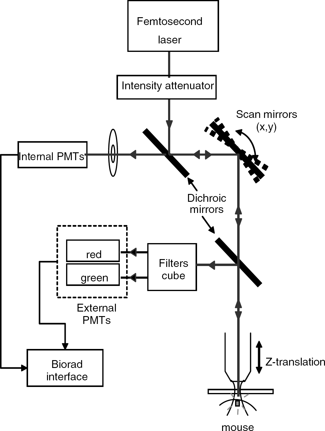
Schematic representation of the microscopy set-up.

The objective was chosen according to the studies of Oheim et al (2001) and Beaurepaire et al (2001). They showed that fluorescence collection and consequently penetration depth could be optimized by using a low magnification (×20), high-numerical aperture objective (0.95) and by underfilling the back aperture of the objective. Moreover, fluorescence was collected through external photomultiplier tubes without any spatial selection so as to collect the maximum of fluorescence generated at a given position of the beam focus (Helmchen and Denk, 2005). The spatial resolution of our set-up is less than 0.6 μm in the lateral extent and less than 6 μm in the axial extent (see paragraph ‘Image processing’).

Image acquisition: Planar scans of fluorescent intensity I(x, y, z) were acquired at successive depths in the cortex (with (x, y z) the coordinates of the laser focal point). The z-step between scans was 2 μm. The collection time of a 200-μm-thick stack is around 2 mins. To counterbalance the attenuation of the exciting light and the emitted fluorescence when getting deeper in the tissue, the intensity of the laser was manually increased as the depth increased for collecting the highest fluorescent signal as possible without saturating any pixel of the image. The offset of the photomultiplier tubes was optimized to avoid artificial signal background during the acquisitions.

Image Processing for Cerebral Blood Volume Measurements

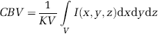
Principle: The cerebral blood volume (CBV) is the fraction of the total observed volume occupied by the blood in the vessels:

C B V = \frac{V_{b l o o d}}{V_{o b s e r v a t i o n}}

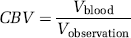
It can also be expressed by the following integral:

C B V = \frac{1}{V} \int_{V} F (x, y, z) d x d y d z

(1)

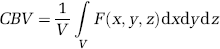
with V being the observed volume and F(x, y, z) the ‘blood vessels function’

F (x, y, z) = {\begin{cases} 1 & if (x, y, z) belongs to a blood vessel \\ 0 & otherwise \end{cases}

In all cases, we assume that the fluorescent dyes are confined and uniformly distributed inside the blood vessels with a concentration C.

If the laser were confined to an infinitely small volume at the focal point, the images would be perfectly digitalized and the CBV expression would take an intuitive form

C B V = \frac{N_{on}}{N}

(2)

with N being the total number of pixels in the volume of interest and N_on the number of ‘switched-on’ (fluorescent) pixels. Indeed, a pixel is either ‘on’ when the pixel belongs to a vessel or off otherwise.

In this case, the detected intensity of two-photon fluorescence (for a laser focal point of coordinates x, y, z) would be proportional to the product of F(x, y, z) with the local fluorescent dye concentration in blood vessels C(x, y, z) = C and with the square of the laser excitation intensity at this point L(x, y, z):

I (x, y, z) = α F (x, y, z) C L^{2} (x, y, z)

(3)

where α is the efficiency of fluorescence generation and collection. If the laser intensity L(x, y, z) = L₀ and α stay constant over the volume of interest, the above expression becomes

I (x, y, z) = K F (x, y, z) with K = α C L_{0}^{2}

In these conditions, the ‘3D image’ I(x, y, z) maps F(x, y, z) and it gives access to the CBV in that Expression (1) becomes

C B V = \frac{1}{K V} \int_{V} I (x, y, z) d x d y d z

(4)

In fact, the laser excitation (and thus fluorescence emission) is confined to a small ellipsoidal volume around the focal point where the photon density is high enough to generate two-photon absorption events (Rubart, 2004). The collected intensity for a given focalization of the laser is then the convolution of the two-photon intensity excitation (two-photon Point Spread Function) with the distribution of the fluorescent dyes in the volume of interest (which corresponds to the distribution of blood). The convolution induces a kind of blurring of the images (pixels are ‘contaminated’ by neighbors, especially above and below) but the sum of intensities over all pixels remains unchanged. So it can be demonstrated that the relation between CBV and the fluorescent intensities does not depend on the extents of the PSF and Expression (4) is still valid (see Appendix A, point 1).

Relation (4) can be generalized for digitized images under the condition that

either the voxel size (pixel size × step in z) is far smaller than the extents of the two-photon PSF (Point Spread Function) (condition 1)

or the two-photon PSF extents are inferior to the voxel dimensions, negligible in front of the dimensions of the objects of interest too (condition 2).

Then Expression (4) becomes

C B V = \frac{1}{K V} \sum_{(i, j, k) \in V} I (i, j, k) = \frac{⟨ I ⟩}{K}

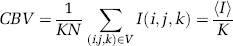
where (i, j, k) are the voxels's identifiers, N is the total number of pixels in the volume of interest and 〈I〉 the average intensity over all the pixels of the stack.

Moreover, if the extent of the PSF is smaller than the characteristic size of the vessels, when the PSF matches well a blood vessel, we have I(I, j, k) = K = I_max with I_max being the brightest intensity acquired over the scan with a constant laser excitation intensity (see Appendix A, point 2). Such a brightest zone exists (condition 3) in each planar scan when a large plunging vertical vessel goes through the whole stack. Then the CBV of the stack is given by CBV = 〈I〉/I_max.

The assumption that the laser excitation intensity and the efficiency of fluorescence collection stay constant over the volume of interest, made above to simplify the presentation, is not realistic because of the strong light scattering and attenuation by biological tissues. During a stack acquisition, this scattering brings an additional z-dependence of excitation and fluorescence collection and we have K(z)=I_max(z)=α(z)CL₀²(z). Consequently, the collected intensity must be normalized at each depth with the maximal intensity I_max(z) and then the CBV is given by:

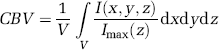
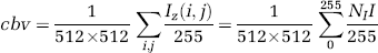
C B V = \frac{1}{V} \int_{V} \frac{I (x, y, z)}{I_{max} (z)} d x d y d z

(5)

and for digitized acquisition

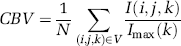
C B V = \frac{1}{N} \sum_{(i, j, k) \in V} \frac{I (i, j, k)}{I_{max} (k)}

(6)

This discretization can be done under the supplementary condition that the characteristic length of attenuation is far larger than the step size in z (condition 4).

Consequently, the above expression shows that, under a few restrictive conditions, the CBV can be extracted from a stack by summing all voxel intensities, after normalization of these intensities over each planar scan with the brightest intensity of the corresponding scan. The procedure for extracting CBV from an acquisition is now presented below.

Image processing: The characteristics of the two-photon PSF of our set-up was less than 0.6 μm in the lateral extent (full-width at half-maximal emission intensity) and less than 6 μm in the axial extent (Verant et al, 2004).

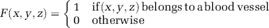
This corresponds to the spatial resolution. The voxel size is (1.15 μm)² × 2 μm; thus, the lateral extent fulfilled condition 2 (the vessel diameter is larger than 3 μm) but the axial extent did not totally fulfill the first condition. However, capillaries are structures with cylindrical symmetries, oriented in the 3D dimensions of space in our in vivo acquisitions (see Figure 2) and consequently errors induced by the discretization are assumed to neutralize one another. Condition 3 was realized too as at least one vessel perpendicular to the planar scans (plunging and vertical arterioles or venules) can be found in each stack: even if the PSF axial extent is larger than the vessel sizes, the focal volume matches well with a vessel. This allows renormalization of each planar scan with the maximal intensity of this scan. At last, the typical attenuation length in the cortex varies between 120 and 220 μm in the rat (Kleinfeld et al, 1998); consequently, the condition 4 should be verified even in the mouse where the attenuation length is in the same order (we found between 50 and 200 μm, data not shown). All conditions were fulfilled, which justified the use of Expression (6).

Figure 2

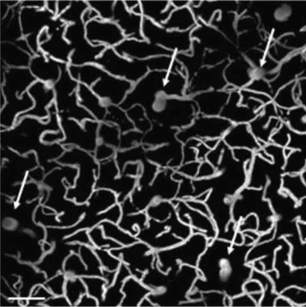
z-projection of 51 images acquired from 100 to 200 μm in the left parietal cortex of a mouse injected with 100 μl of a 100 mg mL⁻¹ FITC-Dextran solution. This is a typical stack from which CBV is estimated. Note the plunging vessels (white arrows), which are essential for the calibration of the light intensity per image. Scale bar corresponds to 100 μm.

The image processing was carried out in several steps.

First, the background, due, for instance, to extravascular fluorescent dyes diffusing mainly from traumatized areas by the surgery, was subtracted on each planar scan using the algorithm ‘Rolling Ball’ of Image J (Sternberg, 1983). This algorithm allows to subtract a uniform background or a non-uniform one which varies slowly in space. The characteristic size below which intensity variations must not be eliminated is fixed by the ‘Rolling Ball Radius’. In our case, it had been fixed at 23 μm by comparison with the distribution size of the vessels (<20 μm in our in vivo images). According to Lichtenstein et al (2003), who studied cytosqueleton network, this algorithm is the most effective one for images with ‘filamentous structures’.

Each planar scan was then convolved with a Gaussian function (FWHM 2.3 μm or 2 pixels) to eliminate saturated pixels due to artefacts, which could introduce errors in the normalization.

The normalization of each planar scans was made by scaling the intensities of each scan between 0 and 255 (for an 8-bit acquisition) using the ‘enhance contrast’ process of Image J.

An average z-projection (I_z(i,j)=1/n∑_k=0ⁿI(i,j,k) with n being the number of images in the stack and the histogram (giving the number of pixels of a given intensity) of the resulting image were performed. With this histogram, the presence of an additional averaged background due to acquisition and exterior noises could be detected and determined. A global correcting offset could be subtracted on the intensity of all pixels before calculating the CBV. For instance, if 10% of the pixels in the whole stack was saturated, it would induce an additional average uniform background on the z-projection of 25 in intensity level. All over this paper, this offset determined on the z-projection by the experimentalist and subtracted (or not) will be named the ‘global correcting offset‘.

The CBV was calculated according to Expression (6)

c b v = \frac{1}{512 \times 512} \sum_{i, j} \frac{I_{z} (i, j)}{255} = \frac{1}{512 \times 512} \sum_{0}^{255} \frac{N_{I} I}{255}

with N_I being the number of pixels with a intensity value I (given by the histogram of the z-projection). 255 corresponds to I_max value fixed by the normalization.

Numerical Simulations

To validate our procedure, numerical simulations were performed. Our ‘computer phantom’ consisted of cylinders representing vessels filled with dye solution randomly distributed in the three directions of space in a cube of 512 × 512 × 512 pixels. The cylinder radii varied randomly between two chosen values (typically 6 to 10 pixels which corresponds to 3 to 5 μm). All pixels inside the cylinders had identical intensity coded on 8-bit (bright white: intensity 200) and pixels outside are black (intensity 0). Figure 3 presents one image of a simulated stack (Figure 3A) and the z-projection of the same simulated stack (Figure 3D).

Figure 3

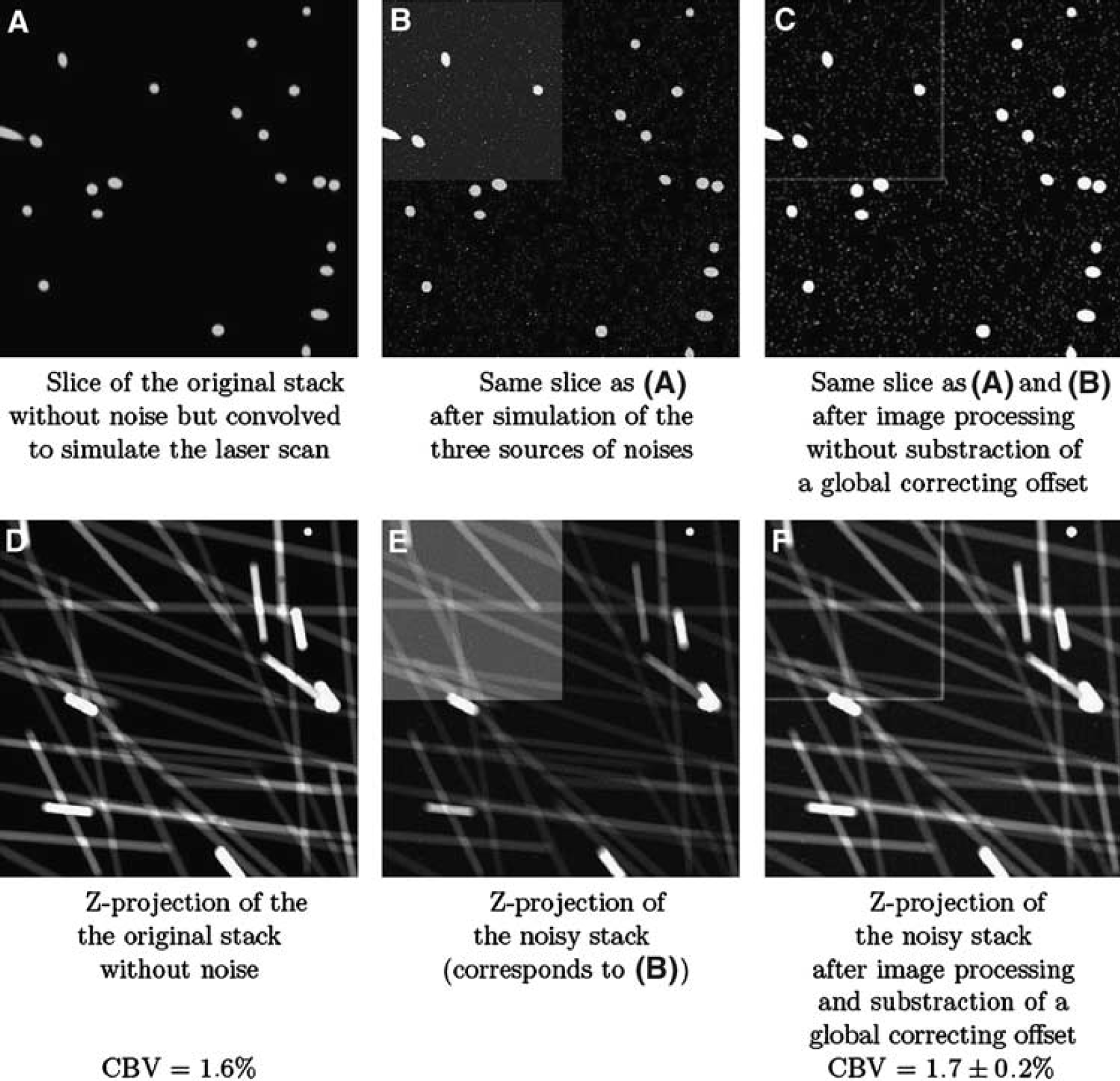
Numerical simulation of capillary distribution inside a cube of 512 × 512 × 512 pixels, 8-bit (256 grey levels) intensity coded. A few steps of the study of the effects on noise simulation and of the image processing to calculate the CBV are illustrated here.

The scan of the laser was simulated by a convolution with a theoretical two-photon PSF (taken as a Gaussian—Lorentzien function with the corresponding characteristics of our set-up), whose intensity maximum decreased with increasing z (depth). Different sources of noise had been simulated so as to explore the efficiency of the image processing for CBV determination:

(a)

An offset could be added to pixel intensities on one-fourth of the stack to simulate dye leakage (example in the upper left corner of Figure 5), a variation of depth observation over the scan.

(b)

The noise from the acquisition process and especially the photonic noise could be simulated with a Gaussian distribution of the fluorescent pixel intensities. The standard deviation was estimated at 15 (for 8-bit coded images) from images acquired on a sample made of an FITC-Dextran homogeneous solution.

(c)

A ‘salt noise’ could be simulated with randomly saturated pixels.

Figure 4

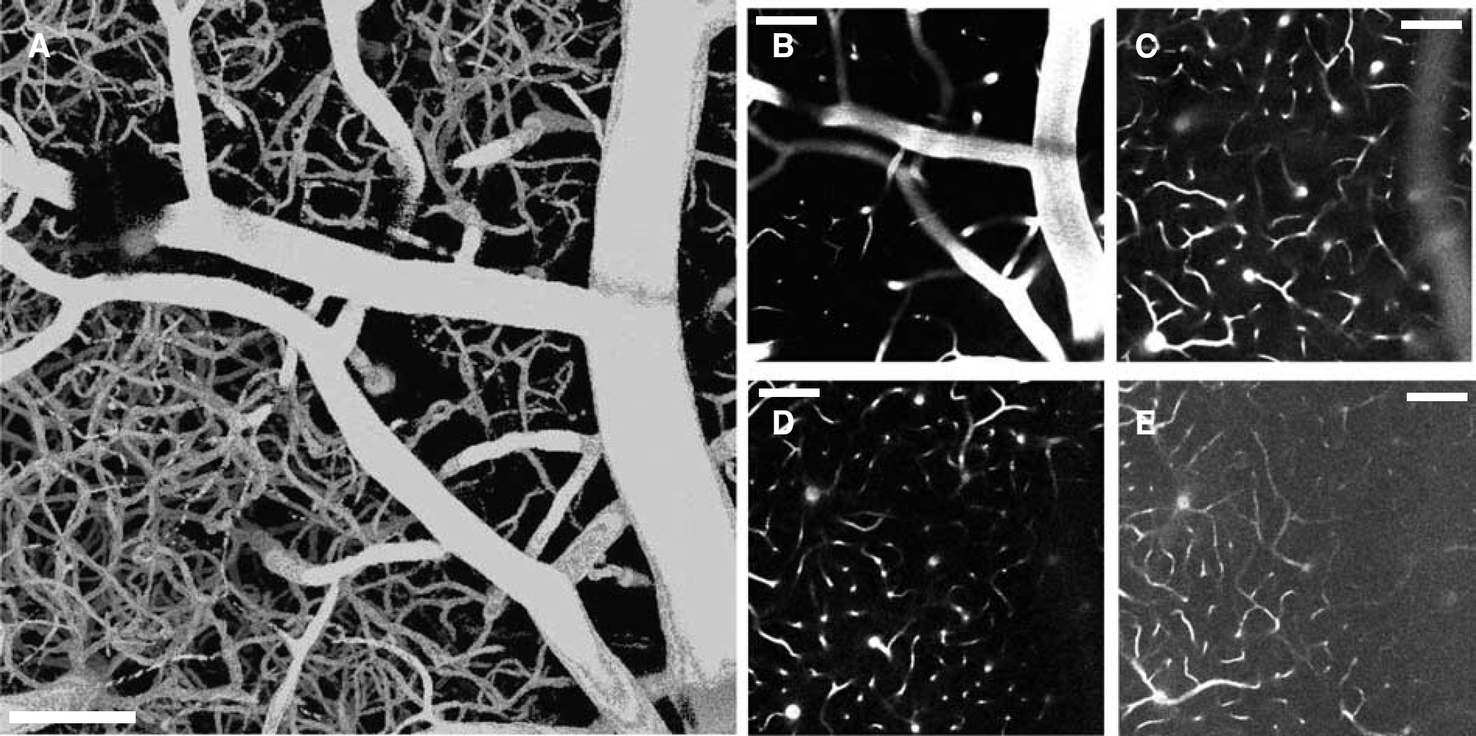
Stack of 121 images acquired in vivo from 0 to 600 μm in the left parietal cortex of a nude mice injected intravenously with 100 μl of a Rhodamine B-Dextran solution (100 mg mL⁻¹). (A) 3D reconstruction of the stack. B, C, D, E) Scans acquired at different depths: 40 μm (b), 150 μm (c), 300 μm (d), 600 μm (e). The scale bar corresponds to 100 μm.

Figure 5

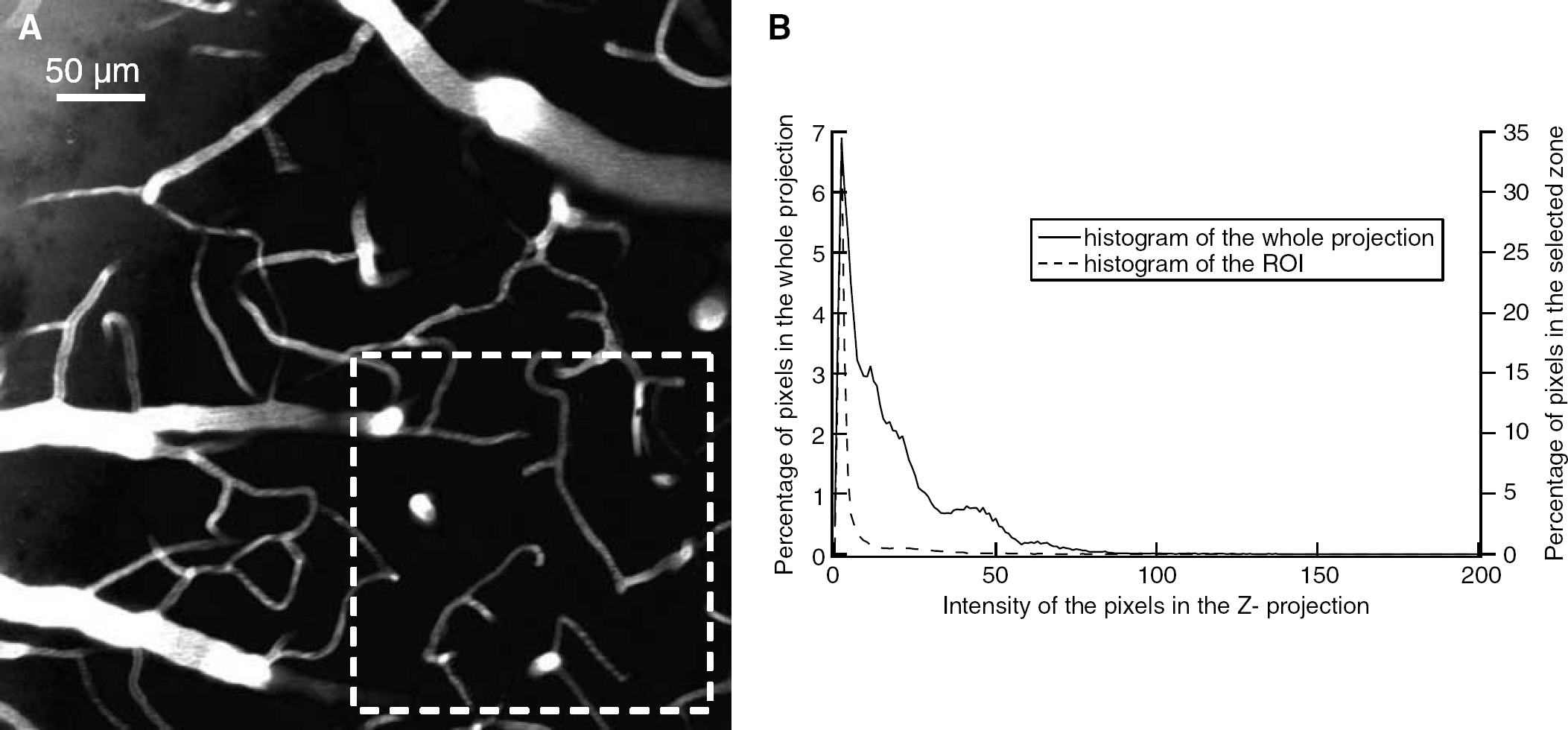
The CBV depends on the explored zones. (a) Z-projection of 101 images taken from the dura up to 50 μm in the cortex of a nude mice injected with 100 μL of an FITC-Dextran 70 kDa solution (100 mg mL⁻¹). The CBV calculated on the whole image is 6% and on the ROI (zone delimited by the white square) is 2.5%. (B) Histogram of the proportion of pixels of a given intensity in the Z-projection.

The effects of each steps of image processing had been explored on this ‘computer phantom’ and are presented in the next paragraph.

Results

Numerical Simulations

Before applying our method to measure in vivo CBV on healthy mice, we tested it on computer phantoms described above. Our phantom had 40 vessels representing capillaries whose radii varied between 3 and 5 μm with an original CBV of 1.6%. This is representative of our in vivo experimental stacks (for instance, the average radius on 30 capillary sections measured on the z-projection of the stack presented in Figure 2 is 4.1 ± 0.7 μm).

If all steps of the image processing presented above are carried out on the original stack, the same CBV are found (see Figures 3A/3D).

When a Gaussian noise is added on the capillaries (noise b) with standard deviation (s.d.) of 15, a CBV of 1.6% is found.

If a Gaussian noise (s.d. of 15) was simulated on the capillaries and an offset was added afterwards on one-fourth of the stack (noise a), the calculated CBV was 1.6%. This photonic noise (noise b) had been only simulated on the capillaries because the intensity of a background due to a dye leakage was very low compared with intensities in capillaries so we neglected the photonic noise on this kind of background.

In all these cases, no ‘global correcting offset’ was subtracted before calculating the CBV (part of step 4 of the image processing).

It was necessary to subtract a global correcting offset when a ‘salt noise’ (noise c) was generated. When 1% of the pixels were saturated on a stack with additional background on one fourth (noise a) and Gaussian distribution of the capillaries intensities (noise b), we found a CBV of 1.7% ± 0.2%. The error bar depends on the value of the ‘global correcting offset‘. Figures 3B/3E correspond to the stack before image processing and Figures 3C/3F after image processing.

Similar results were obtained if the laser scan was simulated before the addition of any kind of noise.

The same ‘step by step study’ was carried out on a numerical phantom whose vessel radii varied between 5 and 8 μm and original CBV was 3.4%. We had similar results and in the more constraining case, we found a CBV of 3.2% ± 0.3% (depending on the value of the global correcting offset).

So, the simulation results are very close to the real values in most of the cases.

In Vivo Acquisitions

This method was then applied to measure the CCBV of healthy mice on in vivo acquisitions. Examples of acquisitions are presented in Figures 2 and 4. In our experimental conditions, vessels as far as 600 μm below the dura were imaged (see Figure 4). However, the maximal observation depth often decreased with the age of mice because of an increasing brain tissue diffusion (Oheim et al, 2001; Helmchen and Denk, 2005). Large vessels—including meningeal vessels—were mainly present at the surface and, when getting deeper, the penetrating vessels divided in numerous branches. The density of capillaries increases from the surface, where capillaries are sparse, down to 40 to 50 μm and then stay constant on the observing depth (see Figure 4).

No compression of the cortical surface was induced by the water-immersion objective lens thanks to a large working distance (2 mm) and the presence of free water drop.

In none of the experiments did we detect the effects of the laser beam scan on the blood circulation such as local thrombosis or any kind of photoactivation. Although we cannot exclude local tissue heating or photodamage, the local heating is limited by the perfusion of blood and the very short pixel dwell time (2.7 μs/pixel). The length of experiments (several stacks are acquired on the same mouse) was only limited by the decreasing of plasmatic dye concentration (within 2 or 3 h).

CCBV of Healthy Mice

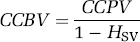
The CCBV has been determined on seven healthy mice. Several stacks of 100 μm were acquired between 50 and 200 μm under the dura of each mouse. Given the fact that our dyes are plasmatic tracers, our method gives access to the capillary cortical plasmatic volume (CCPV), which must be corrected from the haematocrit. Because small vessels are mainly concerned, an haematocrit of H_SV = 30% (Bereczki et al, 1993) has been used to correct the values as follows:

C C B V = \frac{C C P V}{1 - H_{SV}}

The results are given in Table 1. For each mouse, the average CCPV value calculated over the different stacks and the corresponding CCBV is given with the standard deviation over the values (the uncertainty due the method had not been taken into account). The CCBV varied between 2% ± 0.3% and 2.4% ± 0.4%.

Table 1

Results of CCBV estimation on 7 mice

Number of stacks	CCPV		CCBV
Number of stacks	in %	in ml/100 g	CCBV
15	1.4 ± 0.2	1.3 ± 0.2	2 ± 0.3
7	1.7 ± 0.7	1.6 ± 0.6	2.4 ± 0.9
5	1.6 ± 0.3	1.5 ± 0.3	2.3 ± 0.4
10	1.7 ± 0.2	1.6 ± 0.2	2.4 ± 0.4
7	1.7 ± 0.3	1.6 ± 0.3	2.4 ± 0.4
8	1.4 ± 0.1	1.3 ± 0.1	2 ± 0.1
8	1.4 ± 0.1	1.3 ± 0.1	2 ± 0.1

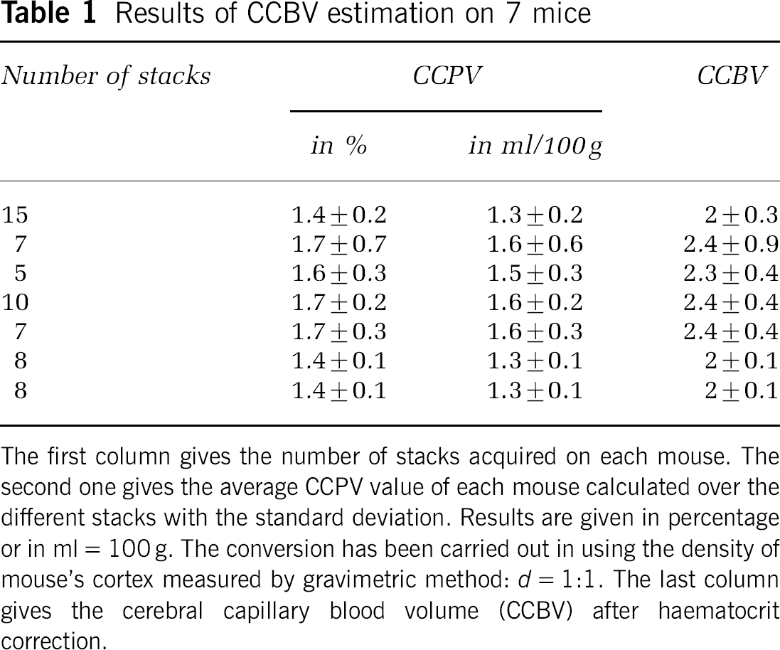
The first column gives the number of stacks acquired on each mouse. The second one gives the average CCPV value of each mouse calculated over the different stacks with the standard deviation. Results are given in percentage or in ml = 100 g. The conversion has been carried out in using the density of mouse's cortex measured by gravimetric method: d = 1:1. The last column gives the cerebral capillary blood volume (CCBV) after haematocrit correction.

The measures made with the method are reproductible (see Table 2). The CCPV (and consequently the CCBV) depended on the explored zone (see Table 2, mouse 4), especially whether it contained large vessels or not. For example, in the acquisition whose projection is presented in Figure 5, taken from the dura up to 50 μm in the cortex, the CCPV varies from 6% when the CCPV is calculated in the whole field of view to 2.5% when it is calculated in the ROI (in the right down corner of the scan where large vessels are rare). The difference comes from the higher proportion of large vessels that can be detected on the histogram (Figure 5B) by a higher proportion of high-intensity pixels in the z-projection compared with the histogram of the more homogenous ROI.

Table 2

Reproducibility of CCPV measurements

Mouse 1	Mouse 2	Mouse 3	Mouse 4
1.5% ± 0.2%	1.4%	1.6% ± 0.2%	2.3% ± 0.4%
1.6% ± 0.2%	1.4% ± 0.2%	1.65% ± 0.2%	1.7% ± 0.2%
1.5% ± 0.2%	1.4% ± 0.2%	1.9% ± 0.2%	1.9% ± 0.3%
	1.5% ± 0.2%	1.9% ± 0.2%	1.9% ± 0.3%
		1.9% ± 0.2%

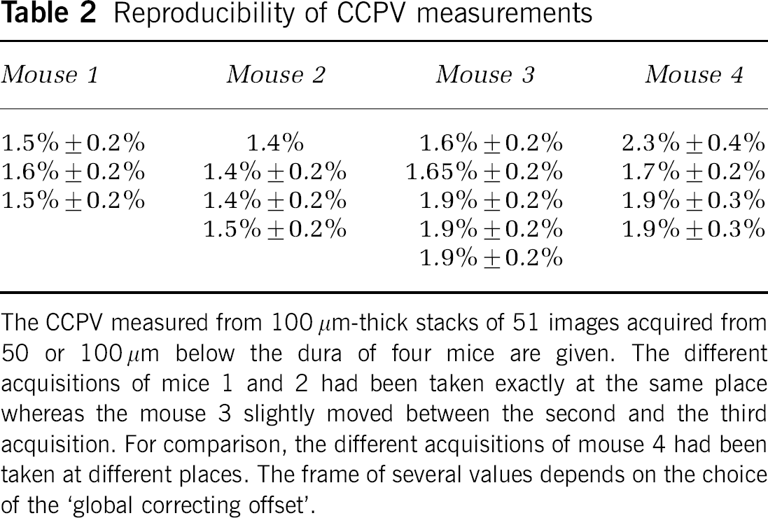
The CCPV measured from 100 μm-thick stacks of 51 images acquired from 50 or 100 μm below the dura of four mice are given. The different acquisitions of mice 1 and 2 had been taken exactly at the same place whereas the mouse 3 slightly moved between the second and the third acquisition. For comparison, the different acquisitions of mouse 4 had been taken at different places. The frame of several values depends on the choice of the ‘global correcting offset‘.

Discussion

In this study, we present a method to measure rapidly the cerebral blood volume without morphometric analysis of the blood vessels. We first validated this method on numerical phantoms and in a second step, we used it to evaluate the CCBV of healthy mouse. To our knowledge, it is the first report on in vivo CCBV imaging with such a high spatial resolution.

The computer simulation was a first step to validate our method: it appeared to be weakly sensitive to noise if the variations were smooth, which was the case in our in vivo acquisitions. Indeed, the main difference between the estimated CBV and the original one occurred when the noise level varied too quickly to be eradicated with the ‘rolling ball’ process (case D in the numerical simulation) and were not homogeneous enough all over the stack to be suppressed by the global correcting offset. So the frontier that remained on Figures 3C/3F could not be eradicated by the ‘rolling ball’ process because of a too abrupt intensity variation; such variation was not realistic and did not occur in our in vivo acquisitions. In all other cases, the calculated CBV was very close to the original one. Moreover, the in vivo measures on healthy mouse are reproductible.

The variation with depth of the efficiency of fluorescence generation and collection is taken into account through the normalization of every image in a scan. This can be done because the cortical surface curvature can be ignored (errors < 10%) for horizontal distances from the calibration pixel up to 2 mm, which is greater than the XY amplitudes of the scan described and thus the depth is constant in one image. The efficiency may vary over a planar scan because of large superficial vessels that absorb a part of the emitted fluorescence: the absorption coefficient of the blood and especially the haemoglobin is about one order higher than the typical one of brain tissue (400 cm⁻¹ compared to about 50 cm⁻¹ at 630 nm (Kleinfeld et al, 1998)). The last value must be taken with caution as it depends on the age of the mouse and its physiological state. This can lead to a slight underestimation of the CCBV if the ROI is located below large vessels. In the results presented in Table 1, these shadowing effects had been avoided by choosing manually the explored zones.

Our dyes are plasmatic tracers that is why our measurements (giving access to the CCPV) should be corrected for the haematocrit in order to have a better comparison with values of CBV given in the literature. The haematocrit has values depending of the size of the vessels, ranging from 0.42 for large vessels to 0.3 for small vessels ((Bereczki et al, 1993)). Because large vessels were avoided in the ROI where measurements are made, a single hæmatocrit (H_SV = 30%) can be used for correction (it is not necessary to consider an average haematocrit as pointed out by Adam et al, 2005).

First of all, to our knowledge, no value for the mouse is given in the literature: the CCBV values obtained by this microscopic method are comparable with values given by other methods that are performed on rat. However, the given values in the literature are heterogeneous and quantitative comparison is hazardous (Adam et al, 2005). With Synchrotron Radiation Quantitative Computed Tomography (Adam et al, 2003), a mean CBV of 2.1 ± 0.38 mL/100 g in the parietal cortex of rat is given; Tropres et al (2004) and Dunn et al (2004) reported CBV values of 4.3% ± 0.7% and 3.14% ± 0.32% respectively in the parietal rat cortex, using magnetic resonance imaging techniques with a super paramagnetic contrast agent. According to Adam et al (2005), quantitative magnetic resonance imaging CBV values for gray matter in healthy rat brain range from 1.65 to 4.1 mL/100 g. With stereological methods, Schlageter et al (1999) found a CBV of 2.1 ± 0.9 mL/100 g in the grey matter of rats (in comparison with 1.2 ± 0.3 mL/100 g for the white matter). On the one hand, the first two methods (computed tomography and magnetic resonance imaging) are performed in vivo but have a poorer spatial resolution (respectively 0.047 × 0.047 × 0.5 mm³ in the best cases (Adam et al, 2005) and 0.23 × 0.47 × 1 mm³, acquisition in 40 mins (Tropres et al, 2004)) and they take into account all vessels. On the other hand, the stereology is performed ex vivo on physical slices and gives access to numerous morphometric parameters. In addition, Schlageter et al took into account only the microvasculature (diameter inferior to 15 μm). However, the effects of death, fixation and slicing on the microvasculature are not well described.

Moreover, the comparison with other values found in the literature is limited by the variability of CBV within the explored brain areas (Vanzetta et al, 2005) and our method is highly sensitive to vessels size and density because of its high resolution.

The variability of the CCBV values on one mouse is mainly due to the variability between the explored zones, but it can be due to errors introduced by the image acquisition and processing too. However, numerical simulations showed that the image processing is quite robust to different sources of noise. Another cause of variability that made hazardous comparison between CCBV values of different mice is the intrinsic biological variability between mice (age, weight, physiological conditions during anesthesia.).

Many of these causes of variability can be eradicated by following temporal effects on the same mouse and at the same place (with a permanent cranial window for instance). Protocols for long-term studies of the microcirculation with a closed cranial window are detailed in Gaber et al (2004).

The concern of this paper was to show the feasibility of this method which dispenses with form recognition (segmentation is not necessary) and consequently is rapid and could be automated. The increase of the incident intensity can be automatically increased and all steps of the image processing can be carried out on line during the experiments. This would allow to follow variations of CBV with high temporal and spatial resolutions under different conditions or stimulations such as normocapnic and hypercapnic cycles, cerebral ischemia, drugs, and radiotherapeutic treatments.

Footnotes

Acknowledgements

The authors thank Jonathan Coles and François Estève for helpful and useful discussions.

Appendix A

References

Adam

Elleaume

Le Duc

Corde

Charvet

Tropres

Le Bas

Esteve

(2003) Absolute cerebral blood volume and blood flow measurements based on synchrotron radiation quantitative computed tomography. J Cereb Blood Flow Metab 23:499–512

Adam

Nemoz

Bravin

Fiedler

Bayat

Monfraix

Berruyer

Charvet

Le Bas

Elleaume

Esteve

(2005) High-resolution blood—brain barrier permeability and blood volume imaging using quantitative synchrotron radiation computed tomography: study on an f98 rat brain glioma. J Cereb Blood Flow Metab 25:145–53

Beaurepaire

Oheim

Mertz

(2001) Ultra-deep two-photon fluorescence excitation in turbid media. Opt Commun 188:25–9

Bereczki

Wei

Otsuka

Acuff

Pettigrew

Patlak

Fenstermacher

(1993) Hypoxia increases velocity of blood flow through parenchymal microvascular systems in rat brain. J Cereb Blood Flow Metab 13:475–86

Chaigneau

Oheim

Audinat

Charpak

(2003) Two-photon imaging of capillary blood flow in olfactory bulb glomeruli. Proc Natl Acad Sci USA 100:13081–6

Denk

Strickler

Webb

(1990) Two-photon laser scanning fluorescence microscopy. Science 248:73–6

Dunn

Roche

Springett

Abajian

Merlis

Daghlian

Makki

(2004) Monitoring angiogenesis in brain using steady-state quantification of deltar2 with mion infusion. Magn Reson Med 51:55–61

Eastwood

Provenzale

(2003) Cerebral blood flow, blood volume, and vascular permeability of cerebral glioma assessed with dynamic ct perfusion imaging. Neuroradiology 45:373–6

Ewing

Brown

Panda

Ding

Knight

Cao

Jiang

Nagaraja

Churchman

Fenstermacher

(2006) Model selection in magnetic resonance imaging measurements of vascular permeability: Gadomer in a 9l model of rat cerebral tumor. J Cereb Blood Flow Metab 26:310–20

10.

Gaber

Yuan

Killmar

Naimark

Kiani

Merchant

(2004) An intravital microscopy study of radiation-induced changes in permeability and leukocyte endothelial cell interactions in the microvessels of the rat pia mater and cremaster muscle. Brain Res Protocols 13:1–10

11.

Helmchen

Denk

(2005) Deep tissue two-photon microscopy. Nat Methods 2:932–40

12.

Huppert

Hoge

Diamond

Franceschini

Boas

(2006) A temporal comparison of bold, asl, and nirs hemodynamic responses to motor stimuli in adult humans. Neuroimage 29:368–82

13.

Kleinfeld

Mitra

Helmchen

Denk

(1998) Fluctuations and stimulus-induced changes in blood flow observed in individual capillaries in layers 2 through 4 of rat neocortex. Proc Natl Acad Sci USA 95:15741–6

14.

Lichtenstein

Geiger

Kam

(2003) Quantitative analysis of cytoskeletal organization by digital fluorescent microscopy. Cytometry-A 54:8–18

15.

Oheim

Beaurepaire

Chaigneau

Mertz

Charpak

(2001) Two-photon microscopy in brain tissue: parameters influencing the imaging depth. J Neurosci Methods 111:29–37

16.

Rubart

(2004) Two-photon microscopy of cells and tissue. Circ Res 95:1154–66

17.

Schaffer

Friedman

Nishimura

Schroeder

Tsai

Ebner

Lyden

Kleinfeld

(2006) Two-photon imaging of cortical surface microvessels reveals a robust redistribution in blood flow after vascular occlusion. PLoS Biol 4:e22

18.

Schlageter

Molnar

Lapin

Groothuis

(1999) Microvessel organization and structure in experimental brain tumors: microvessel populations with distinctive structural and functional properties. Microvasc Res 58:312–28

19.

Sternberg

(1983) Biomedical image processing. IEEE Comput Mag 10:22–34

20.

Theer

Hasan

Denk

(2003) Two-photon imaging to a depth of 1000 micron in living brains by use of a Ti:Al₂O₃ regenerative amplifier. Opt Lett 28:1022–4

21.

Tomita

Kubis

Calando

Dinh

Meric

Seylaz

Pinard

(2005) Long-term in vivo investigation of mouse cerebral microcirculation by fluorescence confocal microscopy in the area of focal ischemia. J Cereb Blood Flow Metab 25:858–67

22.

Tropres

Lamalle

Peoc'h

Farion

Usson

Decorps

Remy

(2004) In vivo assessment of tumoral angiogenesis. Magn Reson Med 51:533–41

23.

van der Sanden

Rozijn

Rijken

Peters

Heerschap

vanderKogel

Bovee

(2000) Noninvasive assessment of the functional neovasculature in 9l-glioma growing in rat brain by dynamic 1 h magnetic resonance imaging of gadolinium uptake. J Cereb Blood Flow Metab 20:861–70

24.

Vanzetta

Hildesheim

Grinvald

(2005) Compartment-resolved imaging of activity-dependent dynamics of cortical blood volume and oximetry. J Neurosci 25:2233–44

25.

Verant

Serduc

Coles

Farion

Remy

Sanden

Van der Vial

(2004) A method for measuring cerebral blood volume of mouse using multiphoton laser scanning microscopy. In: Progress in biomedical optics and imaging (SPIE, ed.), vol 5463, Strasbourg, 1–12

26.

Wintermark

Sesay

Barbier

Borbely

Dillon

Eastwood

Glenn

Grandin

Pedraza

Soustiel

Nariai

Zaharchuk

Caille

Dousset

Yonas

(2005) Comparative overview of brain perfusion imaging techniques. Stroke 36:2032–3

A Direct Method for Measuring Mouse Capillary Cortical Blood Volume Using Multiphoton Laser Scanning Microscopy

Abstract

Keywords

Introduction

Materials and methods

In Vivo Experimental Procedure

Image Processing for Cerebral Blood Volume Measurements

Numerical Simulations

Results

Numerical Simulations

In Vivo Acquisitions

CCBV of Healthy Mice

Discussion

Footnotes

Acknowledgements

Appendix A

References