
Abstract
Blood flow through a region of interest in the brain cortex (cerebral blood flow (CBF)) as measured by laser-Doppler flowmetry (LDF) shows a complex temporal pattern, which can be either merely random or a manifestation of segmental chaotic dynamics of vasomotion-induced flowmotion in the arterial tree, a deterministic phenomenon; or that of a fractal, self-similar correlation order that emerges from the set of segmental perfusion events on statistical ground. Fractal content (F%) was determined by coarse-graining spectral analysis and their self-similar exponent, H, estimated by bridge-detrended Scaled Windowed Variance (bdSWV) method and a variant of the power Spectral Density method (lowPSDw,e). Chaotic dynamics were assessed by computing the correlation dimension (Dcorr) and the largest Lyapunov exponent (Λmax) on unfiltered raw and surrogate datasets. In 10 Sprague–Dawley rats anesthetized by halothane, CBF was measured through the thinned calvarium by the LDF method. Blood pressure (BP) was reduced from 100 to 40 mm Hg in steps of 20 mm Hg maintained for 2 mins by the lower body negative pressure method. Fractal and chaotic patterns coexisted in tissue perfusion. CBF did not show autoregulation. At every BP step, F% remained high (72% to 88%) and was independent of BP. Laser-Doppler flowmetry signals proved to be nonstationary fractional Brownian motions. Their Hs by bdSWV and lowPSDw,e (0.29 ± 0.006 and 0.25 ± 0.012, respectively) were independent of BP. Neither Dcorr nor Λmax varied with hypotension. Their values were characteristic of a chaotic system, but surrogate data analysis rendered some of them inconclusive. Hence, CBF fluctuations can be regarded as a robust phenomenon that is not abolished even by sustained hypotension at 40 mm Hg.
Introduction
Earlier, we showed that blood cell perfusion as measured by laser-Doppler flowmetry (LDF) in the brain cortex of the rat—similar to a number of other physiological parameters (Bassingthwaighte et al, 1994)-shows complex spontaneous fluctuations (Eke et al, 2000). Current imaging techniques also provide evidence of significant spatial heterogeneity of blood perfusion and related parameters such as blood volume (Hyde et al, 2001). Heterogeneities in these parametric images directly correspond with fluctuations seen by us in the brain cortex, as these images are sections across a square array of voxels, each having its own measured parameter fluctuating at the time of imaging. The LDF methods offer a unique possibility of capturing the dynamics of regional blood cell perfusion in extended records suitable for time-series analysis according to the concepts of statistical fractals and chaos theory. Temporal dynamics captured in extended LDF records from the brain cortex are as yet unattainable with the imaging systems of positron emission tomography (PET) and functional magnetic resonance imaging (fMRI). Hence, our study aimed at understanding the complex nature of these fluctuations and its response to challenge, such as hypoperfusion of the brain, can provide the needed information for the rapidly expanding field of functional imaging of the brain. The good correlation between LDF values and cerebral blood flow (CBF) (Eyre et al, 1988; Haberl et al, 1989; Skarphedinsson et al, 1988) further substantiates that this approach is feasible to find correlates between the complexity of LDF signals and that of the blood flow modality of functional imaging of the brain.
The seemingly random fluctuation of the LDF signal can result from truly random events of microflow (white noise pattern) or from events arranged either in a self-similar order of a temporal fractal or in a chaotic pattern. Fractal order often emerges from complex spatial or temporal systems with large number of coexisting influences that lend these systems' degrees of freedom high (Kaplan and Glass, 1995). Deterministic chaos results from coupled—hence deterministic—actions of a few factors described by a set of coupled differential equations (Lorenz, 1964). This arrangement, although restricts the degree of freedom, still allows a very complex dynamics to develop. The rationale of choosing fractal and chaotic tools to quantify the complexity of microflow fluctuations is twofold. On the one hand, the fractal approach is justified because there are multitudes of local events operating simultaneously, which affect microflow along the vascular tree in the region of interest (ROI) of the LDF probe; on the other hand, there are reports on the chaotic dynamics of vasomotion in isolated segments of such vascular trees (Griffith and Edwards, 1993; Lacza et al, 2001). In addition, in real physiological systems, these two kinds of complex dynamics may well coexist; hence, attempts aimed at describing the degree to which the observed fluctuations fit a fractal or chaotic model are worth to pursue.
Our initial observation of fractal fluctuations at resting perfusion pressure levels indicated that owing to flowmotion, CBF fluctuates at a wide range of frequencies, according to a fractal pattern (Eke et al, 1997, 2000). Our aims in this study were: (i) to further our fractal analysis by estimating the fractal contents of the LDF signals; (ii) to assess the feasibility of the chaotic model to describe the observed patterns; (iii) and to evaluate the patterns in conditions of controlled arterial hypotension when the perfusion of the brain is challenged.
Materials and methods
Animal Preparation and Monitoring
The Regional Committee of Science and Research Ethics of the Semmelweis University approved the animal experiments that were performed on male Sprague–Dawley rats (265 ± 11.79 g, n = 10) anesthetized by a mixture of halothane (4% in inhaled air as induction, and 0.5% as maintaining dose) and N2O (70%- and 30% O2). Sufficient depth of anesthesia was verified by the lack of cornea reflex upon mechanical stimulation. The common carotid artery and the jugular vein were cannulated on the right side towards the heart. Arterial blood pressure (BP) was measured via the arterial catheter, and drugs were administered via the venous line.
The arterial BP was controlled by the Lower Body Negative Pressure (LBNP) method (Dirnagl et al, 1993; Thoren et al, 1989), as implemented in our laboratory. This required the torso of the animal to be inserted into a plastic tube of 6 cm diameter, where it was secured along the rim by several transcutaneous sutures placed above the hip line (Figure 1).
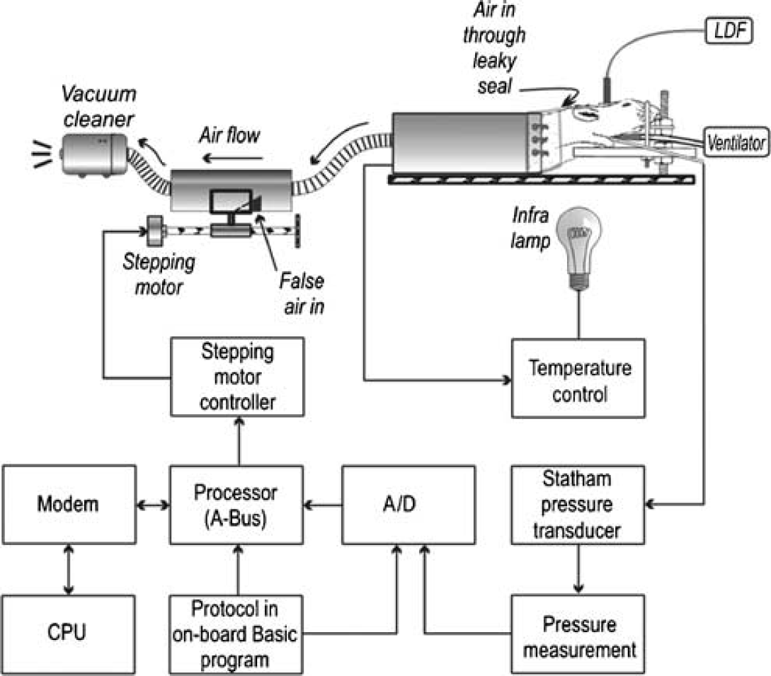
Block diagram of the experimental setup.
Blood gas parameters and hematocrit were determined in arterial blood samples withdrawn from the carotid artery (ABL 300, Radiometer, Copenhagen, The Netherlands). Corrections in blood gas parameters were made as required, in adjusting ventilation, or by intravenous administration of 4.2% bicarbonate solution. The average values before the start of laser-Doppler data collection were: pH, 7.28 ± 0.03; pO2, 98.97 ± 17.65 mm Hg; pCO2, 43.24 ± 4.4mm Hg; Sat, 95.84 ± 1.97%; Hb, 13.11 ± 1.3g/100 mL; and Hct, 40 ± 3.74%.
The animals were immobilized by Flaxèdil (SPECIA, Paris, France), and artificially ventilated (Harvard Rodent Ventilator, Model 680, Harvard Apparatus, South Matic, MA, USA). The gases were mixed and delivered to the ventilator by a calibrated flowmeter.
The core temperature was maintained (Yellow Springs Body Temperature Controller Model 73ATF, Yellow Springs, OH, USA) by controlling an infra-heating lamp at a threshold value of the rectal temperature of 37.5°C ± 0.5°C. Arterial BP was measured by a Statham pressure transducer via the catheter introduced into the carotid artery.
The Lower Body Negative Pressure Method
The lower half of the animal body was fitted in a negative pressure chamber (Dirnagl et al, 1993) (Figure 1) connected by a flexible goose-neck tubing (2.5 cm i.d.) to a vacuum cleaner providing continuous suctioning of the lower half of the body. Air was allowed to enter via a slit on the side of the tubing (‘false air’). The slit was partially covered by a stepping motor-driven sliding door, allowing fine control of airflow, and thus the degree of pooling of venous blood in the animal utilizing the arterial BP signal in a negative feedback control loop to keep BP at a preselected target value. Our system is fully programmable in that BP control is possible according to a user-defined target pressure profile.
Laser-Doppler Flowmetry
Blood cell perfusion was continuously measured by a laser-Doppler flowmeter (Model MBF3D, Moor Instruments, Millwey, Axminster, Devon, UK) in the brain cortex, through the closed calvarium made transparent by a technique adapted from Rosenblum and Zweifach (Eke et al, 1997; Rosenblum and Zweifach, 1963), as follows. The head of the animal was secured in a head holder. The scalp, subcutaneous connective tissue and the periosteum were removed. Hemostasis, if necessary, was carried out with low-intensity bipolar electrocautery (Bipolar Coagulator, Codman & Shurtleff Inc., Randolph, MA, USA) and by BoneWax (Ethicon, San Angelo, TX, USA) applied onto the exposed cranial surface. The cranium was gently thinned by a turbine dental drill (Tru-Torc II, Midwest American, IL, USA), at low r.p.m., under a high-resolution stereomicroscope at × 40 magnification until the internal compact lamina was reached. For the purpose of cleaning, cooling, and allowing for visual control, the area was repeatedly rinsed by saline of room temperature. Within the thinned area of about 4 to 5 mm in diameter, the epidural and pial vessels could be readily seen. The thickness of the bone at the site of the LDF measurement was about 160 mm, as measured by video microscopy (Eke et al, 1997). This technique fully preserved the delicate milieu of the cerebrospinal fluid space and physiological conditions of the pial and intraparenchymal circulation, which were essential requirements of this study.
The time constant of the single-pole resistor-capacitor (RC) software-implemented filter of the flowmeter was set to 0.1 secs to ensure that perfusion fluctuations are captured at the highest possible dynamics. Thus, our analysis dealt with the widest possible range of frequency components present in the signal.
Hypotensive Protocols
Steady levels of BP was maintained in steps of 100 to 80 to 60 to 40 to 60 to 80 to 100 mm Hg for 2 mins (Figure 2). A period of 30 secs was allowed for the transient between two consecutive pressure levels to occur. Before and after the down/up cycle, LDF data were collected during a period of uncontrolled BP.
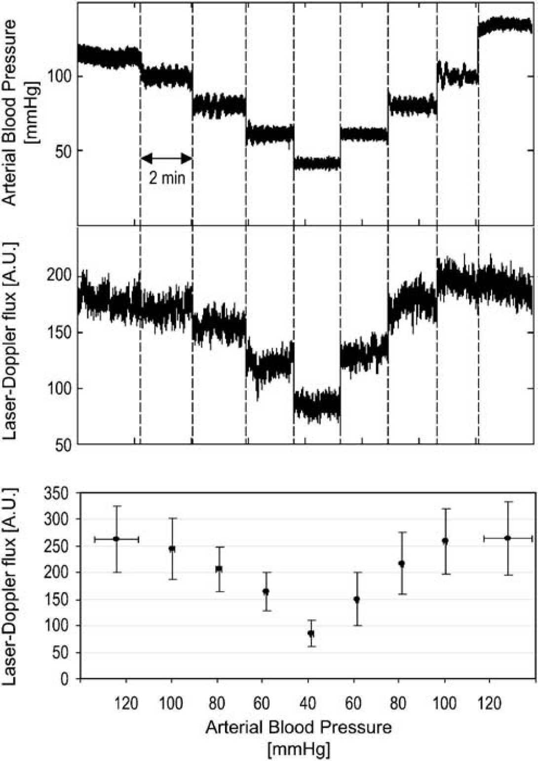
Blood pressure and laser-Doppler perfusion records for subsequent hypotensive steps from control (uncontrolled) to 40 mm Hg of mean arterial BP and returning to the control (uncontrolled) level. On the bottom panel, the results of LDF and BP statistics are seen (mean ± s.d.).
Data Acquisition, Processing, and Statistical Analysis
Signals of arterial BP and blood cell perfusion were digitized by an MP100A data acquisition system controlled by AcqKnowledge III software (BIOPAC Systems, Inc., Santa Barbara, CA, USA) at 200Hz, at 12 bits.
Arterial Blood Pressure [mmHg]
Fractal analyses were based on estimating measures of fractal self-similarity either in the time domain (Hurst exponent, H, by the bridge-detrended Scaled Windowed Variance method (bdSWV)) or in the frequency domain (spectral index, β, by a variant of the Power Spectral Density (lowPSDw,e) method). The Hurst exponent, H, is a descriptor of self-similarity of a time series. Time series exhibits self-similarity in a statistical sense in that measures, m, of fractions, φ, of series equal in distribution if properly scaled by φH. Hence, H is indeed a scaling exponent characterizing the fractal self-similarity. Its value ranges between 0 and 1. In the case of the bdSWV method, m is equivalent to standard deviation (s.d.), the standard deviation of the time series within windows of observation; whereas in case of lowPSDw,e, it is equivalent of power estimates of the Fourier spectrum within a range of frequencies. The Signal Summation Conversion method (SSC) (Eke et al, 2000, 2002) was used to classify the LDF signals as required by the bdSWV method (Eke et al, 2000, 2002).
We used numerically tested methods (Eke et al, 2000, 2002) of the Fractool software package written by the authors under Matlab 5.1 (The MathWorks, Inc., Natick, MA, USA). In addition to the methods available in the Fractool package (SSC method, a variant of the lowPSDw,e and bdSWV methods), we used the coarse-graining spectral analysis (CGSA) (Yamamoto and Hughson, 1993) to estimate the fractal content of the LDF signals. Raw-signal length varied, depending on the time available at any particular pressure step for LDF data acquisition. Fractal parameters were calculated and averaged for a set of 152 signal segments in a length of 214 data points, each shifted by 0.25 secs along the full length of the raw signal. This procedure further improved on the precision of the fractal estimates.
The largest Lyapunov exponent (Wolf et al, 1985) and the correlation dimension (Grassberger and Procaccia, 1983) as chaotic measures of complexity were calculated along with the CGSA parameter, using the TSAS software (downloadable from ftp://psas.p.u-tokyo.ac.jp/pub) run on the supercomputer of the Hungarian National Information Infrastructure Development Program. The Lyapunov exponents, λs, are dynamic measures of the nonlinear behavior of a dynamical system, which is represented in the Newtonian state space by its evolving trajectories. Over time, neighboring trajectories exponentially diverge from each other, and then, return near to their initial conditions; hence, states along the trajectories do not leave a restricted region of the state space (attractor). These dynamics along the attractor are described by the spectrum of the Lyapunov exponents. In order for a system to be qualified as chaotic, λ1 > 0 indicating divergence, λ < 0 indicating convergence, and λ3 = 0 because states oscillate on the attractor. For practical reasons, λ1, the largest Lyapunov exponent, is computed and tested for chaos. The correlation dimension, Dcorr, is a static descriptor of the chaotic attractor; in that, it determines the distance between states or phases on the well-developed attractor. For practical reasons, phases of dynamics are used, being defined as time-dependent values of a state, s, s(τ), s(2τ),…, s(nτ). The essence of the method is: to embed the dynamics into phase spaces of increasing dimension, 1 ≤ De ≤ n; and to obtain the distance, r, between all possible pairs of phase points on the attractor yielding a histogram of r showing a power law character with an exponent, ν. ν is plotted as a function of De, and Dcorr is found at the maximal (plateauing) value of n. Finding a finite correlation dimension does not necessarily imply chaos because it can also be computed for fractal signals (Osborne and Provenzale, 1989; Theiler, 1991). In order to distinguish chaotic from stochastic signals, 10 surrogate series (Theiler et al, 1992) were created from each raw series; and for each of them, the correlation dimensions and Lyapunov exponents were computed.
The mean and s.d. were calculated in Excel worksheets (Microsoft Inc., Redmond, WA, USA), and were used for the descriptive statistical characterization of the results.
Results
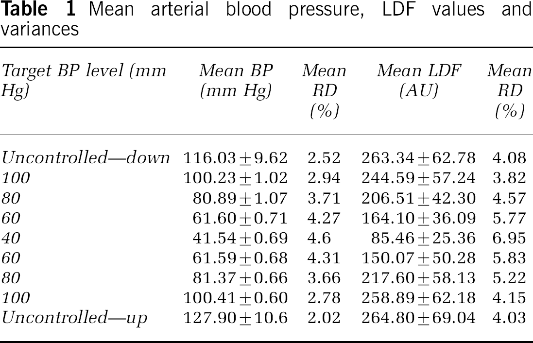
Measured values (mean ± s.d.) of mean arterial BP and blood cell flux (LDF) as they change in steps of reduced and elevated BP are shown in Figure 2 and Table 1. Target and actual values in the controlled steps from 100 to 40 mm Hg and up again to 100 mm Hg differed on average by 1.1 mm Hg only. Note that the s.d. of pressure values was a magnitude lower in controlled than that in uncontrolled states, whereas their mean relative dispersion or coefficient of variance (RD) (the mean of s.d./mean calculated for each record) increased in the downward steps, peaking at 40 mm Hg. The mean LDF value dropped during the hypotensive steps and rose to its prehypotensive, uncontrolled level, once the upward sequence of the control cycle had been completed. The mean RD of the LDF signals peaked at 40 mm Hg similarly to that of BP. The perfusion values at respective steps of the down/up control cycles did not differ (Figure 2).
Mean arterial blood pressure, LDF values and variances
At every step of BP, the fractal content of the LDF series remained high within the range of 72% to 88% (Figure 3, upper panel) and showed no dependence of the actual BP. All series proved fractional Brownian motion, which is a nonstationary fractal process (Eke et al, 2000). Their Hurst exponents as determined by the bdSWV and the lowPSDw,e methods with values of 0.29 ± 0.006 and 0.25 ± 0.012, respectively, fell in the same range, irrespective of the level of BP (Figure 3, middle panel). Their scatter around the group mean (RD) increased in response to hypotension peaking in the 40 mm Hg step (Figure 3, lower panel).
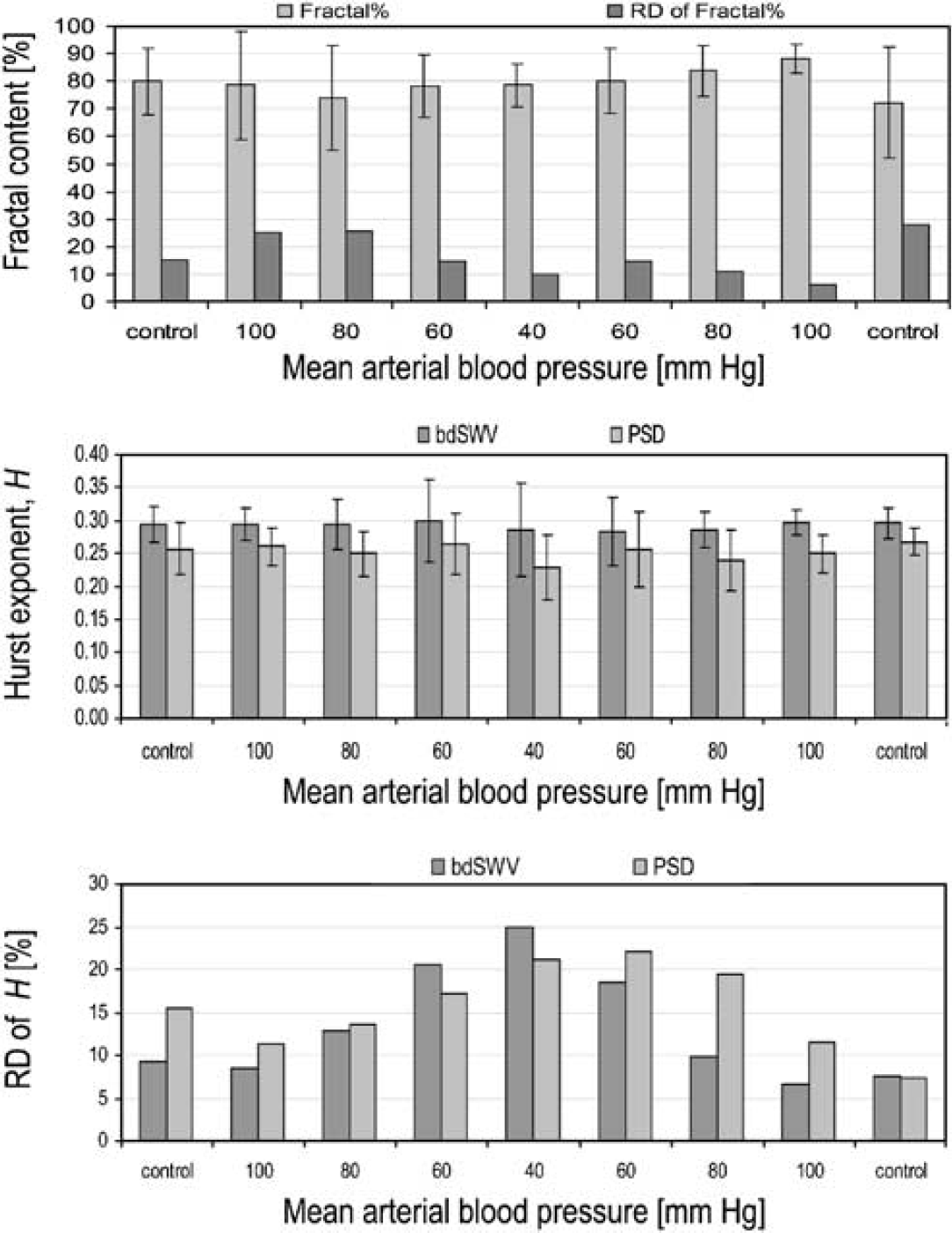
Fractal content, Hurst exponent and RD of Hurst exponent in the hypotensive steps. Mean + s.d. is shown, except for the RD.
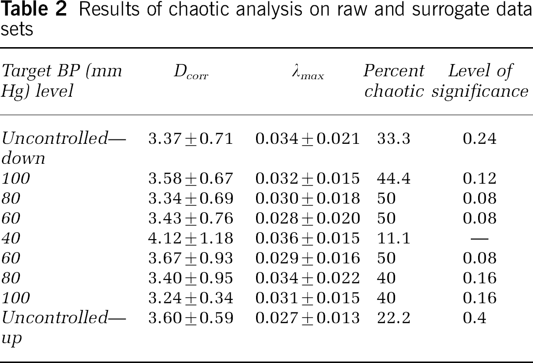
The hypotensive challenge did not alter either the correlation dimensions or the largest Lyapunov exponents (Table 2). Although their values are characteristic of a deterministically chaotic system, the outcome of their surrogate data analysis rendered some of them inconclusive in this respect (Table 2, Percent chaotic); because by postulating that the system under surrogate analysis did not contain chaotic dynamics, the null hypothesis could not be rejected. In specific terms, the tested condition of the null hypothesis was that an overlapping range of Dcorr and λmax for their respective raw and surrogate sets should indicate that the system's dynamics did not result from low-dimensional chaotic processes (Schreiber and Schmitz, 1996). The percent of such series is shown in Table 2. The level of significance at which any of these values in each hypotensive step differ from the minimal value of 11.1% obtained for the 40 mm Hg step was determined by the four-fold table method. It exhibits a minimum of 0.08 at the 80 mm Hg/down and the 60 mm Hg/down and up steps; at every other pressure level, its value in the up steps are the double of those in the downward control cycle. A value of 0.08 translates into an 8% probability that the number of chaotic series found in the respective group expressed by Percent chaotic in Table 2 differ by chance, only. This chance increases towards higher-pressure levels and is two-fold higher when pressure is raised, than that when it is lowered.
Results of chaotic analysis on raw and surrogate data sets
Discussion
The geometry of the LDF instrument's probe determines its sampling volume (Eke et al, 1997). Its diameter was 3 mm, with the source in the center and the eight detector fibers arranged in a circle around it (Eke et al, 1997). The banana-shaped volumes of photon diffusion between (Chance, 1994) the source and each of the detector fibers merged into a disk-shaped sampling volume of about 5 mm in diameter. This volume is confined within the brain cortex owing to photon diffusion properties of the brain cortex, exhibiting strong remittance and high scattering at the white matter interface that acts as a strong reflector (Eke et al, 1997), rendering the depth dimension of it to that of the brain cortex (∼2mm).
In an earlier study, we showed that the pial arterial vascular tree is a spatial fractal both in the cat (Herman et al, 2001) and in the rat (Herman, 2001). Bar (1980) reported a modular system of vascular architectonics for the rat brain cortex that bears every feature of a spatial fractal, too, which of course went unnoticed before the fractal era. This suggests that the extra- and intraparenchymal vasculature similarly undergo arborizations, according to fractal templates growing vessel segments into their volumes of supply (tissue blocks). Bar's data suggest that our sampling volume contains at least four tissue blocks of equal size, each confining one large perforating artery supplying the deep, six medium-sized perforating arteries supplying the middle, and 6 × 6 small-size perforating arteries supplying 36 of the smallest modules right underneath the pial surface. Thus, blood cell perfusion reported in this study was measured by LDF from a total of about 4 × 43, a total of 172 perforating arterial units of different dimensions.
No adverse effects of the LBNP method have been reported associated with its use in noninvasively inducing arterial hypotension (Heimann et al, 1994). A clear advantage of this method is that it does require neither invasive procedures such as hemorrhage (Barzo et al, 1993; Hudetz et al, 1992) via an arterial line, nor administration of drugs (Dirnagl and Pulsinelli, 1990), to reduce BP. In our implementation, there is a continuous airflow through the tape bandage over the surface of the lower body that could reduce the body temperature. Hence, to control it, an infrared heating lamp shielded from the site of the LDF measurement was used. The LBNP method cannot target the mean arterial BP directly, but in an indirect manner via continuously redistributing the circulating blood volume in the animal, which yields in an elevated time constant that can lead to oscillations of various amplitudes (Figure 4). As fractal analysis characterizes multi-scale patterns by fitting the data to a self-similar model either in the time or frequency domain, any particular oscillating pattern localized to a small time window or a narrow range of frequencies (Figure 4, arrows), respectively, would alter the slope of the fit to a negligible extent only.
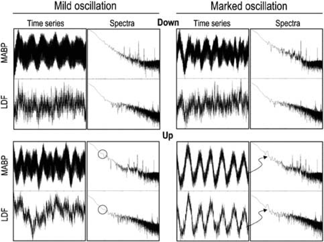
Representative examples of BP and LDF temporal records and their corresponding spectra for cases of mild and marked oscillation. Time series are for a period of 2 mins recorded during the downward and upward steps of pressure control at 60 mm Hg of MABP, Frequency range of spectra is from 0.01 to 100 Hz, displayed on a log scale. Power is shown as log|A|2 where A is the amplitude of power estimates found by FFT. Arrows indicate the frequency at which the marked oscillation can be detected in the corresponding spectra in the upward direction of control, circles show the same bands where this effect is absent in the downward direction of control. Note that the power peak at the arrow is restricted to a very narrow band of frequencies, and hence, would not alter the power slope fitted for the fractal analysis.
The traditional concept of CBF autoregulation postulates that within a certain range of perfusion pressure, the brain maintains its blood flow at the control level (Harper, 1966; Lassen, 1959). The autoregulatory range of CBF is arbitrarily defined in between lower and higher thresholds where CBF drops below 80%, or elevates above 120%, of the control value (Dirnagl and Pulsinelli, 1990; Shinohara et al, 1987). The extent to which CBF can be autoregulated depends on a number of factors such as the method of anesthesia (Hudetz et al, 1994), and the rate of BP change. Mechanisms are effective in maintaining CBF if the rate of BP change is below 0.1 mm Hg/sec (Barzo et al, 1993). In our hypotensive protocol, we chose a much higher rate (0.7 mm Hg/sec) so that the spontaneous fluctuations in LDF could be studied in the hypotensive steps without any potential interference by CBF autoregulation. As seen in Figure 2 (bottom panel), in our model and chosen protocol manifest, CBF static autoregulation is indeed avoided. With regard to the former aspect, our dose of halothane does not influence autoregulation (Dirnagl et al, 1993; Morita et al, 1977), whereas when it is given in a higher dose, it has a strong vasodilatory effect (Anderson et al, 1980).
Autoregulation is not a universal phenomenon of CBF across various species of the rat; not to the extent it has been observed in other species, like dog (Harper, 1966) or in man (Lassen, 1959): Jones et al (2002), using a hemorrhagic model, did not find autoregulation in 32% of their studied cases of Sprague–Dawley rats, the species that we used in our study; Zaharchuk et al (1999) employing the same species and model found autoregulation with a steadily declining plateau reaching the 80% level of control CBF at 50 mm Hg (with a marked scatter of data and no significance reported). As a result of rapidly declining BP and short hypotensive steps in our protocol, as expected, CBF became significantly different from control at 80 mm Hg, and also, the 80% level was reached at this level of BP; signs of an effective elimination of autoregulation, as intended. The hemorrhagic model compares well with the LBNP model in that not only BP but also cardiac output is markedly reduced. The LBNP model was originally introduced as a method of producing controlled ischemia in the brain. Nevertheless, it is suitable to be used in studies of autoregulation, such as in the work of Heimann et al (1994). In Wistar Kyoto rats anesthetized by chloral hydrate by using the LBNP model with 10-min steps, they found autoregulation with an 80% of control CBF reached at 55 mm Hg. The breakpoint on the CBF(BP) curve is relatively high at around 75 mm Hg. The data are of large scatter, with no s.d. and significance reported. In conclusion, our observed dynamics of the CBF(BP) curve fits well into those found in the same species or the same method of inducing arterial hypotension.
Fluctuations in CBF can be induced by the following three factors: BP variations; changing vascular diameters; and those emerging from the rheological properties of flowing blood. BP-induced variations in flow rate dissipate along the route from the heart to the ROI since the peak at ∼6 Hz; the typical heart rate of the rat is seen very attenuated in the LDF spectra, and except the very low frequency (VLF) range, the mean arterial blood pressure (MABP) power peaks also do get attenuated, (Figure 4). In mathematical models, rheological phenomena have been shown to be capable of producing complex microvascular temporal flow patterns (Kiani et al, 1994) due to the flow-dependent rheological behavior of blood containing a corpuscular (blood cells) and a fluid phase (plasma). This effect gains momentum with decreasing vessel diameter as postulated by the Fahraeus effect and the Fahraeus–Lindqvist phenomenon, both subject to the kinetic energy of the flowing blood.
The lack of CBF autoregulation in our hypotensive protocol does not necessarily translate into a passive behavior of the cerebral vasculature. Had this been the case, given the influence of BP shown to be dissipated above the VLF range, the only reason for which CBF fluctuations could be observed in this study would have to be of purely rheological origin. However, this could possibly not be the case, because diminishing kinetic energy of CBF concomitant with dropping BP must have resulted in diminished impact of rheology, and hence, in smaller CBF fluctuations. We found the opposite as: the variance of fluctuation amplitudes, peaking at 40 mm Hg of BP; therefore, the assumption of a passively behaving vasculature cannot hold. Consequently, what is demonstrated in this study is an actively produced CBF fluctuation (flowmotion) predominantly due to the vasomotion of many vascular segments of the arterial tree.
We report a potential coexistence of fractal and chaotic patterns in tissue perfusion, which underlines the importance of attempts separating the two. On the one hand, for this very reason, we used CGSA analysis (Yamamoto and Hughson, 1993) to determine the fractal content in the LDF signal in contrast with that of harmonics. On the other hand, we complemented our chaotic measures by those from surrogate data analysis (Theiler et al, 1992). Estimates of Dcorr and λmax suggest the presence of chaos in the fluctuations, which, in some cases, seem to get confirmed by nonoverlapping values from the surrogate data analysis (Table 2). Earlier, we found that precision of fractal estimates depends strongly on signal length (Eke et al, 2002). This kind of information is not yet available in a systematic form for the chaotic methods, that–unlike with our fractal measures-prevents us in generalizing the significance of our reported chaotic estimates.
Hypotension down to 40 mm Hg of mean arterial BP obviously presents a major challenge for the brain circulation that consequently resulted in a marked drop of perfusion in our model (Figure 2, bottom panel). This challenge, however, proved insufficient to break up the fractal correlation pattern of the LDF signals seen at control levels, in that at all pressure levels, they remained fractional Brownian motions (a nonstationary, self-similar that is fractal process (Eke et al, 2000)) with a high fractal content (Figure 3, top panel). The scatter of their Hurst exponents around means of 0.29 ± 0.006 and 0.25 ± 0.012 as measured by the bdSWV and the lowPSDw,e methods, respectively, was found increasing with lowering BP. This trend seen in the downward direction proved reversible in the upward direction of pressure control. The fact that a fractal temporal rhythm is always present in the LDF signals, although at various degrees of correlation (H) within a wide range of perfusion pressures in the brain cortex, indicates that this feature should be regarded robust and fundamental. Some of these fluctuations can be attributed to that seen in perfusion pressure (Figure 4) and some to more local mechanisms, such as flowmotion (Allegra et al, 1993) in the arterial/arteriolar tree. As seen in the MABP and LDF spectra in Figure 4, the higher the frequency power peaks in the MABP spectra, the more they get attenuated in the corresponding range of frequencies in the LDF spectra. The low-frequency power peaks remain present in isolated form in both spectra (lower right panels in Figure 4). Flowmotion seems to operate at the local (segmental) level, according to the rules of nonlinear control, whereas from these local dynamics, the regional pattern appears to be assembled across multiple spatial and temporal scales, according to the rules of self-organizing (Turcotte et al, 2002; Waliszewski, 2005), self-similar systems lending to cerebro-cortical perfusion a robust temporal dynamics.
In contrast with the traditional trends of experimentation using in situ or ex vivo models and making statistically representative measurements at critical time points in response to a perturbation, our approach leaves the object of study intact and captures in a high definition temporal record, the full spectrum of the dynamics of the physiological system (regional blood cell perfusion) under observation. Our holistic analysis focused on temporal structuring is the one that offers insight into the nature of CBF by exploring if the spontaneous CBF fluctuation seen in these records is indeed disordered (cannot result from control), or follows some specific order in time, which must be the result of control of some sort. In conclusion, our study produces additional insight into the nature of CBF in that it shows that individual temporal events in CBF are fractally correlated as blood flows through the brain cortex. We have also shown that the degree of this special correlation, known as fractal order, remains present even under severely reduced perfusion of the brain, grossly being independent of BP. Our results suggest that a likely candidate of control behind the fractal dynamics is self-organization (Turcotte et al, 2002; Waliszewski, 2005), rather than the activity of some control center or a few controlling factors for our chaotic analysis could not equivocally demonstrate the presence of the latter.
A combination of the following three elements in our approach offers a future potential in ischemia and stroke research. Firstly, the LBNP method—originally introduced as a noninvasive technique to produce global cerebral ischemia (Dirnagl et al, 1993) in a controlled manner—with our improvements is indeed a reliable tool to establish various ischemia protocols. Most currently used ischemia models operate by permanently occluding the arterial supplies of the brain, whereas this model also allows for a finely adjustable ischemic insult that can be followed by reperfusion. Secondly, continuous optical measurement of cerebral perfusion, such as by LDF, provides high definition time series, of all perfusion events occurring simultaneously within the ROI in the course of ischemia. Thirdly, our fractal tools stepping beyond computing measures of descriptive statistics can explore from these time series the temporal structuring of flow events underlying the observed flowmotion in the form of frequency distribution of spectral estimates. Under normal conditions, this distribution is wide and follows an inverse power law relationship, typical of temporal fractals. This wide spreading of power across frequencies is produced by the vasomotion of generations of vascular segments along the arterial tree, each of them contributing at their intrinsic frequency with increasing power towards the low frequencies. In addition, the degree of synchrony is diminishing towards more distal segments of the arterial tree (Yipintsoi et al, 1973). It is known that ischemia in the brain invokes vasodilation (O'Regan, 2005; Tomita et al, 1980) that appears to be mediated by various factors; among them, most likely, adenosine (O'Regan, 2005). In long-term ischemia, a marked decrease in blood volume due to collapse of vessels or their compression by edema is likely to occur. In either case, our approach can identify that these pathological deviations in the vascular caliber do occur, by detecting a deviation of power slope from that of fractal structuring of flowmotion characteristic of the normal conditions that follows an inverse power law across the spectrum. In fact, such alterations in the spectra may not only occur due to ischemia, but also as a result of age-related stiffening of small arterial segments of the cerebral vasculature, as was demonstrated most recently using near-infrared monitoring of cerebral blood volume fluctuations in humans (Eke et al, 2005). Our fractal analysis of high definition perfusion records obtained in computer-controlled ischemia models therefore can be instrumental in monitoring and understanding the dynamics of how fractally correlated vasomotion-induced flowmotion—a phenomenon linked with normal functioning of cerebral vasculature—breaks up as a result of an emerging loss of vasomotion activity, most likely starting with the most distal segments of the arterial tree.
Footnotes
Acknowledgements
The computer program ‘Fractool’ running on the Macintosh, PC, and Unix platforms for estimating the Hurst exponent of physiological time series are available on the Web at http://www.elet2.sote.hu/eke/FRACTPHYS/. This program can be freely distributed as long as the ‘readme’ file is included and the use of the program is properly acknowledged. Other fractal programs are available at ![]() , thanks to Mr Gary Raymond. The authors thank Professor Peter Sandor for lending his LDF monitor. The authors greatly appreciate the valuable discussions with Dr Laszlo Kocsis.
, thanks to Mr Gary Raymond. The authors thank Professor Peter Sandor for lending his LDF monitor. The authors greatly appreciate the valuable discussions with Dr Laszlo Kocsis.