Sage Journals: Discover world-class research

Abstract

Estimates of cerebral blood volume (CBV) obtained from dynamic contrast T2* -weighted magnetic resonance imaging (MRI) tend to be significantly higher than values obtained by other methods. This may relate to the common assumption that the proportionality constants relating signal change to contrast concentration are equal in tissue and artery. To test this hypothesis and provide estimates for the ratio of those proportionality constants, the authors compared measurements of CBV by both MRI and computed tomography (CT) scans in nine healthy volunteers obtained using identical kinetic paradigms for the two imaging modalities. Both boluses and infusions of contrast were studied. Measurements were made in nine anatomic regions of interest of the cerebral hemispheres bilaterally. Cerebral blood volume values obtained by CT were generally lower than those obtained by MRI, especially in the cerebral cortex. As a result, the calculated values of the ratios of proportionality constants relating signal change to concentration in tissue and artery after bolus injections were significantly less than 1 in cortex (0.69) and white matter (0.76), although not in deep gray matter structures (0.87). Values of the ratios based on infusion measurements were closer to 1. In addition, CBV measurement errors with bolus MRI were significantly larger than those observed with infusion MRI or by CT. The reasons that the constants differ from 1 and for the larger variance of bolus MRI are discussed in terms of the T2* signal mechanisms. These studies help define the magnitude by which CBV is overestimated with typical T2*-weighted perfusion imaging. Infusion measurements of CBV can reduce the variance intrinsic to T2* MRI and lessen the likelihood of type II error.

Keywords

CBF CBV CT MRI perfusion

Introduction

Maps of relative cerebral blood volume (CBV) by dynamic contrast T2*-weighted magnetic resonance imaging (MRI) are commonly created during clinical assessment of patients, but quantification of CBV by MRI remains a challenging goal, with values of CBV that are frequently overestimated compared with other imaging methods. Magnetic resonance imaging estimates of CBV usually involve measurement of the area under the curve (AUC) of the amplitude of the arterial and tissue signal changes resulting from an intravenous bolus injection of gadolinium (Gd) (Smith et al, 2000). Our laboratory employs an alternative but related approach using measurements of stable artery to tissue ratios of signal change during rapid infusions of Gd (Tudorica et al, 2002; Newman et al, 2003).

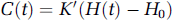
It has been observed empirically that plasma Gd concentrations can be estimated based on change in relaxivity (Weisskoff et al, 1994), using the equation:

C (t) = K Δ R 2^{*} (t) = - K \ln (S (t) / S_{0}) / T E

(1)

where C(t) is the concentration of Gd in the artery or tissue, K is a proportionality constant, ΔR2*(t) is the relaxation rate change at any time, S(t) is the instantaneous signal, S₀ is the signal before contrast arrival and TE is echo time. By analogy, it is commonly assumed that a similar relationship can be applied to the arterial input function (AIF), although several studies suggest that a quadratic relationship is more appropriate for whole blood (Akbudak et al, 1998; van Osch et al, 2003). As K depends on numerous factors, including magnetic field strength, local inhomogeneities, the specific pulse sequence and tissue properties such as anisotropic flow orientation and velocity (Boxerman et al, 1995), its value cannot be calculated easily from physical principles. As a result, most estimates of CBV are obtained by applying equation (1) to tissue and artery, taking the ratio of the integrated signal change in tissue to that in artery and assuming that the individual values of K_tis, relating signal change to concentration in tissue, and K_art, relating signal change to concentration in an artery, are equal to one another. The purpose of the present study was to test the assumption that the ratio, K_tis/K_art, is equal to 1.

Quantification of CBV by dynamic contrast CT scanning does not have this disadvantage since signal change in Hounsfield units under conditions typically employed in humans is linearly related to contrast concentration and the relationship

C (t) = K^{'} (H (t) - H_{0})

(2)

is not dependent on flow orientation, velocity or acquisition sequence, unlike MRI (Hammer et al, 1995; Nosil et al, 1989). The simplicity of this relationship, which applies equally in tissue and artery so that the relationship K_tis = K_art actually does apply, provides the basis of the present experiments. By using identical kinetic paradigms to compare the ratio of signal change in tissue and artery obtained by MRI to the ratio of signal change in tissue and artery obtained by CT, it is possible to obtain an experimental estimate of the ratio, K_tis/K_art for MRI. If the estimates for this ratio are less than 1, then this may help to explain the overestimation of CBV routinely obtained by T2*-weighted MRI.

Theory

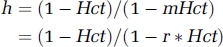
Most dynamic contrast measurements of CBV use a bolus injection of contrast and integration of concentration over time in tissue and artery:

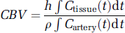
C B V = \frac{h \int C_{t i s s u e} (t) d t}{ρ \int C_{a r t e r y} (t) d t}

(3)

where

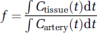
f = \frac{\int C_{t i s s u e} (t) d t}{\int C_{a r t e r y} (t) d t}

(4)

is the tissue plasma volume fraction and the concentrations specifically refer to the plasma concentrations of the contrast agent, ρ is the density of brain tissue, set to 1.04 g/ml (Axel, 1980), and h corrects for the fact that the hematocrit in large vessels is greater than the hematocrit in small vessels. The value of h can be calculated from the measured venous hematocrit using

\begin{aligned} h = & (1 - H c t) / (1 - m H c t) \\ = & (1 - H c t) / (1 - r * H c t) \end{aligned}

(5)

where Hct and mHct are the large vessel and microvessel hematocrits, respectively, and r = mHct/Hct. It is common to assume that r can be represented by a single constant value throughout the brain. For this study, a value of 0.85 was assigned to r based on PET data in humans (Phelps et al, 1979).

Explicitly introducing the relationship for MRI between signal change and concentration from equation (1) into equation (3) yields

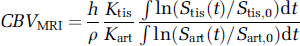
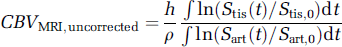
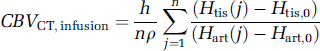
C B V_{M R I} = \frac{h}{ρ} \frac{K_{t i s}}{K_{a r t}} \frac{\int \ln (S_{t i s} (t) / S_{t i s, 0}) d t}{\int \ln (S_{a r t} (t) / S_{a r t, 0}) d t}

(6)

Practical application of equation (6) involves integration of the AUC for amplitude of signal change in tissue and artery, either nonparametrically by simple numerical integration, parametrically after curve fitting with a gamma variate or related function, or by an alternative method (Perkio et al, 2002). To the best of our knowledge, all studies to this point also apply the assumption that K_tis/K_art = 1. For the sake of future notation, we define this uncorrected MRI estimate of CBV as

C B V_{M R I, u n c o r r e c t e d} = \frac{h}{ρ} \frac{\int \ln (S_{t i s} (t) / S_{t i s, 0}) d t}{\int \ln (S_{a r t} (t) / S_{a r t, 0}) d t}

(6a)

The equation for CBV by CT scan, based on equations (2) and (3), and making use of the equivalent relationships between signal change and concentration in tissue and artery for CT, is entirely analogous

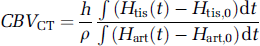
C B V_{C T} = \frac{h}{ρ} \frac{\int (H_{t i s} (t) - H_{t i s, 0}) d t}{\int (H_{a r t} (t) - H_{a r t, 0}) d t}

(7)

As for MRI, application of this equation requires an integration of signal change over time.

An analogous equation to Equation (6a) can be derived for measuring CBV by MRI infusion (Newman, 2003):

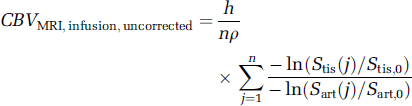
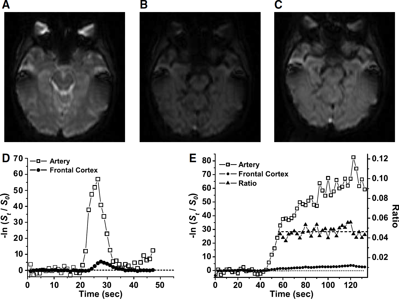
\begin{aligned} C B V_{M R I, i n f u s i o n, u n c o r r e c t e d} = & \frac{h}{n ρ} \\ \times \sum_{j = 1}^{n} \frac{- \ln (S_{t i s} (j) / S_{t i s, 0})}{- \ln (S_{a r t} (j) / S_{a r t, 0})} \end{aligned}

(8)

where n is the number of ratios measured within the portion of the infusion during which the ratio is stable, S_tis(j) and S_art(j) are the jth signal measurements during that stable portion in the tissue region of interest (ROI) and artery, respectively, and S_{tis, O} and S_{tis, O} are the average signals in tissue and artery during the baseline period before arrival of contrast. Note that the ratio of signal change in tissue to that in artery is stable even though the individual curves have not reached steady state (Newman, 2003; Figure 1E).

Figure 1

Magnetic resonance composite: (A) precontrast, (B) bolus at peak, (C) infusion at max, (D) time course of bolus for MCA and frontal cortex, (E) time course of infusion for MCA and frontal cortex with the ratio of signal change in tissue to that in artery plotted against the right-hand Y-axis. The mean ratio in (E) is indicated by the dashed line and zero signal change is indicated by the dotted line.

Similarly, measurement of CBV by CT infusion can be written as

C B V_{C T, i n f u s i o n} = \frac{h}{n ρ} \sum_{j = 1}^{n} \frac{(H_{t i s} (j) - H_{t i s, 0})}{(H_{a r t} (j) - H_{a r t, 0})}

(9)

Since the actual CBV must be the same whether measured by CT or MRI, assuming that both CT and MRI contrast agents are restricted to plasma, it follows that, for bolus measurements:

\begin{aligned} C B V_{C T} = & C B V_{M R I} \\ = & (K_{t i s} / K_{a r t}) C B V_{M R I, u n c o r r e c t e d} \end{aligned}

(10)

(K_{t i s} / K_{a r t}) = C B V_{C T} / C B V_{M R I, u n c o r r e c t e d}

(10a)

Note that the values of h and ρ cancel analytically. The relationship in equation (10a) applies whether CBV is obtained from bolus data with measurement of AUC nonparametrically or parametrically or from infusion data, as long as the same kinetic paradigm is used for CT and MRI. In general, the value of (K_tis/K_art) may differ as a function of either the kinetic paradigm used or the brain region studied.

Materials and methods

Subjects and Acquisitions

All protocols were approved by the University of Wisconsin Institutional Review Board for research on human subjects. Ten healthy subjects, free of any acute or chronic disease, were recruited from among the staff and students associated with the medical center. At 1 day before the study, a blood sample was taken for assay of creatinine. For the imaging session, each subject had a 20-gauge intravenous needle inserted into the ante-cubital vein by a qualified nurse with simultaneous blood sampling for determination of hematocrit. Four of the 10 subjects were women. The mean age was 35.5 years, with a range of 20 to 47 years.

For all subjects MRI preceded CT imaging to avoid exposing subjects to the risk of CT contrast before learning that they could not complete the MRI due to claustrophobia. For both modalities, the bolus scan preceded the infusion. This fixed sequence was chosen to maximize experimental consistency because prior studies in our laboratory have shown no effect of the sequence on CBV measurements. CT imaging was performed within 1 h of MRI for all subjects.

All MR images were acquired on a GE Sigma 1.5 T MRI with echo planar capability using a standard human head RF coil (General Electric Medical Systems, Milwaukee, WI, USA). Each subject's imaging session included an anatomic reference scan and two perfusion acquisitions, bolus and infusion, using the same set of 12 5-mm slices (1-mm gap), which was oriented obliquely with the third slice parallel to the inferior surface of the medial frontal lobe to minimize susceptibility artifact in the region of the middle cerebral artery (MCA) (Figures 1A to 1C). All perfusion scans were acquired as multiple blocks of single-shot echo planar images with a 22-cm field of view (FOV) and 128 × 64 acquisition matrix, reconstructed to 128 × 128. The anatomic scan was a T1-weighted FLAIR (TR 2200/TE 7.6/TI 750 ms, 2 averages) with a 22-cm FOV and 256 × 256 matrix. The bolus perfusion acquisition had a TR of 1150 ms, TE of 35 ms, and 90° flip angle. The infusion perfusion acquisition had a TR of 2500 ms and the same TE and flip angle. All perfusion sequences were timed so that at least 10 images were obtained before contrast arrival to ensure an accurate baseline signal value. For the bolus acquisition, 70 μmol/kg of gadodiamide (Omniscan®, Nycomed, NY, USA) was delivered over 3 secs (but not exceeding 4 mL/sec), using an MR-compatible injector (Medrad, Inc., Indianola, PA, USA). For the infusion, 180 μmol/kg of contrast was diluted to 90 mL with normal saline and then infused over 90 secs at 1 mL/sec, producing an infusion rate of 2 μmol/kg/sec. The total Gd dose for the bolus and infusion pair was thus 250 μmol/kg.

All computerized tomography perfusion (CTP) images were acquired on a GE Lightspeed 8- or 16-slice detector scanner (General Electric Medical Systems, Milwaukee, WI, USA). Each subject imaging session included anatomic reference scans and two perfusion acquisitions: bolus and infusion. Both scans utilized the same four-slice set (5 mm thickness with no gap, axial orientation). The bolus scan was acquired over 40 repeats with no interscan delay and was initiated at the start of the bolus injection. The infusion scan utilized a 1-sec interscan delay to increase the duration of the scan to 80 secs and was initiated 10 secs before the start of the infusion to increase the number of baseline frames. All perfusion scans localized the region of the MCA on the lowest slice for continuity (Figures 2A to 2C). All perfusion sequences were timed so that at least eight images were acquired before contrast enhancement for a baseline analysis. For the bolus scan, 50 cm³ of Omnipaque Iohexol (300 mg/mL; Princeton, NJ, USA) with a 30-cm³ saline chase, both at 5 mL/sec, was delivered using a Medrad power injector (Medrad, Inc., Indianola, PA, USA). For the infusion scan, 50 cm³ of Omnipaque Iohexol (300 mg/mL) with a 30-cm³ saline chase was delivered using the Medrad power injector at 1 mL/sec for 50 secs. The total dose of iodinated contrast for both perfusion scans was 100 cm³.

Figure 2

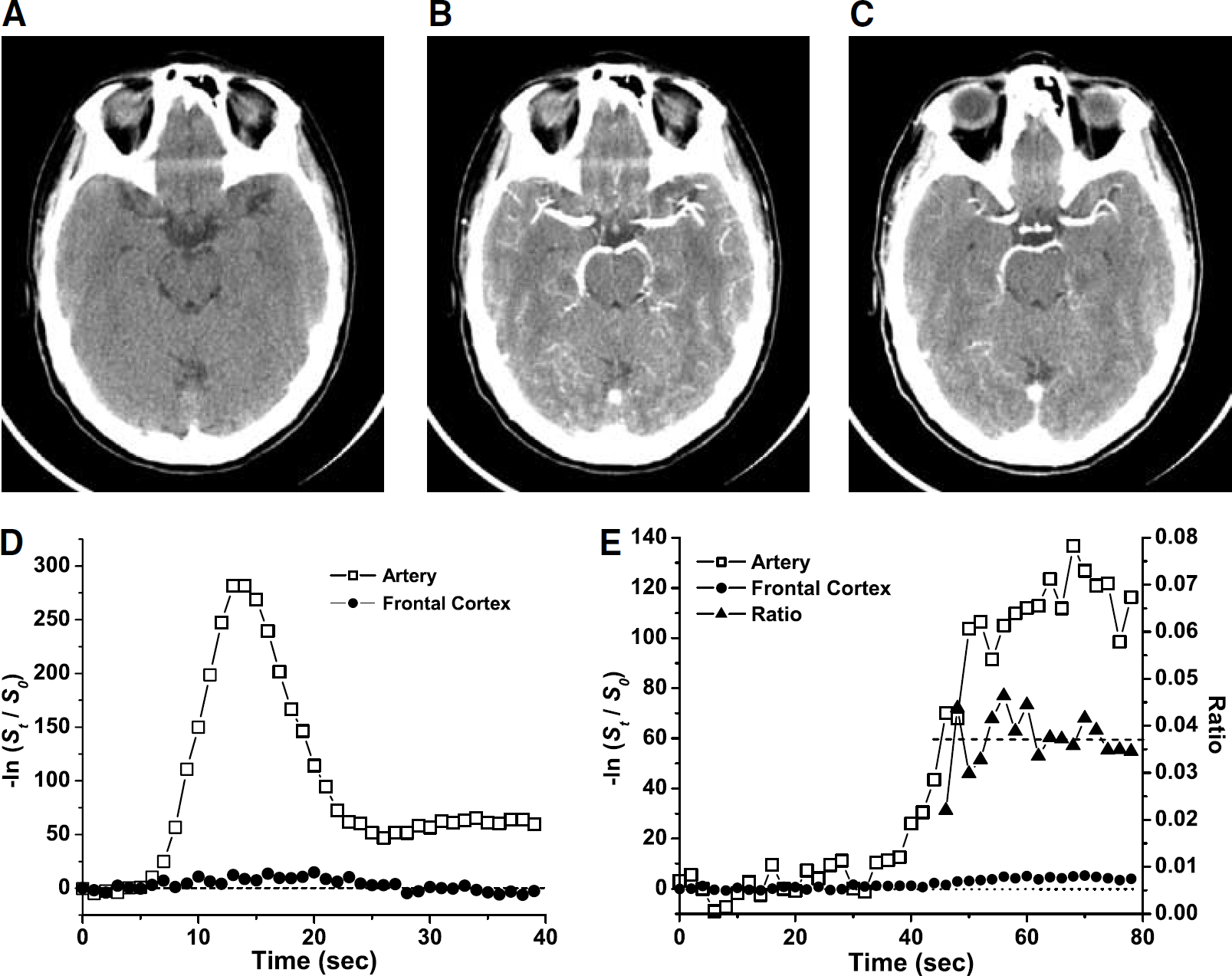
Computed tomography composite: (A) precontrast, (B) bolus at peak, (C) infusion at max, (D) time course of bolus for MCA and frontal cortex, (E) time course of infusion for MCA and frontal cortex with the ratio of signal change in tissue to that in artery plotted against the right-hand Y-axis. The mean ratio in (E) is indicated by the dashed line and zero signal change is indicated by the dotted line. Figures 1E and 2E are for the same region of frontal cortex from the same subject and are directly comparable.

Image Analysis

All perfusion data were analyzed using custom software written in MatLab (Mathworks, Inc. Natick, MA, USA). Regions of interest were drawn to conform with anatomic brain structures (Figure 3). For MRI, ROIs were drawn on the magnified first image of the perfusion scan, while simultaneously visualizing the equivalent slice of the reference anatomic scan at the same magnification. For CT, ROIs were drawn directly on the magnified first image of the perfusion sequence. Vascular ROIs were drawn for the MCA and posterior cerebral artery (PCA) bilaterally, and for the straight sinus (SS). Arterial ROIs were drawn approximately 1 cm distal to the origin of the vessel to minimize venous contamination. Bilateral tissue ROIs were drawn and grouped as follows: (1)

Cortical gray matter–-lateral superior frontal (FC), lateral posterior temporal (TC), occipital pole (OC).

(2)

Deep gray matter–-caudate (CD), globus pallidus (GP), putamen (PUT), thalamus (TL).

(3)

White matter–-anterior frontal white matter (AF), optic radiations (OR).

Figure 3

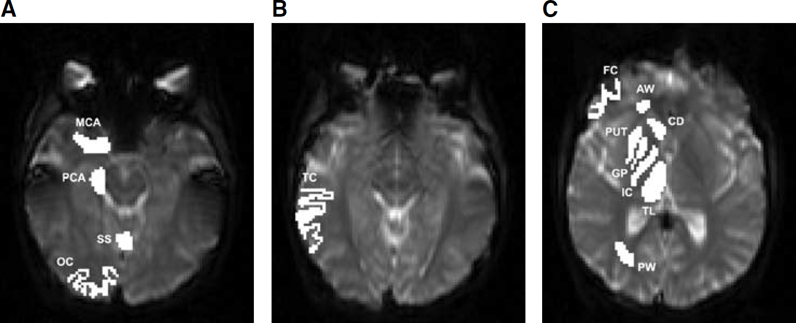
Regions of interest used in study, shown for one side only.

For the cortical ROIs, care was taken to exclude at least one pixel for MRI and four pixels for CT at the boundary of the cortical surface to reduce vascular contamination.

Pixel selection procedures for vascular structures and tissue ROIs from MRI have been described in detail previously (Newman et al, 2003). Pixels for vascular ROIs were selected visually from the signal versus time curve based on early arrival time, large amplitude (but avoiding signal values below 10), and narrow half-width. The same procedures were followed for CT data.

Baseline signal values were obtained by averaging signal for the frames in each ROI before arrival of contrast. For MRI, the first two frames were always excluded from baseline calculations to avoid effects due to unsaturation, so that 8 to 10 frames were included, depending on the earliest contrast arrival time in either MCA. For CT, baseline was calculated from the first frame and included six to eight frames.

Relative concentration for each pixel was calculated using equation (1) for MRI and equation (2) for CT. For either modality, a concentration-time curve was created for each ROI in each hemisphere of each subject by calculating the mean of the relative concentration for all selected pixels at each time point (Figures 1D to 1E and 2D to 2E). Cerebral blood volume was calculated from these averaged kinetic curves.

Nonparametric area under the curve (npAUC) was calculated for MRI or CT data by summing the relative signal change from the first frame after baseline to the last frame of the acquisition multiplied by the time interval. Parametric area under the curve (pAUC) was obtained by fitting the arterial concentration-time curves to a gamma variate function and the tissue concentration-time curve to a five-parameter lagged normal density function (Knudsen et al, 1994) by nonlinear least-squares analysis using the simplex method within MatLab. Before subjecting data to the nonlinear fitting routines, the data curves were interpolated using the MatLab INTERP subroutine to increase the number of points on the concentration-time curves fivefold.

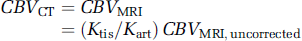
Cerebral blood volume was calculated from AUC measurements using equation (6a) for MRI and equation (7) for CT. Cerebral blood volume was calculated from infusion data using equation (8) for MRI and equation (9) for CT. In either case, this involved visually identifying the stable portion of the arterial curve and then averaging the ratio of signal change in tissue to signal change in artery over all frames within the stable portion of the curve, typically approximately 20 frames (Newman et al, 2003). Note that, as a result of using equations (6a) and (8) for MRI, all values of CBV presented for MRI are uncorrected values.

Values of K_tis/K_art were calculated for all three methods of analysis (npAUC, pAUC, or infusion) using equation (10a) for each ROI in each hemisphere of each subject before averaging. Gray matter/white matter ratios were calculated for each subject by taking the mean of all cortical and deep gray matter ROIs and then dividing by the mean of the subject's white matter ROIs.

Contrast to noise was calculated for bolus concentration-time curves by dividing the maximum height of the curve by the standard deviation of the baseline.

Statistics

Means and standard deviations were calculated by averaging the right and left ROI for each individual, calculating values of CBV, (K_tis/K_art), gray/white ratios, and contrast to noise ratios (CNR) for all ROIs and tissue types for each individual, and then averaging among all individuals to obtain the reported values. Comparisons were performed by paired t-tests and reported without correction for the number of comparisons. Comparisons of ratios were performed on log transforms of the data.

Cerebral blood volume measurement errors were analyzed statistically. To simplify the analysis, the comparison was restricted to npAUC and infusion data. Thus, variance was compared for four methods, two CT and two MRI, for sets of data from cortex, deep gray, and white matter in the nine subjects. The percent deviation from the median and the absolute value of that percent deviation was calculated for each tissue type of each subject by each method. Results were then compared using both two-way analysis of variance (ANOVA) of the data and permutation analysis. This latter statistic properly accounts for correlations that may arise from the repeated measures made on the same subject in a manner that two-way ANOVA does not.

Results

Cerebral blood volume values for the nine ROIs are shown for all methods in Table 1. Cerebral blood volume values obtained from CT data are uniformly at or below 0.032 mL/g, and lower than those for MRI for all ROI by all methods. For both CT and MRI, mean values tend to cluster into groups. For CT, gray matter values appear larger than white matter values. For MRI, all three tissue types appear to differ, in the sequence cortex > deep gray > white matter. Also, for MRI, the standard deviation of the means appears lower for CBV measurements by infusion.

Table 1

CBV values by ROI and method

ROI	CT			MRI

	npAUC	pAUC	Infusion	npAUC	pAUC	Infusion
FC	0.024 ± 0.005	0.026 ± 0.009	0.027 ± 0.005	0.035 ± 0.010	0.041 ± 0.010	0.034 ± 0.005
OC	0.024 ± 0.005	0.026 ± 0.006	0.031 ± 0.006	0.041 ± 0.018	0.048 ± 0.020	0.044 ± 0.006
TC	0.021 ± 0.005	0.023 ± 0.005	0.027 ± 0.006	0.035 ± 0.012	0.040 ± 0.013	0.035 ± 0.008
CD	0.026 ± 0.007	0.028 ± 0.008	0.028 ± 0.004	0.029 ± 0.011	0.033 ± 0.012	0.029 ± 0.004
GP	0.022 ± 0.005	0.023 ± 0.006	0.026 ± 0.005	0.030 ± 0.010	0.033 ± 0.010	0.028 ± 0.004
PUT	0.027 ± 0.005	0.029 ± 0.005	0.032 ± 0.005	0.034 ± 0.012	0.038 ± 0.014	0.032 ± 0.005
TL	0.024 ± 0.006	0.026 ± 0.006	0.029 ± 0.005	0.035 ± 0.013	0.040 ± 0.014	0.034 ± 0.005
AF	0.020 ± 0.007	0.023 ± 0.008	0.022 ± 0.005	0.032 ± 0.014	0.035 ± 0.016	0.032 ± 0.014
OR	0.016 ± 0.003	0.018 ± 0.003	0.021 ± 0.005	0.025 ± 0.004	0.030 ± 0.013	0.025 ± 0.004

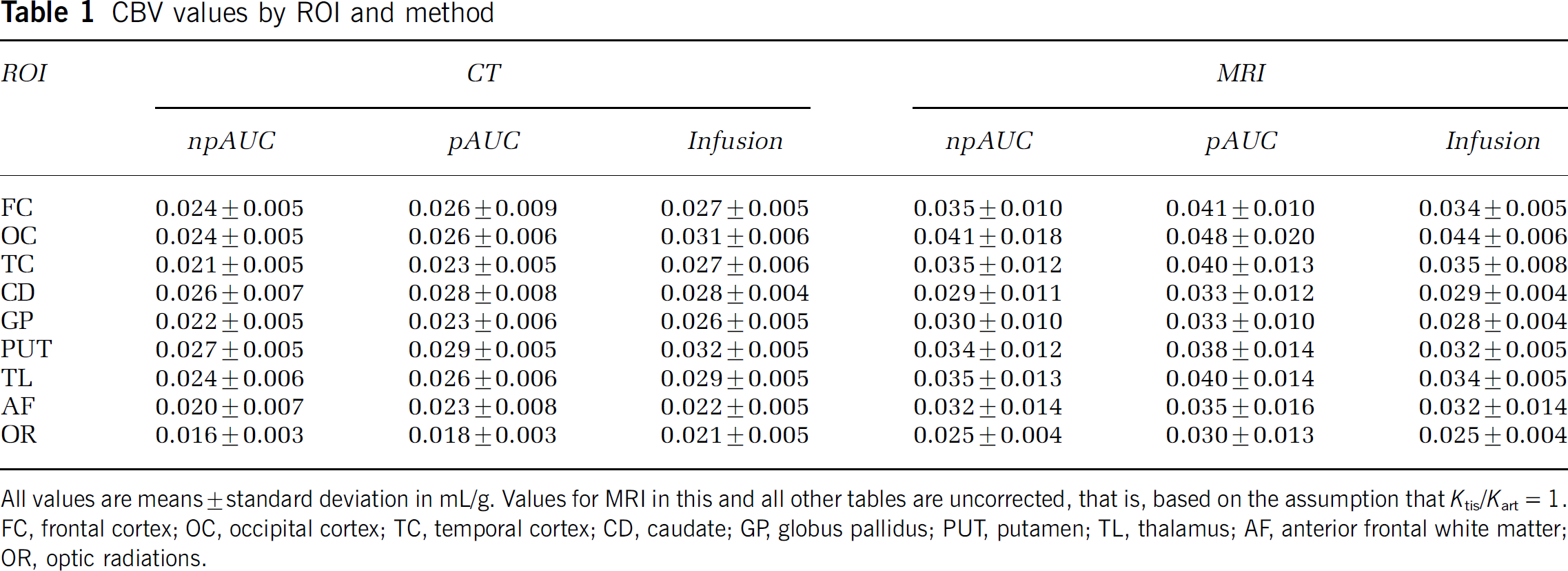
All values are means ± standard deviation in mL/g. Values for MRI in this and all other tables are uncorrected, that is, based on the assumption that K_tis/K_art= 1. FC, frontal cortex; OC, occipital cortex; TC, temporal cortex; CD, caudate; GP, globus pallidus; PUT, putamen; TL, thalamus; AF, anterior frontal white matter; OR, optic radiations.

These patterns are more apparent when the data are analyzed by tissue type (Table 2). All three CT methods appear to give similar results although values by infusion appear slightly larger. Pairwise comparisons of the CT data, however, reveal only a marginally significant difference in cortex between infusion and npAUC values (P = 0.026). Owing to the very tight correlation between npAUC and pAUC, even the small differences between them are statistically significant (P < 0.01). Pairwise comparisons between tissue types for CT data reveal significant differences between white matter and both gray matter regions (P < 0.001), but no difference between cortical and deep gray matter with any of the three methods. Bolus MRI data show consistently larger variance.

Table 2

CBV Values by tissue type and method

Method	Cortex	Deep gray	White
CBV by CT
npAUC	0.023 ± 0.004	0.025 ± 0.005	0.018 ± 0.004
pAUC	0.025 ± 0.005	0.026 ± 0.005	0.020 ± 0.004
Infusion	0.028 ± 0.004	0.029 ± 0.004	0.022 ± 0.005
CBV by MRI
npAUC	0.037 ± 0.012	0.032 ± 0.011	0.030 ± 0.012
pAUC	0.043 ± 0.013	0.036 ± 0.012	0.032 ± 0.014
Infusion	0.038 ± 0.005	0.031 ± 0.004	0.026 ± 0.003

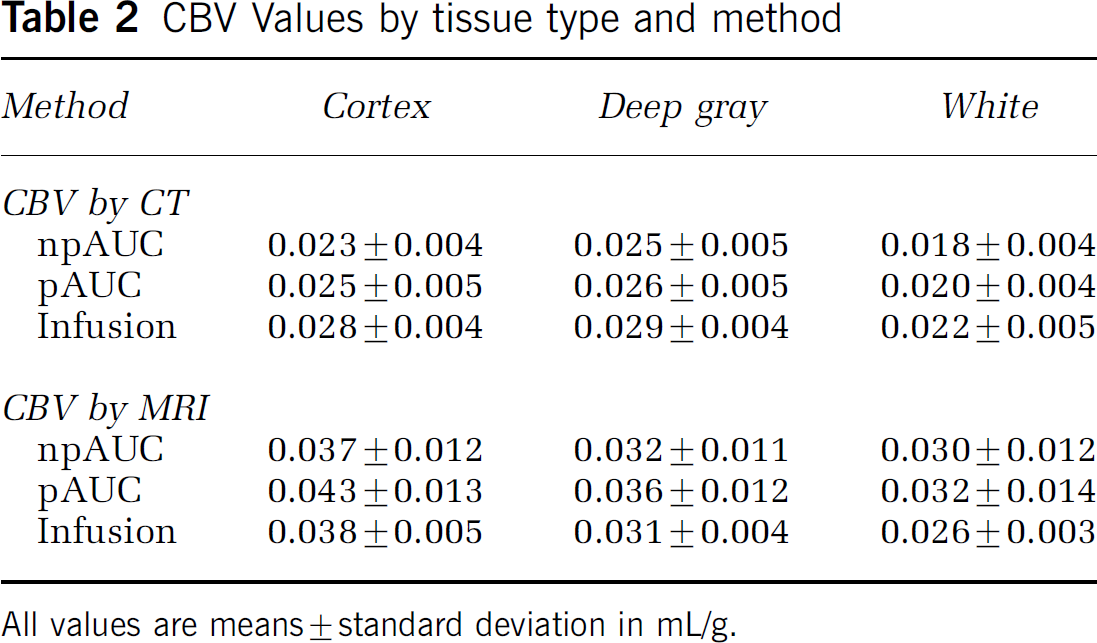
All values are means ± standard deviation in mL/g.

Uncorrected CBV values obtained by MRI are generally higher than values by CT, although only the cortical values differ significantly between the two imaging techniques (P < 0.01 for npAUC, P < 0.005 for pAUC and infusion). The three analytical approaches to MRI produce similar results except for marginal differences between npAUC and pAUC (P < 0.05). Cortical CBV differ from deep gray and white matter CBV by all three analytical methods (P < 0.005). The difference between deep gray and white matter is significantly different, however, only when using infusion data (P = 0.011).

Differences in CBV measurement errors among the CT and MRI methods are readily apparent from inspection of Figure 4, where the values for each tissue type of each individual are presented graphically. The systematic differences in CBV between CT and MRI discussed above are apparent in the graphs of column 1 of the figure. The percent deviation from the median for each tissue type of each method is shown in column 2 and the absolute percent deviations are shown in column 3. Table 3 summarizes the observed measurement variations, where each value is a summary of the individual values made over the nine subjects. Two-way ANOVA of the data in Table 3 shows significant differences between methods (P = 0.012), but not between tissue types (P = 0.21). Statistical differences between methods are also shown by permutation analysis (P = 0.006). The least variability occurs with infusion MRI.

Figure 4

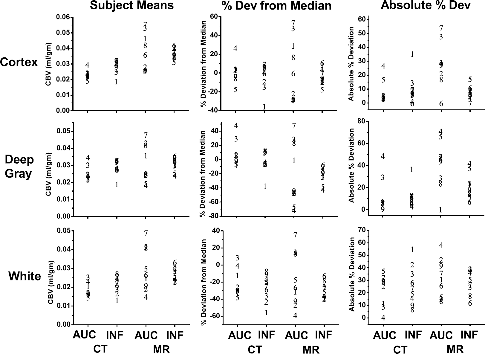
Cerebral blood volume results for CT and MR, bolus, and infusion for each subject (represented by #) by tissue type in the first column, the % deviation from the median in the second column, and the absolute % deviation from the median in the third column.

Table 3

Median absolute percent deviations from median of CBV values

Method	Cortex	Gray	White
CT npAUC	10.82	10.41	22
CT infusion	8.37	19.9	14.48
MR npAUC	21.5	51.27	43.32
MR Infusion	8.23	7.23	7.91

Values represent the mean among all nine subjects of the absolute value of percent deviations from the median for each tissue type and method.

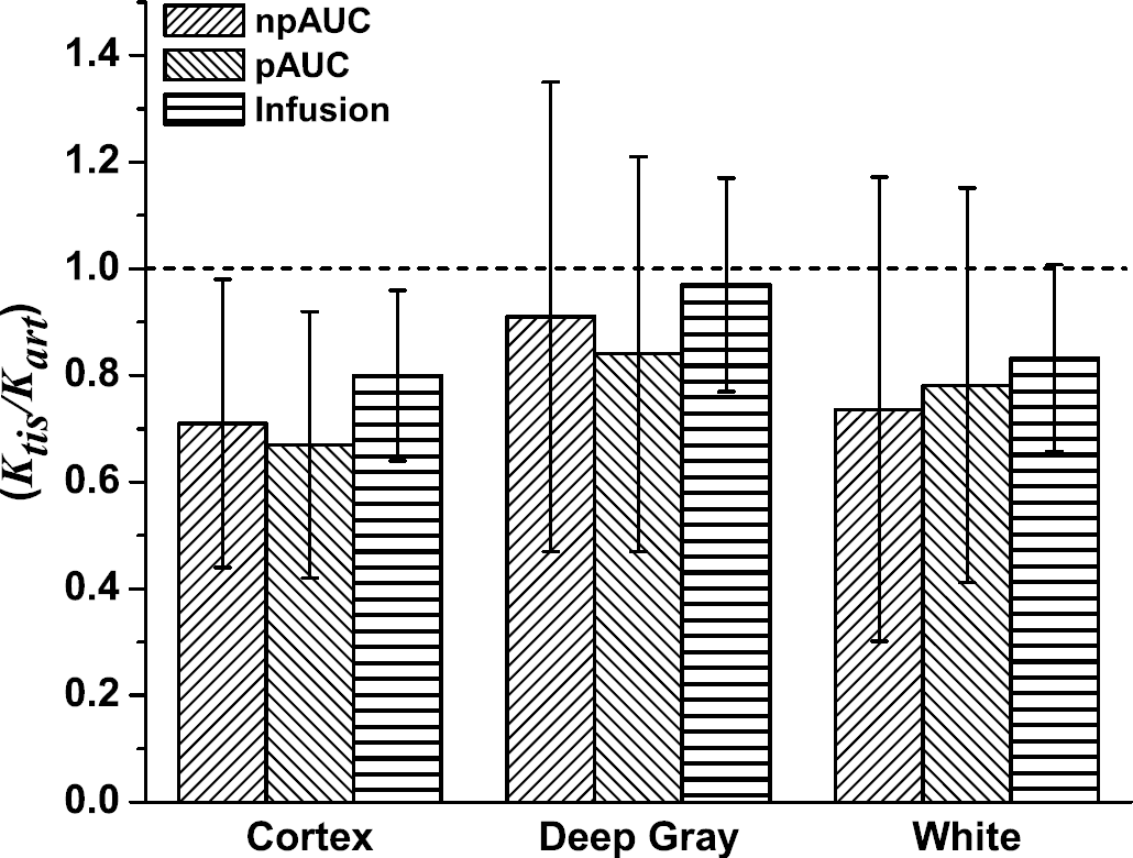
The null hypothesis of this study is that the value of the ratio K_tis/K_art is equal to 1.0 and does not differ among tissue types. The mean ROI values of K_tis/K_art obtained for the nine subjects by all three kinetic methods are given in Table 4 and the mean values for tissue types are shown in Figure 5. It is apparent from this table and figure that deep gray ROIs do not differ from 1.0. However, the ratio is clearly not unity for cortex (P = 0.006 for npAUC; P = 0.003 for pAUC; P = 0.007 for infusion). White matter values of OS K_tis/K_art are similar to those of cortex but, because of the large variance with bolus methods, only the infusion value is significantly different from 1.0 (P = 0.021). The ratios calculated for deep gray differ significantly from both cortex and white matter (Table 5). The values of K_tis/K_art calculated from infusion data are significantly larger than those for either the nonparametric (P = 2.4 × 10⁻⁶) or parametric (P = 2.2 × 10⁻⁷) AUC method. The differences between infusion and nonparametric AUC persist for all three tissue types (cortex, P = 0.008; deep gray, P = 1.4 × 10⁻⁵; white matter, P = 0.017), but only for the gray matter tissue types between infusion and parametric AUC (cortex, P = 0.001; deep gray, P= 0.0002; white matter, P = 0.08). The smaller variance associated with MRI infusion compared with MRI AUC is apparent in the smaller standard deviations of K_tis/K_art tissue means (Figure 5), as well as for the differences between tissue types calculated from Infusion data (Table 5).

Table 4

K_tis/K_art by ROI

ROI	npAUC	ρAUC	Infusion
FC	0.72 ± 0.22	0.68 ± 0.21	0.80 ± 0.20
OC	0.69 ± 0.35	0.64 ± 0.33	0.72 ± 0.19
TC	0.66 ± 0.26	0.64 ± 0.027	0.83 ± 0.28
CD	1.01 ± 0.43	0.96 ± 0.40	0.98 ± 0.21
GP	0.83 ± 0.45	0.80 ± 0.44	0.96 ± 0.19
PUT	0.91 ± 0.40	0.84 ± 0.34	1.04 ± 0.22
TL	0.83 ± 0.51	0.74 ± 0.37	0.89 ± 0.22
AF	0.73 ± 0.38	0.77 ± 0.38	0.80 ± 0.21
OR	0.68 ± 0.40	0.74 ± 0.39	0.85 ± 0.17

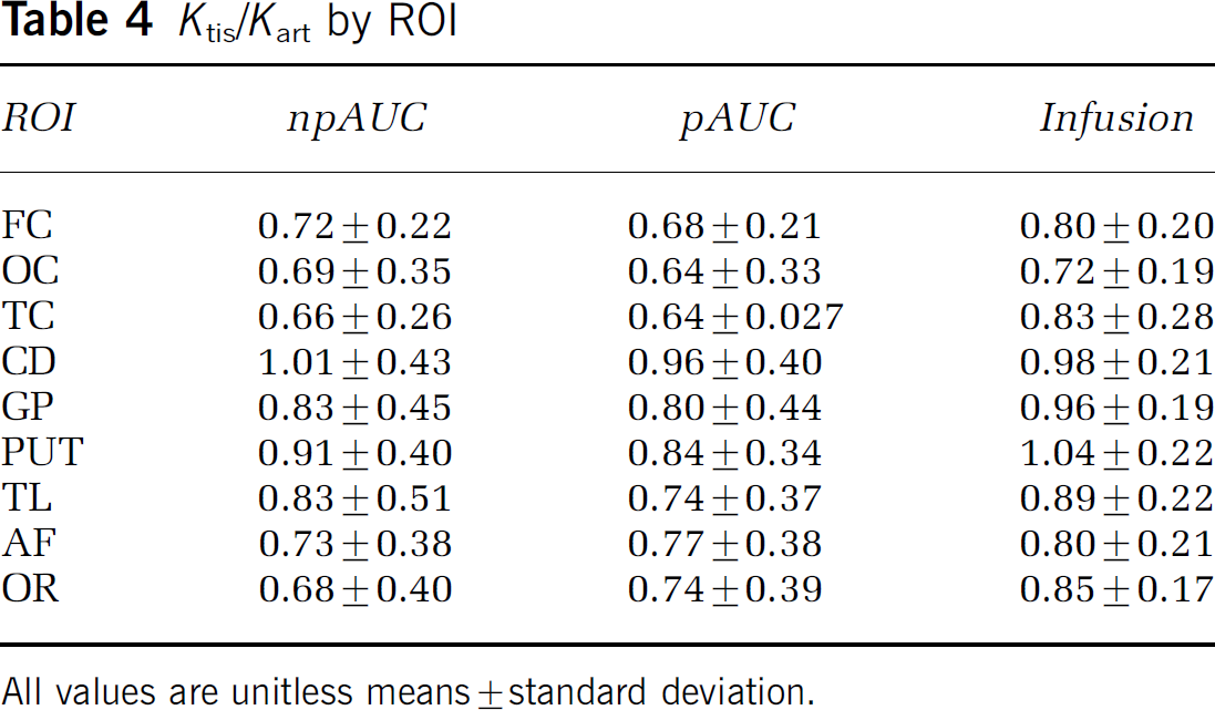
All values are unitless means ± standard deviation.

Figure 5

Ratio of CT/MRI for npAUC and pAUC analyses of bolus data and for infusion by tissue type.

Table 5

Differences for the ratio K_tis/K_art between tissue types by method

Method	Cortex-deep gray		Cortex-white		Deep gray-white

	Mean	P	Mean	P	Mean	P
npAUC	−0.220 ± 0.152	0	−0.024 ± 0.215	0.757	0.178 ± 0.215	0.047
pAUC	−0.215 ± 0.203	0.013	−0.116 ± 0.189	0.311	0.060 ± 0.189	0.245
Infusion	−0.203 ± 0.114	0	−0.036 ± 0.141	0.424	0.142 ± 0.136	0.01

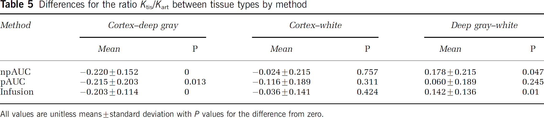
All values are unitless means ± standard deviation with P values for the difference from zero.

The relatively small differences among tissue types for CBV values result in small gray matter/white matter ratios for all methods. The highest ratios occur with infusion kinetics (Table 6).

Table 6

Gray/White ratios by method

npAUC	pAUC	Infusion
CT
1.33 ± 0.14	1.30 ± 0.16	1.35 ± 0.15
MR
1.18 ± 0.27	1.28 ± 0.25	1.29 ± 0.16

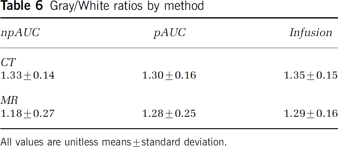
All values are unitless means ± standard deviation.

Contrast to noise ratios of bolus concentration-time curves were approximately 50% larger for MRI than CT in deep gray (34 ± 16 v. 21 ± 7) and white matter (20 ± 7 v. 14 ± 7), although neither difference was significant. In cortex, however, the CNR ratio for MRI was more than twice that for CT (48 ± 24 v. 18 ± 5, P = 0.006). The differences in CNR are illustrated in Figures 6A and 6B, which show the kinetic curves for all pixels in a typical ROI from MRI and CT, along with the curve constructed from the mean value at each time point, analogous to the curves in Figures 1D to 1E and 2D to 2E. The noise envelope of CT data is surprisingly large.

Figure 6

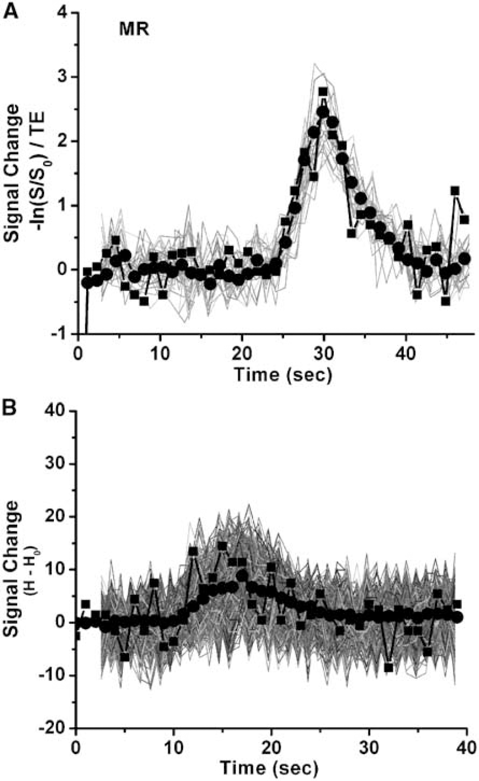
Plots of pixel data for MR (A) and CT (B). Gray lines represent the plot of all pixels in a typical white matter ROI (left optic radiations), squares are the plot of a representative pixel, and circles are the plot of the mean for all pixels. The finer resolution of CT over MR (× 4) results in many more pixels contained in the ROI.

Discussion

These results show that, with dynamic bolus MRI sequences and Gd doses typical for most human studies, the ratio of K_tis/K_art is significantly less than 1 in cerebral cortex and white matter. While also less than 1 in deep gray matter, the difference is not significant. This is consistent with the observed tendency of dynamic contrast T2*-weighted MRI measurements to overestimate CBV (see Table 3 of Newman et al (2003) for summary of the literature). Our estimates of the ratio K_tis/K_art are 0.69 in cortical ROI, 0.87 in deep gray ROI, and 0.76 in white matter ROI, so that the assumption of unity would result in overestimation of CBV by 45%, 15%, and 32% in those regions with the usual AUC integration of T2*-weighted signal change during a Gd bolus. Parametric AUC methods produced larger CBV values in both CT and MRI, slightly greater CBV variance, and slightly smaller values of K_tis/K_art, but the differences from nonparametric results were very small.

Values of K_tis/K_art less than 1 imply that either the tissue integral of contrast over time estimated by MRI is too large relative to CT or the concentration integral of the AIF is too small or both. This is apparent from the expansion and algebraic manipulation of equation (10a):

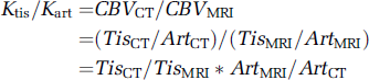
\begin{aligned} K_{t i s} / K_{a r t} & = C B V_{C T} / C B V_{M R I} \\ = (T i s_{C T} / A r t_{C T}) / (T i s_{M R I} / A r t_{M R I}) \\ = T i s_{C T} / T i s_{M R I} * A r t_{M R I} / A r t_{C T} \end{aligned}

(11)

where Tis and Art represent the integral of the contrast agent concentration over time in tissue and artery estimated by CT or MRI for dynamic bolus experiments. Both factors may play a role in the present studies since global differences between bolus and infusion methods across all ROI imply an effect of the AIF, but variation among tissue types suggests a possible influence from the tissue ROI.

A physiologic model of MR contrast due to intravascular magnetic susceptibility perturbations for capillaries and venules in brain parenchyma has been developed by Rosen and co-workers based on randomly distributed, magnetized cylinders with intravascular spins (Boxerman et al, 1995). This Monte Carlo model predicts that T2*-weighted signal change will be linearly dependent on volume fraction, but has nonlinear dependence on contrast concentration. For gradient echo scans with TE of 60 ms, relaxation rate change is predicted to increase quadratically with Gd concentration at low concentrations and then have linear dependence on Gd concentration above 2 mmol/L regardless of the relative weighting of capillaries and venules. Since CT signal change is linear with contrast concentration, it is possible that this quadratic dependence may increase the tissue integral of MRI signal change relative to that of CT and thus contribute to smaller values of K_tis/K_art, Complex MRI phenomenon such as the spread of contrast-induced change in relaxation rate from intravascular spaces to surrounding tissue (‘blooming‘) may contribute to observed regional differences, especially in cortical ROI where leptomeningeal vessels may increase the apparent Gd concentration despite our efforts to avoid this by eliminating the most superficial pixels.

Relating T2* signal change to Gd concentration in an arterial voxel has proven far more difficult, although there has been recent progress (van Osch et al, 2003). As arterial flow within a voxel is neither isotropic nor uniformly distributed, both direction of flow and partial volume averaging influence the signal. The decrease in the blood signal amplitude of a T2*-weighted sequence due to local field inhomogeneities introduced by Gd is described by

| {\vec{S}}_{b} (C_{G d}) | \propto e^{- T E [(1 / T 2 *) + f (C_{G d})]}

(12)

where $\vec{S}$ is the complex MR signal, the value of T2* is for whole blood, TE is echo time, and f is a monotonically increasing function with f(0) = 0 (van Osch et al, 2003). The function f increases linearly with Gd concentration in water, but is expected to increase as a quadratic function in blood (Jensen and Chandra, 2000). The higher magnetic susceptibility due to the presence of contrast inside the artery also will cause a phase shift of the blood signal, which, in theory, varies linearly with concentration. However, if the artery does not fill the voxel, then the total signal change depends on signal from the tissue surrounding the artery, as well as signal from within the artery. If the artery is oriented parallel to the main magnetic field, B_O, then the complex signal arising from the surrounding tissue is independent of the Gd concentration inside the vessel. In this case, the complex signal from the arterial ROI will describe a spiral-like projectory in the complex plane around the static component of the surrounding tissue and it will be possible, at least in principle, to determine f(C_Gd) and calculate the Gd concentration from the amplitude of the signal change. Failure to correct the AIF for these partial volume effects were found to lead to an underestimation of CBV and overestimation of K_tis/K_art, however, so that this would not explain the present findings. If the artery is not parallel to B_O, then it is not possible at present to predict partial volume effects of the surrounding tissue on the arterial signal. Our study used the MCA, which is nearly perpendicular to B_O, so that it is not possible to exclude underestimation of the AIF concentration–time integral due to partial volume averaging. In addition, because van Osch et al (2003) employed comparatively short TE of 9 and 12 ms to avoid approaching signal saturation, it is possible that values of TE between 35 and 60 ms commonly used in the present study and most clinical applications can introduce nonlinear effects, leading to underestimation of the AIF as the arterial signal approached saturation. This is consistent with our own unpublished data, which show reduced sensitivity to Gd at doses above 70 μmol/kg. Finally, there might be unrecognized effects of the vascular ROI pixel selection criteria used.

Values of K_tis/K_art obtained from infusion data were substantially closer to unity, especially for deep gray matter (0.97), but also for cortex (0.80) and white matter (0.83). In addition, the standard deviations of the ratios are much lower with infusions than bolus injections. These findings, together with the observed increase in variability of CBV with bolus MRI (Figure 4, Tables 1 and 2), but a similar variability among tissue types for bolus MRI, are consistent with problems related to the AIF of bolus MRI. Since the MRI infusion technique is actually more sensitive than dynamic bolus to pharmacologically and pathophysiologically induced changes in CBV (Tudorica et al, 2002; Newman et al, 2003), reduced sensitivity to physiological changes cannot explain the higher and more stable K_tis/K_art ratios observed with infusion MRI.

Contrast infusion is theoretically equivalent to a bolus of contrast, but important practical advantages for measurement of CBV reduce the likelihood of an inaccurate AIF. First, because the tissue to artery signals are averaged repeatedly with an infusion, rather than from only a single bolus integral, lower plasma concentrations of Gd are necessary for reliable measurements. With a dynamic bolus, achieving a higher Gd concentration maximizes signal to noise (SNR) within the tissue, but actually decreases SNR in arterial voxels as signal declines toward the intrinsic noise of the measurement. Secondly, infusions minimize the influence of intersubject variability in cardiac output, vascular volume, and other physiologic parameters, which exist even among normal individuals. This further reduces any inaccuracies that might be introduced as the arterial signal approaches the system noise level. Lastly, although partial volume averaging of arterial signal remains an important issue for MRI infusion measurements, the complicated phase angle-amplitude interactions between artery and surrounding tissue, which affect the trajectory of the AIF in the complex plane (van Osch et al, 2003), might be reduced by the more slowly changing concentrations associated with contrast infusion.

Several technical matters require comment. First, measuring CBV by infusion does not obviate the need for a bolus injection since mean transit time and cerebral blood flow measurements require time course data from the bolus. Using the sequences developed for these studies, the combined bolus and infusion paradigm can be accomplished with 250 μmol/kg or less of contrast, well within the FDA-established guidelines of 300 μmol/kg. Unfortunately, at the present time, the inflexibility of existing MRI infusion pumps makes it impossible to execute a single bolus-infusion sequence so that the two scans must be run sequentially and requires manual dilution of contrast for the infusion scan. Elimination of this barrier requires only the availability of a computer-driven pump capable of simultaneous infusion through both feed lines. Secondly, because these studies involved healthy volunteers, additional studies of K_tis/K_art are necessary under conditions of altered blood brain barrier, such as in stroke, tumors, and multiple sclerosis. As the infusion scan involves a 90-sec infusion and 2-min acquisition, it might be more prone to inaccuracy when the blood brain barrier is disrupted than the bolus which requires a 5-sec bolus and 75-sec acquisition. Preliminary studies in acute stroke patients, however, have not identified any significant deviations from the results of the present study. Finally, this study provides no values of K_tis/K_art for the brainstem or cerebellum, and the applicability of the results from the cerebral hemispheres should be established for the posterior fossa as well.

In summary, the assumption that proportionality constants relating signal change to concentration are equal in tissue and artery may contribute to the overestimation of CBV and CBF observed in T2*-weighted MRI studies. The results of the present study provide an estimate of this effect for dynamic contrast MRI sequences commonly used in humans. Infusion MRI yields results that are closer to CT and other methods. Infusion MRI also reduces measurement variability and, thus, may reduce the likelihood of type II errors. There appears to be little advantage of infusion over bolus CT in terms of improved accuracy or reduced variance for CBV measurements.

References

Akbudak

Hsu

Conturo

(1998) ΔR* or Δ9 contrast agent effects in blood. Proceedings of the sixth Annual Meeting ISMRM, Sydney

Axel

(1980) Cerebral blood flow determination by rapid-sequence computed tomography. Radiology 137:679–86

Boxerman

Hamberg

Rosen

Weisskoff

(1995) MR contrast due tointravascular magnetic susceptibility perturbations. Magn Reson Med 34:555–566

Hammer

Kuhn

Meis

. (1995) Quantitative contrast media doseevaluation for cranial computed tomography. Comput Med Imaging Graphics 19:287–93

Jensen

Chandra

(2000) NMR relaxation in tissues with weak magnetic inhomogeneities. Magn Reson Med 44:144–56

Knudsen

Pettigrew

Patlak

Paulson

(1994) Blood-brain barrier permeability measurements by double-indicator method using intravenous injection. Am J Physiol 266:H987–99

Newman

Delucia-Deranja

Tudorica

Hospod

Patlak

(2003) Cerebral blood volume measurements by T2*-weighted MRI and contrast infusion. Magn Reson Med 50:844–55

Nosil

Pearce

Stein

(1989) Linearity and contrast scale control in computed tomography. Med Phys 16:110–3

Perkio

Aronen

Kangasmaki

Liu

Karonen

Savolainen

Østergaard

(2002) Evaluation of four postprocessing methods for determination of cerebral blood volume and mean transit time by dynamic susceptibility contrast imaging. Magn Reson Med 47:973–81

10.

Phelps

Huang

Hoffman

Kuhl

(1979) Validation of tomographic measurement of cerebral blood volume using C-11-labeled carboxyhemoglobin. J Nucl Med 42:1032–9

11.

Smith

Grandin

Duprez

Mataigne

Cosnard

(2000) Whole brain quantitative CBF and CBV measurements using MRI bolus tracking: comparison of methodologies. Magn Reson Med 43:559–64

12.

Tudorica

Hospod

DeLucia-Deranja

Huang

Patlak

Newman

(2002) Cerebral blood volume measurements by rapid contrast infusion and T₂* weighted echo planar MRI. Magn Reson Med 47:1145–57

13.

van Osch

Vonken

Viergever

van der Grond

Bakker

(2003) Measuring the arterial input function with gradient echo sequences. Magn Reson Med 49:1067–76

14.

Weisskoff

Zuo

Boxerman

Rosen

(1994) Microscopic susceptibility variation and transverse relaxation: theory and experiment. Magn Reson Med 31:601

Experimental Estimates of the Constants Relating Signal Change to Contrast Concentration for Cerebral Blood Volume by T2* MRI

Abstract

Keywords

Introduction

Theory

Materials and methods

Subjects and Acquisitions

Image Analysis

Statistics

Results

Discussion

References