Sage Journals: Discover world-class research

Abstract

Voxelwise statistical analysis has become popular in explorative functional brain mapping with fMRI or PET. Usually, results are presented as voxelwise levels of significance (t-maps), and for clusters that survive correction for multiple testing the coordinates of the maximum t-value are reported. Before calculating a voxelwise statistical test, spatial smoothing is required to achieve a reasonable statistical power. Little attention is being given to the fact that smoothing has a nonlinear effect on the voxel variances and thus the local characteristics of a t-map, which becomes most evident after smoothing over different types of tissue. We investigated the related artifacts, for example, white matter peaks whose position depend on the relative variance (variance over contrast) of the surrounding regions, and suggest improving spatial precision with ‘masked contrast images’: color-codes are attributed to the voxelwise contrast, and significant clusters (e.g., detected with statistical parametric mapping, SPM) are enlarged by including contiguous pixels with a contrast above the mean contrast in the original cluster, provided they satisfy P < 0.05. The potential benefit is demonstrated with simulations and data from a [¹¹C]Carfentanil PET study. We conclude that spatial smoothing may lead to critical, sometimes-counterintuitive artifacts in t-maps, especially in subcortical brain regions. If significant clusters are detected, for example, with SPM, the suggested method is one way to improve spatial precision and may give the investigator a more direct sense of the underlying data. Its simplicity and the fact that no further assumptions are needed make it a useful complement for standard methods of statistical mapping.

Keywords

fMRI PET smoothing artifacts statistical parametric mapping

Introduction

Voxelwise statistical analysis has become popular in explorative functional brain mapping (Ashburner et al, 2003) and powerful tools for spatial normalization (Ashburner and Friston, 1999) and statistical analysis (Friston et al, 1995), including correction for multiple testing (Worsley et al, 1992; Friston et al, 1994) are publicly available. In the absence of an anatomically defined a priori hypothesis, statistical tests can be calculated for each voxel after spatial normalization and smoothing. Spatial smoothing is required to cope with interindividual functional anatomic variability that is not compensated by spatial normalization, and to improve the signal-to-noise ratio. Following the matched filter theorem (Rosenfeld and Kak, 1982) that states that the optimal smoothing kernel should match the signal to be detected, smoothing kernels of up to a FWHM (full-width at half-maximum) of 20 mm have been used. Smoothing with an FWHM of 10 to 15 mm is common in PET studies; often smaller kernels are applied in fMRI. The resulting t-maps (t = estimated parameter divided by its standard error) are masked at a certain threshold of voxel-level significance (often P < 0.001), and depicted as an overlay on corresponding anatomic sections, as maximum intensity projections or as surface projections. Those clusters that survive correction for multiple testing are frequently characterized by the coordinates of the maximum t-value and the associated ‘nearest gray matter’. Many of these techniques have originally been developed to detect cortical patterns of neural activation (e.g., with [¹⁵O]H₂O PET or fMRI BOLD signal) and are now increasingly applied also in neuroreceptor/-transporter studies.

It is widely accepted that smoothing limits spatial selectivity and significant clusters are to be interpreted as regional results rather than anatomically precise information. However, little attention is being given to the fact that smoothing affects t-maps differently from ‘contrast images’ (contrast = linear combination of parameter estimates in the general linear model that is supposed to reflect the interesting physiologic parameter). While the latter change with FWHM in a way one might guess intuitively, t-statistics formed from the smoothed data are also affected by the nonlinear interaction of the filter kernel with the voxel variances, which becomes most evident after smoothing over different types of tissue (e.g., gray matter, white matter) with a different variability. Voxelwise maps of parameters such as binding potential have two main sources of variance–-measurement error (all sources of error associated with instrumentation, operator imprecision and the stochastic nature of isotope decay) and authentic between-subject physiologic variance. The physiologic variance can also be decomposed into two main sources–-variance from nuisance variables such as intersubject differences in nonspecific binding, and differences in receptor availability, the variable of interest. The variance attributable to between-subject differences in receptor availability can be considerable, leading to larger variance in gray matter tissues with high receptor density compared with other tissues, especially white matter. If, following smoothing, voxel by voxel statistical tests are performed, spatially inaccurate results may occur because the linear weighting scheme will redistribute voxel variances differently than it redistributes voxel intensities.

The aim of this paper was to demonstrate this effect and to suggest a way of combining t-maps, t-thresholds of significance and contrast images to ‘masked contrast images’ that can be used for presentation and that may allow for a more precise localization of significant effects than t-maps alone. The suggested algorithm was applied to data from a previously published PET study with [¹¹C]Carfentanil that showed subcortical brain regions with increased μ-opiate receptor availability in abstinent alcoholics.

Materials and methods

Theory

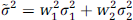
Smoothing is an averaging process in which the intensity at a given voxel is replaced by a weighted average (i.e., a linear combination) of the values of voxels in some spatial neighborhood of that voxel. Common smoothing methods such as Gaussian filtering attribute the most weight to the (pretransformation value of) transformed voxel itself and are symmetric in the sense that the weights then decrease as a continuous function of spatial distance from the transformed voxel location, without any preferred direction (isotropic). A very simple example of such a scheme would consist of a bivariate statistic sampled from two subject groups (i.e., two variables per subject), but analyzed following a transformation such that for each subject, the transformed data associated with each variable is a linear combination of the original two variables. The weighted sum associated with one of the samples, say ỹ would be ỹ = w₁y₁ + w₂y₂ where y_i and w_i are the original samples and weights (i = 1, 2) with standard deviations σ₁and σ₂. If y₁ and y₂ are uncorrelated, the variance of ỹ is given by

{\tilde{σ}}^{2} = w_{1}^{2} σ_{1}^{2} + w_{2}^{2} σ_{2}^{2}

A contrast, for example, a between-group difference Δμ can be tested by a t-statistic; the t-statistics on the transformed variable ỹ, can be expressed in terms of contrasts Δμ₁ and Δμ₂ on each of the original variables y₁ and y₂:

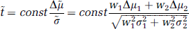
\tilde{t} = c o n s t \frac{Δ \tilde{u}}{\tilde{σ}} = c o n s t \frac{w_{1} Δ μ_{1} + w_{2} Δ μ_{2}}{\sqrt{w_{1}^{2} σ_{1}^{2} + w_{2}^{2} σ_{2}^{2}}}

where const depends only on sample size. On replacing Δμ_i with t_iσ_i/const, one obtains

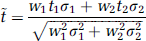
\tilde{t} = \frac{w_{1} t_{1} σ_{1} + w_{2} t_{2} σ_{2}}{\sqrt{w_{1}^{2} σ_{1}^{2} + w_{2}^{2} σ_{2}^{2}}}

(1)

Assuming t₁, t₂ > 0, there is a ratio of weights w₁ and w₂ for which $\tilde{t}$ is maximal. As one can see directly from the vector notation below (equation (9)), this is when w₁ and w₂ correspond to 1/(relative variance) with relative variance being $σ_{i}^{2} / Δ μ_{i}$ :

\frac{w_{1}}{w_{2}} = \frac{t_{1} / σ_{1}}{t_{2} / σ_{2}}

(2)

When the applied weights are proportional to 1/(relative variance), the maximal t-value will be associated with the variable having the smaller relative variance, and thus the ordering of the t-values may be reversed compared with their presmoothed values if the sample with the higher t-value is also the sample with the higher relative variance. The contrast itself is not similarly affected–-if Δμ₁ > Δμ₂ and w₁ > w₂ then the same ordering is preserved in the transformed contrast.

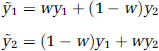
We now seek the range of weights that will lead to a reversal of t-statistic ordering. Given the symmetry of the smoothing kernel and appropriate normalization of the weights (i.e., w₁ + w₂ = 1), ỹ₁ and ỹ₂ can be expressed as

\begin{aligned} {\tilde{y}}_{1} & = w y_{1} + (1 - w) y_{2} \\ {\tilde{y}}_{2} & = (1 - w) y_{1} + w y_{2} \end{aligned}

and, if y₁ and y₂ are uncorrelated, the corresponding t-values ${\tilde{t}}_{1}$ and ${\tilde{t}}_{1}$ are given by equation (1). All weights are positive and as with Gaussian smoothing we assume greater weight in ỹ₁ is given to y₁ than y₂, and vice versa for ỹ₂, thus 0.5 < w < 1. As shown in Appendix A, the ordering of t-values will be reversed if σ₁/t₁ > σ₂/t₂ (thus σ₁ > σ₂) and

0.5 < w < 0.5 + \frac{1}{2} \sqrt{\frac{(σ_{1} / σ_{2} - σ_{2} / σ_{1}) - (t_{1} / t_{2} - t_{2} / t_{1})}{(σ_{1} / σ_{2} - σ_{2} / σ_{1}) + (t_{1} / t_{2} - t_{2} / t_{1})}}

(3)

Next, we extend the discussion to a setting in which the data is defined on a continuous spatial domain and smoothing has been performed. As commonly applied, Gaussian smoothing is linear, isotropic and stationary (independent on position), and so can be represented by convolution ỹ(x) = f(x) ⊗ w(x) with w(x) being the kernel function in the shape of a normal probability density function:

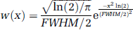
w (x) = \frac{\sqrt{\ln (2) / π}}{F W H M / 2} e^{\frac{- x^{2} \ln (2)}{(F W H M / 2)^{2}}}

(4)

where FWHM denotes the ‘full-width at half-maximum’ of the smoothing kernel.

As a very idealized model for Gaussian smoothed data with two gray matter regions that are small compared with the FWHM of the smoothing kernel and surrounded by white matter with negligible absolute variability, let y₁ and y₂ be two point sources, separated by a distance d. With d₁ being the distance from source one to a given voxel on the line segment between source one and source two, the distance of this voxel to source two is d₂ = d–d₁ and the weights w₁, w₂ attributed to source one and source two are given by equation (4). Together with equation (2), one obtains the position of the maximum t-value:

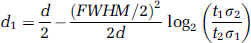
d_{1} = \frac{d}{2} - \frac{(F W H M / 2)^{2}}{2 d} \log_{2} (\frac{t_{1} σ_{2}}{t_{2} σ_{1}})

(5)

For a small FWHM, this is the middle of both point sources. With increasing FWHM, the maximum shifts towards the point source with the lower relative variance.

For imaging data, which can be thought of as a discrete lattice representation of a variable defined on an underlying spatially continuous domain, we expand equation (1) to account for n samples y₁, y₂ … y_n that contribute to a smoothed voxel ỹ(x) (x = three-dimensional voxel coordinate) with the weights w₁(x), w₂(x), …, w_n(x):

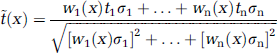
\tilde{t} (x) = \frac{w_{1} (x) t_{1} σ_{1} + \dots + w_{n} (x) t_{n} σ_{n}}{\sqrt{[w_{1} (x) σ_{1}]^{2} + \dots + [w_{n} (x) σ_{n}]^{2}}}

(6)

The assumption for this equation is that all original samples y_i are uncorrelated, which, of course, is not the case for measured voxels. We therefore use y_i to represent independent components of an image rather than voxels. For example, a homogeneous region i with the spatial extent being represented as a voxel mask m_i(x) enters equation (6) as one single sample y_i, and the weight w_i (x) with which it contributes to a smoothed voxel ỹ(x) can be obtained from a convolution of the voxel mask with the smoothing kernel w_s(x):

w_{i} (x) = m_{i} (x) \otimes w_{s} (x)

(7)

Note that the m_i may overlap, corresponding to different regions sharing some component of signal; that is, a voxel x may be a part of one homogenous set of voxels with respect to some component of the signal, and a different set with respect to another component.

The t-value of a smoothed voxel can also be expressed by using the vector notation for equation (6):

\tilde{t} (x) = \vec{t} \cdot \frac{\vec{S} (x)}{∥ \vec{S} (x) ∥}

(8)

where $\vec{t}$ is the n × 1 vector of the original t-values and $\vec{S} (x)$ the n × 1 vector of the weighted standard deviations $w_{1} (x) σ_{1}, w_{2} (x) σ_{2}, \dots, w_{n} (x) σ_{n}$ . As this is an inner product and the length of $\vec{S} (x) / ∥ \vec{S} (x) ∥$ is one, one obtains:

\tilde{t} (x) = ∥ \vec{t} ∥ \cos (ϕ (x))

(9)

where φ(x) is the angle between $\vec{t}$ and $\vec{S} (x)$ . The maximal possible t-value $∥ \vec{t} ∥ = \sqrt{t_{1}^{2} + t_{2}^{2} + \dots + t_{n}^{2}}$ is obtained when $\vec{t}$ and $\vec{S} (x)$ are parallel, that is, when the original samples are weighted with 1/(relative variance). In three-dimensional space and for more than three point sources, this will not, in general, be an obtainable condition and the observed maximum T_max will be below the theoretical maximum $∥ \vec{t} ∥$ . Still, the local maxima of $\tilde{t} (x)$ correspond to local minima of | φ(x) |.

For reasons of simplicity, we do not distinguish between the point spread function w_PSF(x) of the scanner and an additional smoothing kernel applied during image postprocessing w_SPM(x), since, in a typical voxelwise analysis, the former is much smaller and its contribution is negligible. However, one can easily account for both steps of smoothing by defining w_s(x) as the combined kernel w_s(x) = w_PSF(x)⊗w_SPM(x). Assuming w_PSF(x) to have the shape of a bell-curve (as w_SPM(x)), the full-width half-maximum of w_s(x) is given by

F W H M_{t o t a l} = \sqrt{F W H M_{P S F}^{2} + F W H M_{S P M}^{2}}

One-dimensional Simulations

All simulations in this paper were calculated with matlab (Mathworks, Natick, MA, USA). To allow for Monte Carlo simulations with small sample sizes, we did not use equation (6) in the one-dimensional simulation, since equation (6) refers to the true population contrast and standard deviation Δμ and σ and not their estimates from small samples (here, the latter are denoted $Δ \hat{μ}$ and $\hat{σ}$ ). Instead, we calculated a set of unsmoothed one-dimensional ‘images’ f(x) and obtained the smoothed profiles ỹ(x) (each of which is meant to represent smoothed data from one subject) by convolution. A two sample t-test was then calculated from smoothed pixels.

Assuming uncorrelated Gaussian noise ε_pix(x) in each pixel (measurement error) and interindividual variability ε_{reg_i} in each region, f(x) was calculated for two groups of ‘subjects’ (N = 2*1000) from

f (x) = μ_{i} + ε_{{r e g}_{i}} + ε_{p i x} (x)

The corresponding group difference Δμ(x) and the standard deviation $σ_{t o t a l} (x) = \sqrt{σ_{r e g}^{2} + σ_{p i x}^{2} (x)}$ for the first simulation are shown in Figure 1 (‘simulation parameters’). Width and distance of both gray matter regions was d = 10 pixel. For the gray matter regions (gm₁ and gm₂), we assumed a group difference Δμ_gm1 = 1 and Δμ_gm2 = 1.5. Normally distributed random values for ε_pix(x) and ε_{reg_i} were calculated with matlab's function randn() and a standard deviation σ_reg = 1 and σ_pix= 1 (thus σ_total = 1.41) in both gray matter regions. In white matter, no group difference and a lower interindividual variability σ_reg = 0.2 was assumed. The measurement error in white matter was set to $σ_{p i x} = \sqrt{0.2}$ (thus σ_total = 0.49) in accordance with the fact that a lower count rate in PET leads to a lower absolute, but a higher relative statistical error. After Gaussian smoothing with different full-width half-maximum (FWHM = 1, 2, …, 20 pixel), a t-test was calculated for each pixel, and the local maxima of t(x) and $Δ \hat{μ} (x)$ (T_max and $Δ {\hat{μ}}_{max}$ ) were determined for each FWHM by a search algorithm starting in the middle of each gray matter region. For the same setting but a smaller number of subjects (N = 2*10), mean and standard deviation of the position of T_max and $Δ {\hat{μ}}_{max}$ were assessed by Monte Carlo simulation. We also calculated f(x) with different region diameters (d = 3, 4, 5, …, 14 pixel) and obtained the position of T_max from equation (9). For each d we increased the FWHM by steps of 0.1 until T_max shifted into white matter to obtain the ‘critical FWHM’. It should be mentioned that a different number of pixels per region results in a different relative contribution from ε_reg and ε_pix.

Figure 1

Effect of one-dimensional smoothing on t (x), $Δ \hat{μ} (x)$ and $\hat{σ} (x)$ in a pixelwise two sample t-test. Left column: in most pixels, the t-value was increasing with FWHM. The highest increase was found in the white matter between gm₁ and gm₂. For FWHM ⩾ 13 pixel, the t-value there exceeded the t-value in gray matter (arrow). Middle column: The location of the maximum group difference was less affected by spatial smoothing than that of T_max and no additional maximum between gm₁ and gm₂ occurs. Lower right: ‘critical FWHM’ (the FWHM at which a white matter T_max occurs) as a function of the region diameter d (d = width of gm₁, gm₂ and white matter in between).

To further illustrate the artifacts in Figure 1, we chose some modified profiles, including the (idealized) assumption of σ = 0 in the white matter between gm₁ and gm₂. The corresponding Δμ(x) and σ_total(x) are shown in Figure 2. Unless mentioned explicitly, the parameters σ_reg and σ_pixwere the same as in Figure 1.

Figure 2

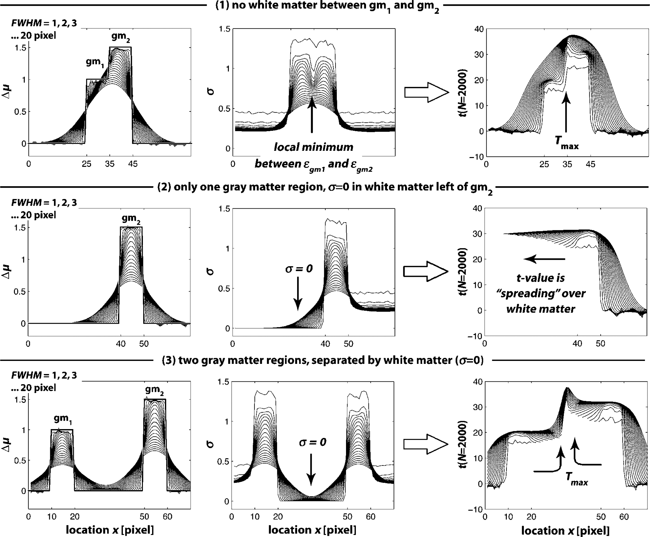
Effects from white matter. The simulation from Figure 1 was modified to illustrate the effects from white matter. Top row: without white matter, smoothing leads to a local minimum of $\hat{σ} (x)$ at the border between gm₁ and gm₂, and to a corresponding peak in t (x) (black arrow). Middle row: Noise and variability in the white matter on the left side from gm₂ was set to zero. After smoothing, the t-value in gm₂ is ‘spreading’ to the left. Bottom row: white matter (σ = 0) allows gm₁ and gm₂ to interfere in spite of a large distance (30 pixel) and create an artificial T_max.

Two-dimensional Simulation

We used a two-dimensional model of three square gray matter regions (5 × 5 pixel each, Figure 3) and surrounding white matter with the same parameters σ_reg (between-subject variability) and σ_pix (measurement error) as in Figure 1. The group difference Δμ was zero in the gray matter region in the middle and was Δμ = 1 in the other two regions. With FWHM = 14 pixel, weights w_i(x) were calculated from equation (7) for all ‘anatomic’ regions (three gray matter regions, one white matter region, standard deviation σ_reg) and additionally for each pixel (standard deviation σ_pix). 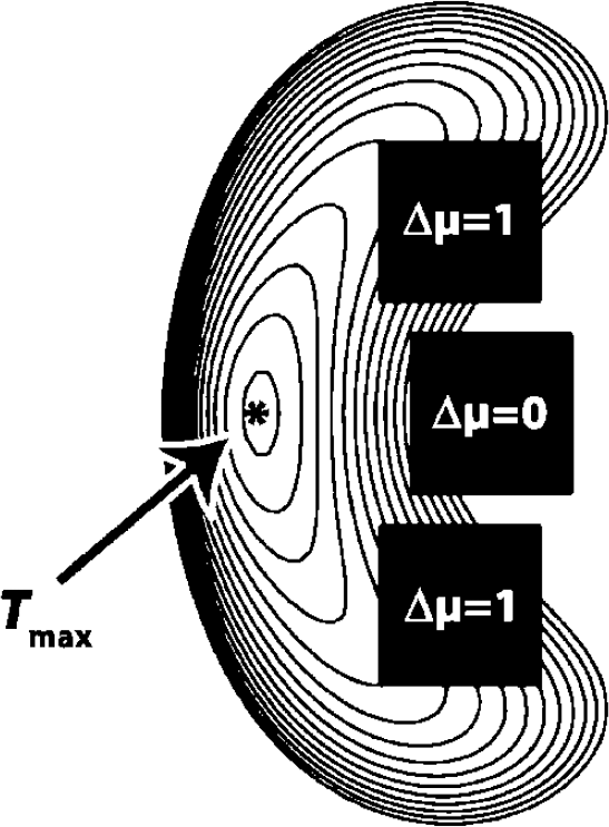The weighted standard deviations $\vec{S} (x)$ were calculated and $\tilde{t} (x)$ was obtained from equation (9). $\tilde{t}$ -isocontours were plotted between 95 and 100% of the observed maximum. For aesthetical reasons, we did not use the same resolution for region mask and smoothed image space, instead, we calculated w_i(x) and $\tilde{t} (x)$ on a much finer grid.

Figure 3

Two-dimensional simulation (worst case): t-isocontours from three gray matter regions (5 × 5 mm = 5 × 5 pixel) and surrounding white matter, smoothed with FWHM = 14 mm. All gray matter regions had the same variance, yet only the upper and the lower region had a positive contrast (Δμ = 1). Note that the nearest gray matter of T_max is the region with Δμ = 0.

[11C]Carfentanil-PET

Measured PET data presented in this paper originate from a previously published PET study in abstinent alcoholics (Heinz et al, 2005). In 20 alcoholics, abstinent for 2 to 3 weeks, and in nine healthy control subjects, radioactivity distribution in the brain was measured with a GE Advance PET-scanner 0 to 66 min after intravenous injection of 700 MBq [¹¹C]Carfentanil, a highly selective μ-opiate receptor ligand. Stereotactically normalized parametric images of receptor availability (Vʺ₃) were calculated with Logan's linearization and the occipital cortex as a reference region with negligible specific binding. For details, see Heinz et al (2005).

SPM Analysis

With SPM2, Vʺ₃ images were smoothed with a 12-mm Gaussian kernel, and a voxelwise two-sample t-test was calculated. Unlike previously published (Heinz et al, 2005), we did not mask out white matter. We applied a voxel-level threshold of P = 0.001 (uncorrected) and confirmed that both striatal suprathreshold clusters survived correction for multiple comparisons with SPM's small volume correction and a mask for the striatal volume of interest (12.1 cm³). The analysis was repeated with a voxel-level threshold of P =0.05 (uncorrected) to obtain the corresponding t-threshold for later use.

Masking Algorithm for Contrast Images

To use contrast images for presentation, just as t-maps with significant clusters being displayed over corresponding anatomic sections, a masking algorithm is needed. Instead of using the original t-isocontours, which are affected by the investigated artifacts, we used a corresponding contrast-threshold that we had calculated separately for each cluster.

The following data were available from the SPM analysis:

t-maps (file: spmT_0002.img).

Contrast images (file: con_0002.img), containing the smoothed ΔVʺ₃.

A list of clusters (coordinates of T_max) that survived SPM's correction for multiple testing.

t-thresholds for P = 0.001 and P = 0.05.

The mask that was applied to SPM's contrast images was calculated as illustrated in Figure 4. For each significant region, we first obtained the original SPM-cluster from t-maps with a region growing algorithm that starts at T_max and includes all voxels with a t-value above the original threshold (here P = 0.001). The mean contrast in this cluster was subsequently used for thresholding and all contiguous voxels that met both the ΔVʺ₃ threshold and satisfied P < 0.05 (to ensure some statistical evidence) were included in the resulting region.

Figure 4

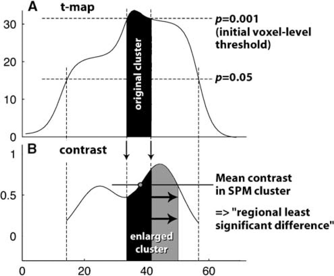
Suggested algorithm to create masked contrast images. (A) For each significant cluster, a mask (black bar) is generated from t-maps and the initial voxel-level t-threshold (P = 0.001) and subsequently applied to contrast images (B). The mean contrast in this cluster is calculated, and the cluster is enlarged by including adjacent voxels (grey area) that exceed this mean contrast. Voxels that do not reach the P = 0.05 level are not included. The depicted profiles were taken from Figure 1 (FWHM =14 pixel).

Results

Simulations

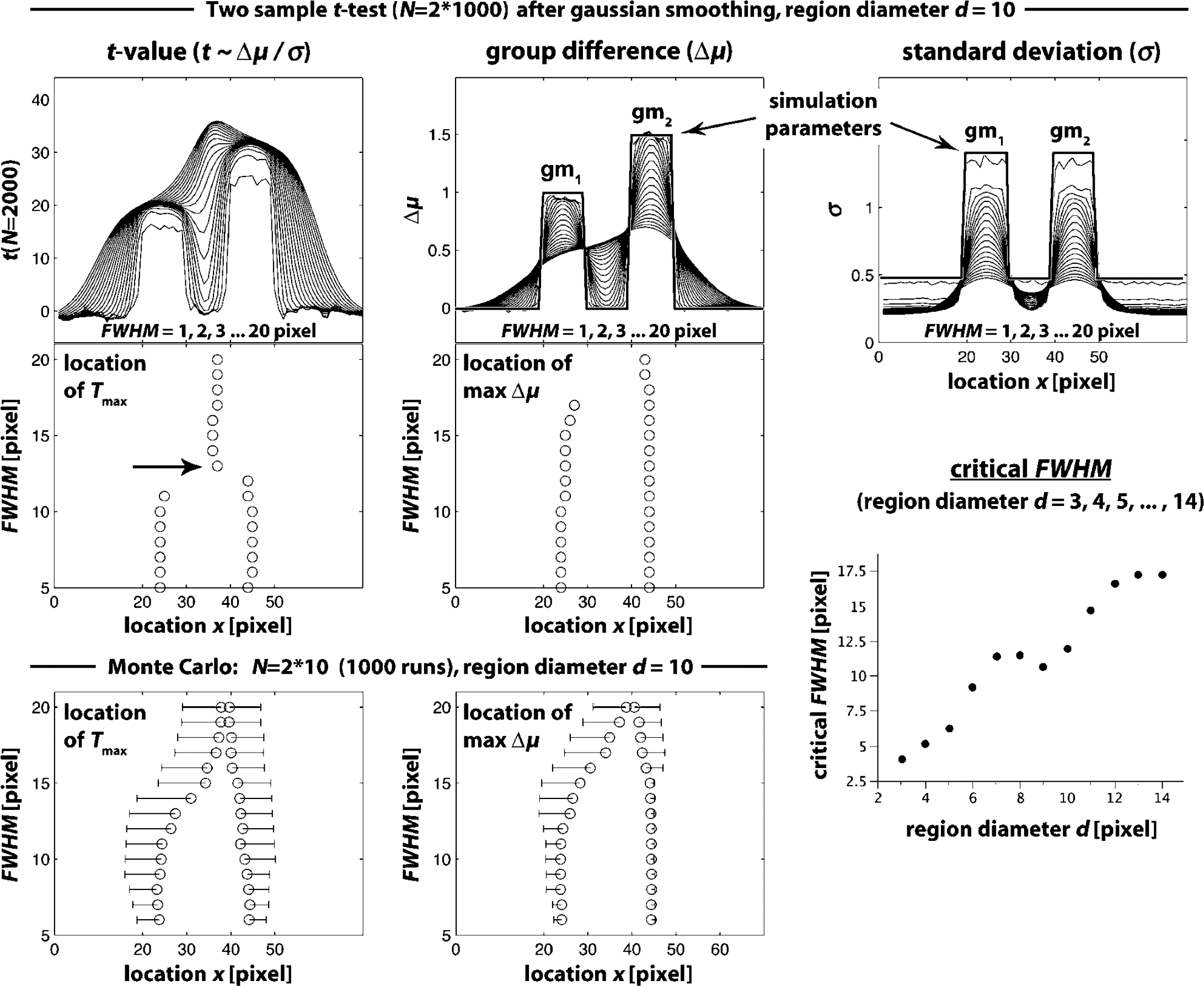
The effect of Gaussian smoothing on t(x), $Δ \hat{μ} (x)$ and $Δ \hat{σ} (x)$ in a pixelwise two sample t-test is shown in Figure 1. In most pixels, the t-value was strictly increasing with FWHM (for FWHM = 3, 4, 5, …, 20). Unlike the shape of $Δ \hat{μ} (x)$ , which changed with FWHM in a way one might guess intuitively, t(x) showed an irregular pattern with the highest increase in the white matter between gm₁ and gm₂ (Figure 1, top left). Slightly decreasing t-values were observed only at higher FWHM (⩾ 10 pixel) at the border between gray and white matter. At FWHM > 12 pixel, there was only one single T_max in the middle of gm₁ and gm₂ (Figure 1, arrow), which slightly shifted back towards gm₂ when FWHM was further increased. The ‘critical FWHM’ at which such a white matter peak occured was lower than 150% of the region diameter d in all simulations (d = 1, 2, 3, …, 14). The position of $Δ {\hat{μ}}_{max}$ was much more stable: the local maximum in gm₁ was preserved until FWHM= 18 pixel, the maximum in gm₂ was located within the gray matter borders until FWHM = 28 pixel (not shown). The higher robustness of $Δ {\hat{μ}}_{max}$ as opposed to T_max was also obvious in the Monte Carlo simulation (Figure 1, bottom): a higher variability of the position of T_max than that of $Δ {\hat{μ}}_{max}$ was observed for all simulated FWHM. At FWHM = 6 pixel, T_max of gm_a was already outside the boundaries of gm₁ in 8% of all realizations.

Results from three modified profiles are depicted in Figure 2:

Without white matter between gm₁ and gm₂ (Figure 2, top row), smoothing resulted in a local minimum in $\hat{σ} (x)$ at the border between gm₁ and gm₂ and a corresponding peak in t(x). When ε_reg was set to zero (but not ε_pix), this peak disappeared (not depicted).

In white matter with a hypothetical variance σ_total = 0 (Figure 2, middle row) and a Δμ = 0, the standard deviation and $Δ \hat{μ}$ after smoothing solely reflect the contribution from the adjacent gm₂. Accordingly, in Figure 2, the t-value left of gm₂ was close to that within gm₂ (theoretically, if gm₂ was only one pixel wide and if the contribution from white matter on the right side of gm₂ was negligible, the t-value would be exactly the same). The horizontal arrow suggests looking at this effect as if the t-value was ‘spreading’ over white matter with increasing FWHM (no t-values were plotted for a denominator $\hat{σ} (x) < 0.001$ ).

When white matter with σ_total = 0 was surrounded by two gray matter regions (Figure 2, bottom row), smoothing resulted in a peak t(x) in the middle of gm₁ and gm₂, which first occurred when both ‘spreading’ t-values met exactly in the middle. For higher FWHM, T_max shifted towards gm₂ (the region with the lower relative variance). Interestingly–-unlike in the simulation without white matter (Figure 2, top row)–-interindividual variability ε_reg (in addition to the measurement error ε_pix) was not needed for this effect.

In the two-dimensional simulation (Figure 3), the maximum t-value was shifted to the left by the gray matter region in the middle (with Δμ = 0). Note that in the chosen setting, T_max was still closer to the gray matter region in the middle than to the regions with a positive contrast.

[11C]Carfentanil PET

SPM analysis of [¹¹C]Carfentanil PET-data confirmed significantly increased μ-opiate receptor availability in the bilateral ventral striatum. Without masking out white matter, the maximum t-value in the left hemisphere was found between ventral striatum and frontal cortex (Figure 5, top left), close to a local minimum of the unsmoothed ΔVʺ₃. Masked contrast images (Figure 5, bottom) were more symmetrical, including more voxels in the middle of the left ventral striatum where the maximum ΔVʺ₃ was found.

Figure 5

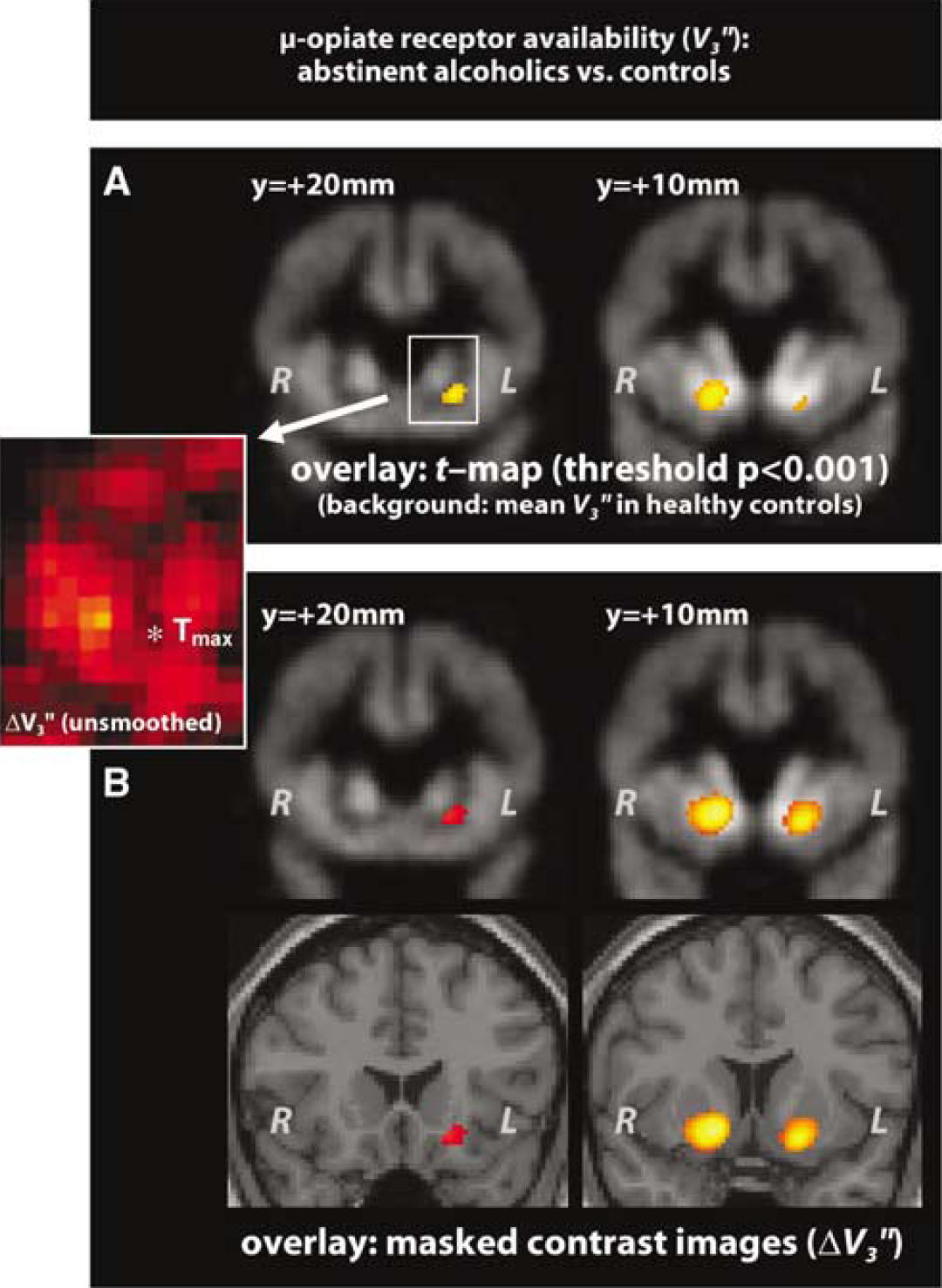
Results from a PET-study with [¹¹C]Carfentanil. μ-opiate-receptor availability Vʺ₃ in abstinent alcoholics was compared with that in healthy controls. (A) Traditionally thresholded t-maps show significantly elevated Vʺ₃ in the bilateral ventral striatum. However, the maximum t-value of the left cluster was found in adjacent white matter (y = +20 mm), near the local minimum of unsmoothed ΔVʺ₃ (see inset, T_max = white star ‘*’). (B) SPM's contrast images (smoothed ΔVʺ₃), masked as described, show a more symmetrical pattern with a T_max within the borders of the bilateral ventral striatum (y = + 10 mm).

In the right striatum, group differences were stronger and the standard deviation showed less local variation. Accordingly, masked contrast images were very similar to the original t-map.

Discussion

In addition to the loss of resolution that is inherent in spatial smoothing, the nonlinear interactions with the voxel variances (which affect t-maps, but not contrast images) can result in sometimes-counterintuitive artifacts, as demonstrated in this paper. These effects include a displacement of T_max away from a region with a higher relative variance, and a displacement of T_max towards the middle of two or more regions with a positive contrast and independent error terms. In the latter case, a displaced peak differs from a smooth, combined peak in contrast images in that it manifests at much lower levels of smoothing, and is spatially narrowed in a manner such that it may be mistakenly identified as an additional finding. The position of this peak depends on the relative variances of the surrounding regions so that the ‘nearest gray matter’ algorithm may not always determine the correct anatomic region.

This can be understood by looking at two effects:

smoothing causes the independent error terms of two or more neighboring gray matter regions to be averaged, resulting in a minimum variance between these regions

white matter with little statistical noise and low absolute interindividual variability ‘inherits’ the t-value of adjacent gray matter, and peaks in t-maps may become broader than the corresponding peaks in contrast images. This not only leads to a higher uncertainty of the position of T_max (as demonstrated in the Monte Carlo simulation), white matter also may serve as a ‘bridge’ between two or more interacting gray matter regions.

In our one-dimensional simulation, Gaussian smoothing with an FWHM in the same order of magnitude as the distance of the involved regions was already critical. Depending on the actual structure, this effect may even be stronger after three-dimensional smoothing. While such a t-shift is less likely to affect functional mapping of the cortex, it may seriously impair localization of subcortical findings, as for example, in the presented PET study with [¹¹C]Carfentanil, where a maximum t-value was observed in the white matter between ventral striatum (where higher μ-receptor availability was expected) and the frontal cortex (where alcoholics also displayed a higher μ-receptor availability, though not significant). Smaller misplacements may just be an aesthetical concern or may raise the question of how to present the results in a convincing way. Larger misplacements may get masked out (white matter mask) at the expense of sensitivity. Findings may also go undetected when the T_max shifts into a neighboring gray matter region with lower relative variance. Finally, misinterpretations may occur in brain areas with more than two gray matter regions, as in our two-dimensional (worst case) simulation, where the ‘nearest gray matter’ algorithm would not have detected the two regions that contributed to T_max. Likewise, one has to be careful when assigning peaks to functional subunits, for example, of the thalamus or the ventral striatum.

In the literature, different smoothing kernels are usually compared with regard to the sensitivity of detecting significant regions (Hopfinger et al, 2000). Using a spatially stationary noise model, Worsley et al (1996) also describe the effect on the local characteristic of the t-map, notably a broadened peak between the two original maxima. However, the most striking effects, including a narrowly focused but shifted peak as in our simulations, only occur when estimating a local variance (Friston et al, 1991) instead of a pooled variance across voxels (Worsley et al, 1992), and when smoothing across different types of tissue. To our knowledge, these effects have not yet been investigated in the literature.

Several methods have been suggested to improve spatial precision of statistical maps. Clearly, reanalyzing the data with a smaller smoothing kernel (Worsley et al, 1996) would have reduced the described artifacts, but at the expense of statistical significance. Another approach is to incorporate spatial a priori assumptions. Davatzikos et al (2001) have described an atlas-based adaptive smoothing to avoid smoothing across anatomic boundaries, which theoretically prevents the described artifacts. However, including a priori information either increases the complexity of the analysis or limits the advantages of a voxel-based (no a priori assumptions) over traditional ROI analysis. Accordingly, ‘classical statistical maps’ (Penny and Friston, 2004) are still the most popular approach for explorative imaging.

While all established methods have in common that the reported values are statistical measures related to a level of confidence by which a ‘true effect’ was observed, the method suggested in this paper follows a different rationale. We do rely on established methods of statistical mapping (in particular those implemented in SPM2, however, other methods as a starting point are also possible) to detect significant regions, but once a cluster is considered significant, we suggest attributing voxelwise color-codes to the estimated parameter itself instead of the level of confidence by which it is greater than zero.

The limitations of the presented method are those of any voxel-based analysis. They are powerful tools for explorative imaging, but they are not necessarily a replacement for traditional region-of-interest (ROI) analysis when a regional a priori hypothesis exists and when an ROI definition is anatomically and physiologically justified. Comparing voxel-based with ROI-based analyses is not subject of this paper, but it should be mentioned that the proposed method was primarily developed for assessment of subcortical regions for which an ROI analysis may indeed be a more straightforward approach. In voxel-based analyses, the type I error must be reduced by using a rather conservative voxel-level threshold (e.g., P < 0.001), which may result in a loss of statistical power. Applying such a single t-threshold as a first step has shown to be a simple and powerful method to detect significant clusters (e.g., by considering the cluster size). However, such a t-threshold is not necessarily the best choice to determine the outline of a neurobiologic effect, which leaves room for other methods of masking such as the one presented in this paper. Using the contrast for color-coding, it may seem natural to use it also to define the outline of a displayed region. Indeed, we have shown that this may provide further information about the locus of, for example, a group difference, albeit in an exploratory form outside the framework of hypothesis testing. It should be noted that our masked contrast images differ from the original thresholded t-maps only if there is a local variation in the variance of the smoothed voxels. The suggested method can therefore be understood as an attempt to stick closely with the current standards while removing the described smoothing artifacts.

We believe that adding a further step to the analysis by going from thresholded t-maps to masked contrast images does not substantially increase the overall complexity of the analysis. On the contrary, it may give the investigator a more direct sense of the underlying data and may improve spatial precision when a significant region occurs. The simplicity of the suggested method and the fact that we do not make further assumptions make it a useful complement for established methods for statistical mapping.

Footnotes

Appendix A

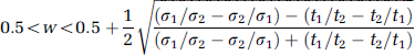
We seek the values of w, 0.5 < w < 1, such that ${\tilde{t}}_{2}$ > ${\tilde{t}}_{1}$ while t₁ > t₂, or DIF(w) = ${\tilde{t}}_{1}$ − ${\tilde{t}}_{2}$ < 0.

Note that DIF(0.5) = 0, and DIF(1) = t₁ – t₂ > 0, and DIF is a differentiable function of w. The derivative, evaluated at w = 0.5 is

and this will be negative (i.e., DIF(w) will be negative immediately to the right of w = 0.5) when σ₁/t₁ > σ₂/t₂.

Therefore, if this condition pertains and DIF(w) has exactly one root in the open interval (0.5, 1), it must be the case that DIF is negative between 0.5 and the root, and positive between the root and 1, and the ordering of the t-map will be reversed compared with the original values on the interval 0.5 < w < root.

We therefore seek to show that DIF(w) has exactly one root between 0.5 and 1. DIF = 0 is equivalent to ${\tilde{t}}_{1}^{2} = {\tilde{t}}_{1}^{2}$ (for $\tilde{t}$ > 0), which can be written as

with

This leads to a cubic equation in w (the 4th power term cancels). Noting that 0.5 is a solution of equation (A1), the remaining two solutions of equation (A1) are the roots of the quadratic

These roots, in terms of the original variables, are

Finally, given the conditions on t₁ t₂, ${\tilde{t}}_{1}$ and ${\tilde{t}}_{2}$ , the expression under the radical sign must be between 0 and 1, and therefore the larger of the 2 roots falls between 0.5 and 1, and is the only solution to equation (A1) in that interval. Values of w falling between 0.5 and the larger root of equation (A1) will lead to a reversal of the ordering of the t-values.

References

Ashburner

Friston

(1999) Nonlinear spatial normalization using basis functions. Hum Brain Mapping 7:254–66

Ashburner

Friston

Penni

(eds) (2003) Human Brain Function, 2nd ed, Chapt. Part II—Imaging Neuroscience—Theory and Analysis. Amsterdam: Elsevier

Davatzikos

Herskovits

Resnick

(2001) Accuracy and sensitivity of detection of activation foci in the brain via statistical parametric mapping: a study using a PET simulator. Neuroimage 13:176–84

Friston

Frith

Liddle

Frackowiak

RSJ

(1991) Comparing functional (PET) images: the assessment of significant change. J Cereb Blood Flow Metab 11:690–9

Friston

Holmes

Worsley

Poline

Frith

Frackowiak

RSJ

(1995) Statistical parametric maps in functional imaging: a general linear approach. Hum Brain Mapping 2:189–210

Friston

Worsley

Frackowiak

RSJ

Mazziotta

Evans

(1994) Assessing the significance of focal activations using their spatial extent. Hum Brain Mapping 1:214–20

Heinz

Reimold

Wrase

Hermann

Croissant

Mundle

Dohmen

Braus

Schumann

Machulla

H-J

Bares

Mann

(2005) Stable elevations in striatal μ-opioid receptor availability in detoxified alcoholics correlate with alcohol craving a [¹¹C]Carfentanil PET study. Arch Gen Psychol 62:57–64

Hopfinger

Büchel

Holmes

Friston

(2000) A study of analysis parameters that influence the sensitivity of event-related fMRI analyses. Neuroimage 11:326–33

Penny

Friston

(2004) Classical and Bayesian inference in fMRI. In: Advanced Image Processing in Magnetic Resonance Imaging ( Landini

, ed) New York: Marcel Dekker

10.

Rosenfeld

Kak

(1982) Digital Picture Processing. New York: Academic Press

11.

Worsley

Evans

Marret

Neelin

(1992) Three-dimensional statistical analysis for CBF activation studies in human brain. J Cereb Blood Flow Metab 12:900–1180

12.

Worsley

Marrett

Neelin

Evans

(1996) Searching scale space for activation in PET images. Hum Brain Mapping 4:74–90

Effect of Spatial Smoothing on t -Maps: Arguments for Going Back from t -Maps to Masked Contrast Images

Abstract

Keywords

Introduction

Materials and methods

Theory

One-dimensional Simulations

Two-dimensional Simulation

[11C]Carfentanil-PET

SPM Analysis

Masking Algorithm for Contrast Images

Results

Simulations

[11C]Carfentanil PET

Discussion

Footnotes

Appendix A

References