Sage Journals: Discover world-class research

Abstract

Objective

Standard-of-practice search management requires that the probability of detection (POD) be determined for each search resource after a task. To calculate the POD, a detection index (W) is obtained by field experiments. Because of the complexities of the land environment, search planners need a way to estimate the value of W without conducting formal experiments. We demonstrate a robust empirical correlation between detection range (Rd) and W, and argue that Rd may reliably be used as a quick field estimate for W.

Methods

We obtained the average maximum detection range (AMDR), Rd, and W values from 10 detection experiments conducted throughout North America. We measured the correlation between Rd and W, and tested whether the apparent relationship between W and Rd was statistically significant.

Results

On average we found W ≈ 1.645 × Rd with a strong correlation (R² = .827). The high-visibility class had W ≈ 1.773 × Rd (also R² = .867), the medium-visibility class had W ≈ 1.556 × Rd (R² = .560), and the low-visibility had a correction factor of 1.135 (R² = .319) for Rd to W. Using analysis of variance and post hoc testing, only the high- and low-visibility classes were significantly different from each other (P < .01). We also found a high correlation between the AMDR and Rd (R² = .9974).

Conclusions

Although additional experiments are required for the medium- and low-visibility search objects and in the dry-domain ecoregion, we suggest search planners use the following correction factors to convert field-measured Rd to an estimate of the effective sweep width (W): high-visibility W = 1.8 × Rd; medium-visibility W = 1.6 × Rd; and low-visibility W = 1.1 × Rd.

Keywords

search and rescue SAR range of detection effective sweep width probability of detection search theory missing persons

Introduction

The Introduction briefly reviews the difficulty applying formal search theory to wilderness search, and the progress since the late 1990s. The Methods section presents the experiments and statistical analyses in detail, as appropriate for an archival scientific paper. The wilderness practitioner willing to forego statistical rigor or theoretical background could begin with the Conclusions or Discussion and work backward to check details.

Search theory as a formal scientific discipline was established during the Second World War by Koopman.^1,2 A searcher must both look in the correct location and be able to detect the search object. However, the location of the subject is unknown, and even looking in the correct location does not guarantee a detection. Search theory contends with this uncertainty by deploying available resources to achieve the maximum probability of success (POS) in the minimum time. The formula that expresses this relationship is OPOS = ∑ POS = ∑ (POD × POA).³ That is, the overall probability of success (OPOS) is the sum over tasks of the probability of detection (POD) times the probability of area (POA). The ultimate goal of search theory is the optimal allocation of search resources. This requires determining the POD, probability of containment (POC) or POA, search area, and searcher speed. The development of search theory has been described in detail by Frost.⁴ ^–7 The POA in the land environment can be determined through the use of statistical models based on previous incidents,⁸^–10 models that use Monte Carlo simulation of search object movement through the environment,¹¹ subject matter expert input from a consensus method,⁶ or by combining all of the above.¹² In the land environment another challenge is quantifying the POD.

No matter what environment, the POD depends on coverage. Coverage depends on 3 factors: the amount of effort expended in searching the area, the size of the area where the effort was expended, and the detection index or effective sweep width (ESW). A precise mathematical formula to calculate the POD from these factors is readily available.⁵ ^,13–15 Additional work describing POD can be obtained from Stone.¹⁶ The difficulty in actually implementing the theory in the land environment has always been determining the value of the detection index or W. In the maritime and aeronautical search environments, W tables are readily available¹⁷ thanks to extensive actual detection experiments done by the US Navy and US Coast Guard to determine key factors.¹⁸ These tables take into consideration the 3 factors that determine W: the nature of the searcher (or sensor), the nature of the search object, and the environment between the 2. Actual field experiments are the only method to determine the lateral range curve, which shows the cumulative probability of a detection for all the search objects at various distances. The distance used is the closest point of approach along the track to the search object.⁴ Once the lateral range curve is experimentally derived, it can be reduced to a single number (W) by either determining the area under the curve or using the crossover technique.¹⁹ The crossover technique has been shown to be highly reliable and has been used to determine W on all 10 of the land visual experiments.¹³^,14,19

Unfortunately, the land environment is far more complex and variable than the maritime environment. Bailey²⁰ and McNab et al²¹ have identified 52 distinct ecoregions at the province level in North America and 190 sections in the contiguous United States. Mountainous regions are subject to altitudinal zonation and introduce additional complexity. Within each section can be 16 classes based on the National Land Cover Database 2006 (NLCD2006).²² Although only 7 of the 16 classes would be expected to vary for each ecoregion section, this still leaves 1330 possibilities without considering seasonal differences. Even within each ecoregion section, the density of vegetation can change, which will affect detectability.²⁰ Therefore, a simple set of tables to provide W values in the land environment for visual search is not likely.

Because of the lag in adaptation of any new method and the lack of W data for local environments, most search efforts continue to use POD figures estimated by field searchers. Previous research has demonstrated that trained searchers are unable to estimate their POD values.^13,14 Early landmark experiments by Wartes in detection provided a POD value based on between-searcher spacing.²³ A decade later Perkins and Roberts developed a concept called critical separation (CS) that accounted for the search object, environment, and searcher. It also predicted POD based on between-searcher spacing.²⁴ However, as pointed out in a review of land search literature, these early papers did not account for search effort (formally defined as the sum of the distance traveled by each search resource within a search segment).¹⁵ Wartes later reconsidered his position (POD based on between-searcher spacing) and recanted the POD as a function of spacing approach.²⁵ Importantly, the gold-standard method of calculating a retrospective POD—multiplying total track line length (effort) by local effective sweep width (W) values to obtain the area effectively swept, then dividing the result by the area of the searched segment to calculate coverage⁵—depends on determining W, currently through a time-consuming, labor-intensive setup of a local ESW experiment. In the absence of a previous W experiment, this effort is simply not possible when a lost-person incident has begun. The land search-and-rescue (SAR) community, therefore, could benefit greatly from a simple, objective procedure that obtains W values without conducting full-blown detection experiments.

Methods

Definitions

Area Effectively Swept (Z/AES)—Previously defined as the product of the total track length (TTL) of all searcher paths in the area searched and the sweep width (W): AES = TTL × W.¹⁴

Average Maximum Detection Range (AMDR)—An experimental process that involves obtaining both the average range of detection (Rd) and the average range of extinction (Re) from 8 legs (angles).¹⁴

Coverage (C)—Previously defined as the ratio of the area effectively swept (AES) to the area searched (A): C = AES/A.¹⁴

Effective Sweep Width (ESW)—Previously defined as either the area under the lateral range curve or the distance in which the number of detections equals the number of missed detections. In this paper ESW denotes the experimental process for measuring, and W denotes the value measured (see W).¹⁴

Probability of Area/Containment (POA/POC)—Previously defined with both terms being identical. The terms refer to the probability of the search object being in a given defined geographic space. The term POA is typically used by the wilderness community and the term POC is used by the aeronautical and maritime community.²⁶

Range of Detection (Rd)—The average of linear distances at which a search object is first detected when moving toward it from multiple angles.

Range of Extinction (Re)—The average of linear distances at which a search object is no longer seen after it has been detected while moving away from it from multiple angles.

Search Visibility Class—A broad description of the amount of contrast between the search object and the environment. Search objects were placed into 1 of 3 classes; high visibility, medium visibility, or low visibility.

Sweep Width (W)—The numerical value in units of linear distance that represents a given object’s detectability with a given sensor operating in a given set of environmental conditions; determined from an ESW experiment (see ESW). Also called effective sweep width.¹⁴ The word sweep in this context is not to be confused with its common use in expressions like sweep [search] an area, perform n sweeps of an area, sweep searching (as a tactic), and so on.

ESW Experiments

A total of 10 ESW experiments have been conducted by 3 separate research teams. Each experiment is shown in Table 1. The data derived for this paper’s analysis come from these experiments conducted around North America. The methodology for the first 5 experiments is described by Koester et al.¹⁴ In all of these experiments the AMDR distance was determined by collecting 16 measurements (Figure 1). The measurements consisted of an Rd, when the search object was first detected, and the Re, when the object once located could no longer be detected. The AMDR value is not the maximum distance at which the search object can be detected from any angle but instead an average of both Re and Rd. The Rd value will almost always be less than the AMDR value except in the rare case when Rd equals Re from every angle. AMDR measurements used either a tape measure or an electronic rangefinder with precision ± 0.5 m (different models of the Nikon rangefinder were used). All AMDR distance measurements were taken on the experimental courses by the research team. The AMDR distance measurement was always taken before the experiment, which ranged from a week to a day before the experiment, and was entered into the Integrated Detection Experiment Assistant (IDEA) worksheet.²⁸

Table 1

Location and characteristics of effective sweep width experiments

Source	Location	State	EcoRegion	Province	Terrain	Season
Koester et al.¹⁴	Shenandoah National Park	VA	M221	Central Appalachian Broadleaf Forest	Mountainous	Winter
Koester et al.	Gifford National Forest	WA	M242	Cascade Mixed Forest	Flat	Summer
Koester et al.	Lansdowne	VA	231	Southeastern Mixed Forest	Flat	Summer
Koester et al.	Lincoln National Forest	NM	M311	Great Plains Steppe and Shrub	Mountainous	Spring
Koester et al.	Mt. Diablo State Park	CA	M261	California Coastal Chaparral Forest and Shrub	Mountainous	Summer
Chiacchia et al. (in preparation)	Manheim	PA	M221	Central Appalachian Broadleaf Forest	Mountainous	Spring
Chiacchia and Houlahan¹³	State Game Land 203	PA	220	Eastern Broadleaf Forest (continental)	Hills	Winter
Twardy²⁷	Mt. Greylock	MA	M210	Adirondack-New England Mixed Forest	Mountainous	Summer
Chiacchia and Houlahan	State Game Land 203	PA	220	Eastern Broadleaf Forest (continental)	Hills	Summer
Chiacchia et al. (in preparation)	State Game Land 203	PA	220	Eastern Broadleaf Forest (continental)	Hills	Summer

Figure 1

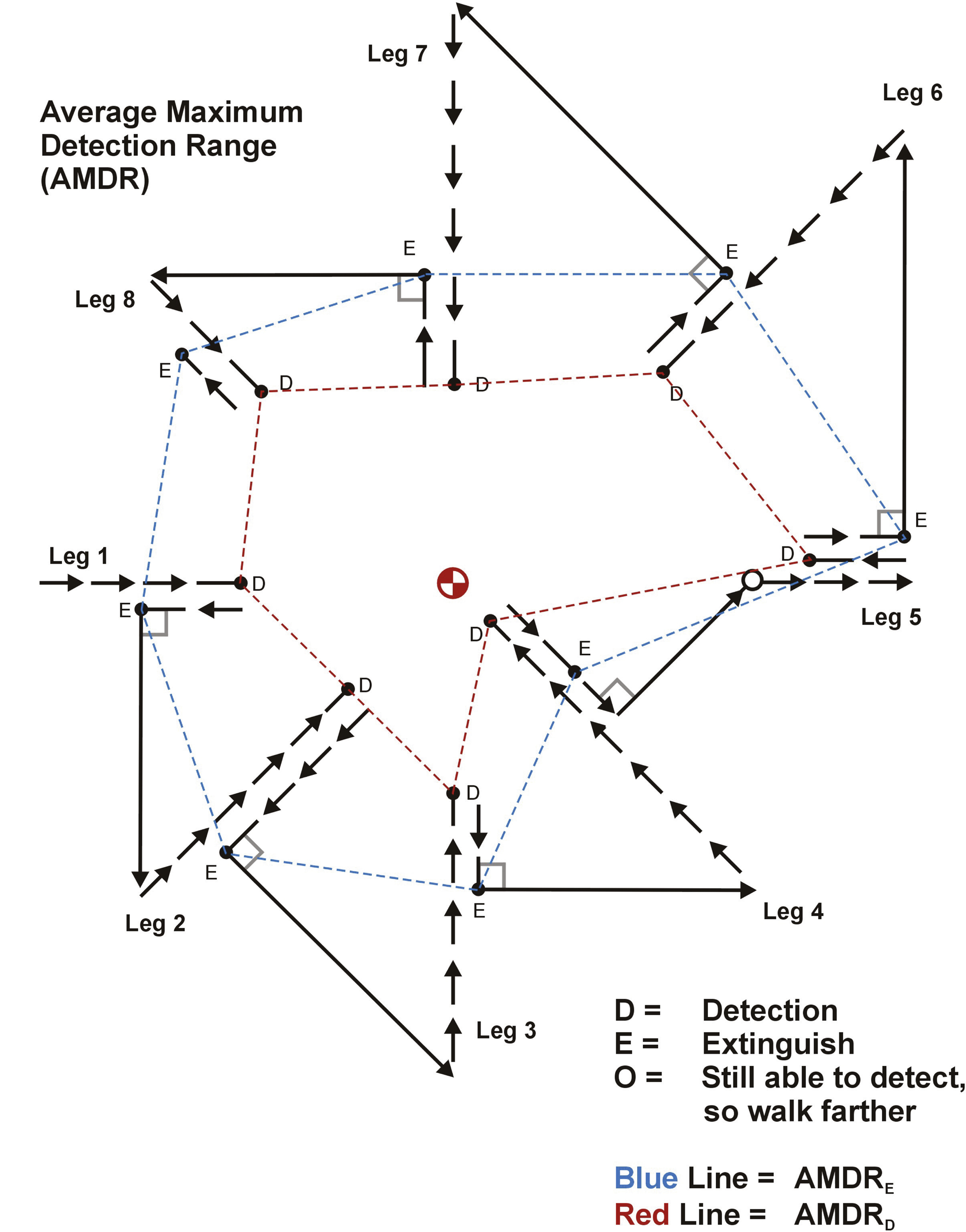
Procedure to determine average maximum detection range (AMDR).

The worksheet then automatically generated a randomized plan for the ESW course. Search objects were high-visibility manikins (stuffed white coveralls with orange safety vests), medium-visibility manikins (stuffed dark blue coveralls), or low-visibility manikins (stuffed olive drab coveralls). In addition, gloves were used for clue-sized objects. Gloves were either high-visibility (Day-Glo orange or royal blue) or low-visibility (dark brown or painted olive). Searchers then walked the track, made detections, and a data collector recorded all detections. All 10 experiments were conducted in the daytime. After the experiment, detections and misses were entered into the IDEA worksheet, and the software provided the W value using the crossover technique.^14,19

The first 5 experiments were conducted by Koester et al¹⁴ and documented in a US Coast Guard report. Subsequent ESW experiments used a refined version of IDEA, and made small changes as required by local conditions.²⁸ Experiment 6 was held at Manheim, Pennsylvania. Half of the experimental team from Koester et al¹⁴ observed and provided assistance to the new team led by Chiacchia et al. (manuscript in preparation). The seventh experiment was conducted at Mt Greylock in the Berkshire Mountains of Massachusetts.²⁷ The course was set up by Twardy and Frost (a member of the experimental team from Koester et al). They deviated from the method in the following ways: they had only 3 targets, the high-visibility adult manikin, assorted white shoes for high-visibility clues, and assorted brown or black shoes for low-visibility clues.

The remaining 3 experiments were all conducted in the northern part of State Game Lands 203 in Marshall Township, Pennsylvania, led by Chiacchia. The results of 3 of those experiments were reported by Chiacchia and Houlahan¹³ along with the slight modification they made to the methodology. The changes to the methodology included one versus two AMDR process estimate, use of manufacturer-dyed brown, royal blue, and orange gloves versus spray-painting white gloves, slight modification of lateral range for search object location, and modification of some of the forms. (Chiacchia’s 2010 course was calibrated using figures from the 2008 experiment, but used manufacturer-dyed gloves of much different hue. Therefore, on August 24, 2011, Chiacchia and Houlahan obtained AMDR and Rd distances for the objects used in the 2010 experiment. We use these data to ensure an apples-to-apples comparison.)

Statistical Analysis

To conduct the analysis for this paper, the raw data and results from IDEA were obtained from each of the 10 experiments. Before analysis, each search object was classified as either high visibility, medium visibility, or low visibility by visual contrast. The high-visibility class included orange gloves, white shoes, and white or orange adult-size manikins, and high-contrast royal blue gloves used in 1 experiment. The AMDR value and W value were recorded from IDEA. All results were entered into a Microsoft Excel spreadsheet. (Note that the W values reported in the current study from Chiacchia and Houlahan are those obtained by pooling data from all their searchers, and so differ slightly from W values reported in that study, which were median or mean values of W calculated for individual searchers.¹³)

We performed statistical analysis 1) to find the 95% CIs for our parameters, and 2) to determine whether relationships were statistically significant. We performed our tests using GraphPad Prism version 5.04 for Windows (GraphPad Software, San Diego, CA, www.graphpad.com). All tests were 2-tailed. Trends were subjected to a least-squares analysis using a linear function with the y-intercept constrained to 0. To compare the slope parameters so derived, the values, standard errors, and degrees of freedom from these analyses were in turn used to perform either analysis of variance (ANOVA—when more than 2 values were being compared) or a parametric t test (when 2 values were compared). Note that to perform this calculation, we added 1 to each degree of freedom value to regenerate the correct n.²⁹ For the ANOVA results, individual differences were subjected to a Tukey’s multiple comparison test, with the minimum significance level set to P ≤ .05 (note, however, that the software identifies higher levels of significance as well). All graphs show uncertainties as standard deviations.

This particular study was conducted using preexisting data taken from IDEA software generated during previous detection experiments. None of the data uniquely identified any individual that participated in the experiments. Instead, the W values are composite values obtained by aggregating all individual results. The AMDR values and hence Rd values were obtained by members of the research team, all of whom are also members of SAR teams and well-versed in the risks of the outdoors.

Results

Overall Data From All Experiments

A total of 27 search objects were used in all 10 experiments. High-visibility search objects (both adult- and clue-sized) were used 13 times, medium-visibility objects were used 5 times, and low-visibility objects were used 9 times. The AMDR, Rd, and W were determined for all search objects.

AMDR VersusRd

Rd is much easier (Figure 2) to measure than AMDR, and there is clearly a tight relationship between them. (AMDR measured both Rd and Re at 8 points around the compass. Formally, AMDR also requires using either a laser rangefinder or tape measure to enhance repeatability. However, field measures of Rd could use pace counting to further speed measurement, because an Rd value always involves moving toward the search object.) Therefore, we decided to determine whether Rd is an acceptable stand-in for AMDR. Figure 3 shows the correlation between AMDR and Rd from the 27 values. The slope is 0.9687 and R² is .9974. SAR field resources would be well served by only collecting measurements for the Rd value.

Figure 2

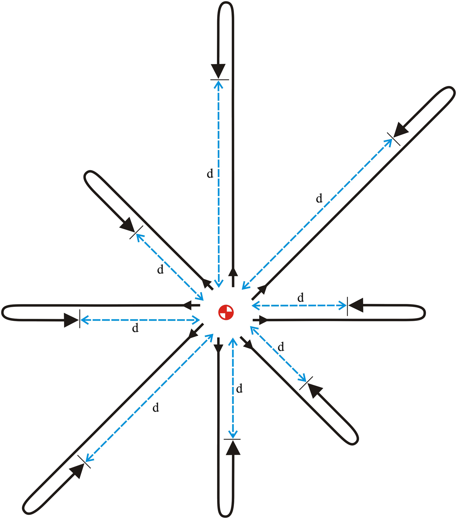
Procedure to determine range of detection (Rd).

Figure 3

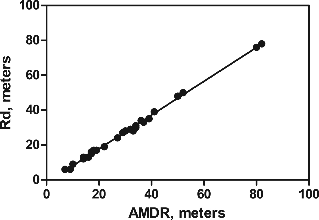
Relationship between range of detection (Rd) and average maximum detection range (AMDR).

Rd Versus W For All Search Objects

For the 27 search objects, a positive correlation was found between the Rd and the W values. The slope of the best-fit straight line with a y-intercept of 0 is 1.645 with a 95% CI of 1.475 to 1.816. The R² value is .8268. This suggests that if Rd is known, then a relationship exists that can be used to estimate the W value.

Rd Versus W By Search Visibility Class

It might be expected that more accurate Rd-to-W multipliers may be derived if each search visibility class (high-, medium-, and low-visibility) is examined individually. Indeed, in earlier experiments, placing low-visibility clues according to high-visibility AMDR values caused the vast majority of gloves not to be detected.¹³ Figure 4 shows the relationship between Rd and W for the 3 search object classes fit to individual curves. The 3 separate trend lines are all produced with a best-fit straight line with a y-intercept of 0. Table 2 summarizes the results. The high-visibility class indeed shows a better fit (higher R² value) than the pooled estimate. However, the other visibility classes are more scattered, possibly because there were fewer medium- and low-visibility search objects. An ANOVA was conducted to test the slopes of each fit: the P-value for the ANOVA is .0073 (3 groups, F = 6.081, R² = .3363), strong evidence that at least some slopes are different. A pairwise Tukey post hoc test confirms the slopes for the high- and low-visibility objects differed at the P < .01 level. The slope for the medium-visibility objects did not differ significantly from the other slopes.

Figure 4

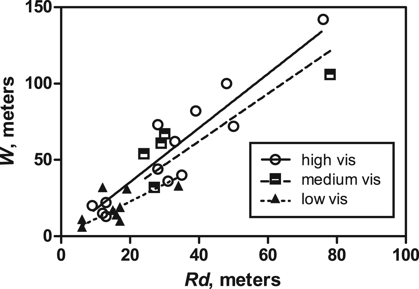
Relationships between effective sweep width (W) and range of detection (Rd) for 3 classes of visibility.

Table 2

Comparison of range of detection versus effective sweep width among the 3 visibility classes and all data combined

Variable	Combined	High visibility	Medium visibility	Low visibility
n	27	13	5	9
Slope	1.645	1.773	1.556	1.135
95% CI	1.475–1.816	1.545–2.002	1.037–2.076	0.7634–1.507
R ²	.827	.867	.560	.319

Discussion

The results of this paper provide a practical and scientific technique to estimate W for visual search in the land environment where no ESW experiment has yet been done. The positive correlation between Rd and W (R² = .83) will allow for a meaningful estimate of W in the field. This estimate could, when appropriate, be determined by search teams before performing their assigned tasks. Alternatively, the W estimation (Rd procedure) could be a task in itself, performed early in the search to acquire W values to be used in assessing later teams’ efforts. In either case, the searchers can use the simpler Rd as an excellent stand-in for the more cumbersome AMDR. (The extremely high correlation between Rd and AMDR [R² = .997] is not particularly surprising because the Rd value was already half of the measurements that comprise the AMDR process, and the Re was usually within a few meters of the Rd. In only 22% of the cases was the AMDR greater than Rd by more than 4 m. The slope of the best-fit straight line was 0.97, meaning for field purposes Rd = AMDR.)

Recommended Correction Factor(S) For Field Use

We found a correction factor of 1.645 from Rd to W to be a good overall estimate (R² = .83). In other words, if an Rd of 10 m was measured, then the estimated W would be 16.45 m. The actual value, although previously unpredicted, is not completely unexpected. The Rd value is a 1-sided value from 1 direction. In reality, a searcher will look both left and right. If measured Rd is close to the true maximum detection range, then the theoretical maximum for a correction factor for Rd is 2, but otherwise, Rd and W have no specific theoretical correlation.¹⁹ Therefore, it does make sense that we found correction factors of less than 2. Recall that the AMDR procedure uses or creates an alerted searcher, whereas the ESW experiments use unalerted searchers. While conducting AMDR measurements, the researchers never missed the search object. During the actual ESW experiments, searchers missed search objects even with lateral ranges of 0 (walking on or over a search object without detection). In fact, early research into visual detection and visibility identified factors that are related to an alerted searcher versus an unalerted searcher. These factors include improved vigilance, general knowledge of location, and knowledge of size and general time of when a detection should take place.³⁰ More recently, research on the effects of being cued (alerted) on vigilance tasks similar to visual searching have been reported.³¹ It can also be hypothesized that the unalerted searcher correction factor varies with contrast or visibility. For this reason we examined the correction factor for high-, medium-, and low-visibility search objects separately.

For the 3 different visibility classes, we found different correction factors for Rd-to-W. The correction factors for high visibility (1.773), medium visibility (1.556), and low visibility (1.135) show an appropriate relationship. It would be expected that the unalerted searcher “penalty” would be the least for a high-visibility search object and its W value would approach the theoretical limit of twice the Rd value. The low-visibility search objects would require more-focused searching and without being primed would be more difficult to detect. This is an important point regarding the psychology of visual search: the smaller multipliers for the lower-visibility color objects are not simply because of the difficulty of seeing them against the background environment. That is already accounted for in the lower Rd values for these objects. Rather, the smaller multipliers stem from the fact that these objects are less likely to be noticed by an unalerted searcher, quite apart from their lower visibility.

Although the correlation between Rd and W was relatively strong for the high-visibility class (R² = .87), it was less so for the medium-visibility (R² = .56) and low-visibility (R² = .32) classes. There are a number of possible reasons, chiefly sample size and intrinsic variability. Although the high-visibility value was based on a count of 13, the medium-visibility (n = 5) and low-visibility (n = 9) values derived from smaller samples. Additional experiments could help improve the R² values. The medium-visibility (dark blue) search objects presented more variability. In some environments and under some light conditions they were more visible, while under other conditions they could be difficult to visualize.

Only the difference between the high- and low-visibility correction factor (slope) was statistically significant. This might have been caused by the limited number of experiments involving medium-visibility search objects. If this is in fact the case, then the best solution is to conduct additional experiments with medium-visibility search objects.

Although our results have shown fairly robust evidence of a difference in correction factor between high- and low-visibility objects, it should be noted that the standard deviations of these measurements are still fairly large compared with the measurements—ranging from about 25% to nearly 50%. Therefore, at this time these figures should not be used with more than 2 significant digits.

Although the overall correction factor, 1.6, could possibly be used, our data indicate that it probably supplies an overly optimistic POD for low-visibility objects, and therefore may not be the best choice. Preferably, operational correction factors for high- and low-visibility objects should be 1.8 and 1.1, respectively. Our data do not currently indicate a significant difference between the medium-visibility and other objects; with caution, the measured value of 1.6 (which, interestingly, is the same as the overall value) may be used. However, a more conservative approach would be to use the low-visibility value of 1.1 for medium-visibility objects.

Operational Significance of the 95% Confidence Interval

In this section we show that under plausible search assignments, the uncertainty in our estimates corresponds to about an 8% difference in estimated POD. This is a substantial improvement on the 60% uncertainty in subjective estimates. Recall that ultimately W has no purpose other than to calculate a POD. (W is not to be confused with tactical spacing between searchers. In general it has no relationship to spacing. There are special cases in which a relationship may be found, subject to certain assumptions and constraints.) Therefore, we calculate the variation in POD between the lower and upper W estimates, using plausible operational assumptions.

Assume for the sake of comparison that the size of the search area is 1 km² and a team of 9 searches the area completely and expends sufficient effort to obtain a total trackline length (TTL) of 45,000 m (5 passes × 1,000 m × 9 searchers). With an Rd value of 20 m, the estimated W = 20 m × 1.645 = 32.9 m; using the exponential detection function, the POD value obtained will be 77%.

If we replace the correction factor of 1.645 with the lower bound value of 1.475 (estimated W = 20 m × 1.475 = 29.5 m), the calculated POD value becomes 73%. If the upper bound of 1.816 is used (estimated W = 20 m × 1.816 = 36.3 m), then the calculated POD value becomes 80%. Therefore, for a typical SAR scenario, the difference in POD between using the bottom (73%) and the top (80%) of the 95% range for the slope of the regression is less than 10%. This small difference would not likely be operationally significant in a higher coverage scenario. If we reduce coverage to 3 passes, the difference is still only 8% (lower bound 54%, upper bound 62%). The impact would be greater at even smaller coverage, but smaller coverage often means searchers are no longer in sight of each other, and this tactic is often avoided for safety reasons.

AMDR, Rd, AND Re

It is important to recall that the AMDR (and hence Rd and Re) measurements were taken by researchers separate from the actual ESW experiments, and that the researchers knew beforehand where the search objects being assessed were located. By comparison with the ESW experiment itself, in which object locations were randomized and the searchers did not know where to look, the researcher was always alerted (cued) to the relative position, shape, and color of the search object. In addition, during the 8 legs of the AMDR process, the researchers would notice and learn local landmarks that would assist in detecting the object. Therefore, it is not surprising that even for the low-visibility search objects only small differences existed between Rd and Re.

For searchers in the field who wish to estimate W, the Rd value will be sufficient. Because searchers would continue to walk toward the search object after making the detection, they can use their pace count (already part of field training) to determine the distance.³²

The AMDR procedure is, however, more exacting, and may still be appropriate for calibrating ESW experiments. However, we have seen that it has the same correlation with W as does Rd, so would be unjustified in field operations.

We recommend searchers adopt an 8-point field estimate of detectability (Rd procedure as shown in Figure 2), and use that to estimate W and then estimate POD as described in this paper, to wit, as a function of coverage. This is far more objective and defensible than having search teams subjectively estimate POD directly by introspection.

General Discussion

In this paper, we suggest a relationship exists between Rd and W. We have described the strength of the relationship as a correlation. However, this is merely an empirical correlation—we do not yet know the theoretical relationship, and a linear model may be incorrect. Nevertheless, the robustness of the empirical relationship and the far simpler method of measuring Rd suggest an important operational role for using Rd to estimate W.

An AMDR or Rd measurement only considers environmental factors for the relatively small area it encompasses, whereas an ESW experiment integrates the entire track. Nevertheless, the data suggest it is still possible to estimate the much more inclusive W value from the relatively small area used during the AMDR or Rd process. During actual search incidents, a search team may encounter highly variable terrain within its assigned search area. It is suggested in these circumstances that teams conduct Rd measurements as needed to reflect the conditions encountered.

Limitations and Further Work

Although the 10 experiments were conducted in 6 different ecoregion provinces and in flat, hilly, and mountainous terrain, all but 1 of the experiments were conducted in the humid temperate domain. Therefore, the correction factor may have a potential bias.

The results describe empirical field results. It provides no explanation for what is causing the results. It can be hypothesized that differences may be related to an alerted and unalerted searcher or differences in searching technique. Searchers approach the search object straight-on while conducting an AMDR or Rd procedure. On actual searches and during the ESW experiments, most of the detections occurred while looking to the side (2–4 o’clock and 8–10 o’clock).

W is a complex product of the nature of the search object (size and contrast), the searcher (visual searching and cogitation), and the environment in between the 2. Maritime W tables allow the user to look up W based on the type and size of search object (person in the water, life raft, etc.), search platform (helicopter, aircraft, ship, platform altitude, etc.), and environment (visibility, wind, seas). For the land search, it is hypothesized (but incompletely tested) that the critical factors might be type of search object (size and visibility), search sensor (ground searcher, dog team, mounted team, etc.), and the environment. The land environment is far more complex and variable than the maritime environment; however, critical factors may be the density of vertical obstructions, the height of ground cover, and the density of ground obstructions such as logs and rocks. Future work along these lines strictly tied to ESW experiments would be difficult and time-intensive. However, if an Rd measurement can be used as a proxy for W, it might be possible to conduct the types of experiments on land that can lead to the development of tables like the maritime W tables. In addition, as we have noted, Rd measurements can be used to provide a quick estimate for environments for which W values are not yet available. In the future this will allow for experiments to look at factors (via remote sensing) that may prospectively predict putative W values before resources are placed into the field. A prospective W allows for planners to use search per unit of time.⁷

Recommendations for Searchers

It is suggested that searchers and search planners can start using the correction factors at this time. While in terrain representative of their assigned search area, the team should place an object representative of the objective of the search effort. In most cases this will be something human-sized displaying the same visibility class the subject is believed to be wearing. The Rd measurement should be conducted (as shown in Figure 2) taking the mean of the 8 different legs. Searchers may pace the distance from where they make the detection to the actual test object (which might be another team member). If searchers encounter significantly different terrain within their assigned area, they can repeat the procedure.

Neither the Rd value nor the W value has any particular tactical significance. Instead it is used for calculating the POD. In fact, unless searchers extend their visual searching beyond W, they will almost certainly achieve a smaller W. In addition, if searchers need to spend additional effort to investigate areas of interest or see around obstructions, this extra effort will be captured by the total trackline length and increase the POD value accordingly. Search teams only need to report the Rd distance, the number of searchers, and a trackline distance (obtained by a GPS receiver odometer or estimated from time searching and team velocity). Search management can then estimate the POD using formal search theory as shown in Table 3.

Table 3

Measurements and calculations required to determine the probability of detection

Letter	Term	Units	How obtained/derived
Rd	Range of detection	Length	Obtained in field
W	Sweep width	Length	W = Rd × Cf (correction factor)
			Cf = 1.1 low-visibility class
			Cf = 1.6 medium-visibility class
			Cf = 1.8 high-visibility class
TL	Track line	Length	TL = time searching × velocity
			or
			Measured by GPS/GNSS odometer
TTL	Total track line	Length	TTL = TL × n (number of searchers on team)
Z	Area effectively swept	Area	Z = TTL × W
A	Area	Area	Measured from map or from GIS
C	Coverage	No unit	C = Z/A
POD	Probability of detection	Percentage	POD = 1 – e^–C

Conclusions

This paper shows it is possible to derive a correction factor that allows one to estimate W from 8 field measurements of the Rd. This correction factor is based on 10 experiments conducted across North America in different types of terrain with 3 different research teams using the same methodology. Determining the Rd with a 4-person search team would take about 5 minutes. Determining W through an experiment requires typically over 200 hours and considerable planning. The latter expense in time and personnel has proved the greatest hurdle to the meaningful use of ESW on actual incidents. Although additional work remains, especially in the dryer ecoregions, it is suggested that search planners can start using the correction factor of 1.8 for high-visibility, 1.6 for medium-visibility, and 1.1 for low-visibility search objects at this time.

Footnotes

Acknowledgments

The authors wish to thank the US National Search and Rescue Committee and their member agencies for supporting this project. It would not have been possible without the Committee’s assistance and commitment, especially for the first 6 experiments.

The authors also wish to express their gratitude to all of the people and organizations that helped sponsor the 10 experiments. During the Shenandoah National Park (Virginia) experiment, a great debt is owed to Clayton Jordan (NPS), the National Park Service, the Virginia Department of Emergency Management, the Appalachian Search & Rescue Conference, and the Virginia Search and Rescue Council. The Lincoln National Forest (New Mexico) experiment would not have been possible without Mike Lowe and Bob Rogers, who helped plan the New Mexico Escape Event. The entire staff of National Association for Search and Rescue (NASAR) made the Lansdowne (Virginia) experiment held at the NASAR Response Conference possible. For the Gifford National Forest experiment held in Washington State, thanks to Gene Seiber of the Lewis County Sheriff’s Office and Chris Long of the Washington Emergency Management Division for their hard work and support. Without Chris Young of the Contra Costa County Sheriff’s Office Search and Rescue Team and the Bay Area Search and Rescue Council, the Mt Diablo State Park (California) experiment could not have occurred. The Manheim experiment (Pennsylvania) was undertaken under the auspices and with the help of the Pennsylvania Search and Rescue Council, at their SAR-Ex conference. Similarly, the 3 experiments at State Game Lands 203 were made possible by the permission and ongoing assistance of the Pennsylvania Game Commission. The Mt Greylock “Detection in the Berkshires” experiment (Massachusetts) was conceived and organized by Richard Toman (then of Massachusetts State Police) and Daniel O’Connor. Searchers and base staff were provided by the Chicopee Civil Air Patrol under Major Dawn Tardiff. Environmental Police Officer John Tranghese took care of many little and some large logistics issues, ensuring everyone was where they needed to be. Trail access and on-site lodging was facilitated by Department of Environmental Conservation Ranger Bob Rando. Clues were provided by New Balance. Kenneth Hill, David Perkins, and Pete Roberts provided valuable assistance and (sometimes bemused) input.

Last, but certainly not least, the heartfelt gratitude and sincere appreciation of the entire experiment team is extended to all those volunteers and teams—too numerous to name here—who took time from their activities during each of the experiments to participate in the experiments. Their participation not only produced the needed data, it also produced many useful and relevant comments, suggestions, and observations.

☆

Source of support: The first 5 experiments were supported by contract DTCG32-02-D-R00010 from the US Coast Guard. The final development of IDEA was supported by contract HSCG32-04-D-R00005 from the US Coast Guard and the Manheim experiment was partially supported (some personnel and equipment). The Mt. Greylock experiment was partially supported by the Massachusetts State Police and Department of Environmental Conservation (personnel and equipment); visibility clues were donated by New Balance. The Pennsylvania experiments received financial support for equipment and supplies from the Allegheny Mountain Rescue Group. Thanks also go to GraphPad for donating its Prism software package to Allegheny Mountain Rescue Group.

References

Koopman BO. Search and Screening. OEG Report No 56. Alexandria, VA: Center for Naval Analyses; 1946http://www.cna.org/sites/default/files/research/1100005600.pdf. Accessed November 5, 2013..

Koopman BO. Search and Screening: General Principles With Historical Applications. Rev. ed. New York, NY: Pergamon Press; 1980.

Charnes

Cooper

W.W.

The theory of search: optimum distribution of search effort. Manage Sci 1958; 5, 44–50.

Frost

J.R.

Principles of search theory, part I: detection. Response 1999; 17, 1–7.

Frost

J.R.

Principles of search theory, part II: effort, coverage, and POD. Response 1999; 17, 8–15.

Frost

J.R.

Principles of search theory, part III: probability density distributions. Response 1999; 17, 1–10.

Frost

J.R.

Principles of search theory, part IV: optimal effort allocation. Response 1999; 17, 11–23.

Syrotuck

W.G.

Analysis of Lost Person Behavior . Mechanicsburg, PA: Barkleigh Productions, 1975.

Koester

R.J.

Stooksbury

D.E.

Behavioral profile of possible Alzheimer’s disease patients in Virginia search and rescue incidents. Wilderness Environ Med 1995; 6, 34–43.

10.

Koester

R.J.

Lost Person Behavior: A Search and Rescue Guide on Where to Look—for Land, Air, and Water . Charlottesville, VA: dbS Productions, 2008.

11.

Lin

Goodrich

M.A.

A Bayesian approach to modeling lost person behaviors based on terrain features in wilderness search and rescue. Comput Math Organ Theory 2010; 16, 300–323.

12.

Twardy CR, Jones N, Goodrich M, et al. MapScore: a portal for scoring probability maps. Paper presented at: Military Operations Research Society Symposium, June 2012; Colorado Springs, CO..

13.

Chiacchia

K.B.

Houlahan

H.E.

Effectors of visual search efficacy on the Allegheny Plateau. Wilderness Environ Med 2010; 21, 188–201.

14.

Koester

R.J.

Cooper

D.C.

Frost

J.R.

Robe

R.Q.

Sweep Width Estimation for Ground Search and Rescue . Washington, DC: US Dept of Homeland Security, US Coast Guard Operations (G-OPR), 2004.

15.

Cooper

D.C.

Frost

J.R.

Robe

R.Q.

Compatibility of Land SAR Procedures With Search Theory . Washington, DC: US Coast Guard Operations (G-OPR), 2003.

16.

Stone

L.D.

Theory of Optimal Search . 2nd ed Catonsville, MD: INFORMS, 2004.

17.

International Maritime Organization and International Civil Aviation Organization (IMO/ICAO). International Aeronautical and Maritime Search and Rescue Manual. Vol II. Mission Co-ordination. London/Montreal: International Maritime Organization (IMO) and the International Civil Aviation Organization (ICAO); 2010..

18.

Edwards

N.C.

Jr Mazour

T.J.

Hover

G.L.

Osmer

S.R.

Factors Affecting Coast Guard SAR Unit Visual Detection Performance . Washington DC: US Coast Guard, Office of Research and Development, 1981.

19.

Robe

R.Q.

Frost

J.R.

A Method for Determining Effective Sweep Widths for Land Searches: Procedures for Conducting Detection Experiments . Alexandria, VA: Potomac Management Group, 2002.

20.

Bailey

R.G.

Description of the Ecoregions of the United States. 2nd ed revised and expanded, Misc Publ No 1391 . Washington DC: US Dept of Agriculture, Forest Service, 1995.

21.

McNab

W.H.

Cleland

D.T.

Freeouf

J.A.

Keys

J.E.

Jr Nowacki

G.J.

Carpenter

C.A.

Description of “Ecological Subregions: Sections of the Conterminous United States.” . Washington, DC: US Dept of Agriculture, Forest Service, 2005.

22.

Fry

Xian

Jin

et al. Completion of the 2006 National Land Cover Database for the Conterminous United States. Photogrammetric Eng Remote Sensing 2011; 77, 858–864.

23.

Wartes

An Experimental Analysis of Grid Sweep Searching . Sunnyvale, CA: Western Region Explorer Search and Rescue (ESAR), 1974.

24.

Perkins

Critical Separation: Its Role in Search Management in Theory and Practice. In: LaValla

ed. Probability of Detection (POD) Research and Other Concepts for Search Management . Olympia, WA: Emergency Response Institute, 1989.

25.

Wartes J. Letter to the Editor. Response. April/May 2005:25..

26.

Cooper

D.C.

Frost

J.R.

Selected Inland Search Definitions . Olympia WA: DC Cooper, 2000.

27.

Twardy CR. Berkshires 2006 Sweep Width Experiment. SARBayes. 2013. Available at: http://sarbayes.org/search-theory/berkshires-2006-sweep-width/. Accessed December 4, 2013.

28.

Koester

R.J.

Guerra

Frost

J.R.

Cooper

D.C.

. A Simple Guide to Conducting Ground Search and Rescue Detection Experiments , Vol II. Washington DC: US Dept of Homeland Security, US Coast Guard Office of Search and Rescue (G-RPR), 2006.

29.

GraphPad Software. How does Prism compare the slopes of linear regression lines? If there are three or more lines, how can I account for multiple comparisons? GraphPad Websitehttp://www.graphpad.com/support/faqid/248. Accessed August 6, 2012..

30.

Duntley

S.Q.

Gordon

J.I.

Taylor

J.H.

et al. Visibility. Appl Opt 1964; 3, 549–598.

31.

Gunn

D.V.

Warm

J.S.

Nelson

WTBRS

Schumsky

D.A.

Corcoran

K.J.

Target acquisition with UAVs; vigilance displays and advanced cuing interfaces. Hum Factors 2005; 47, 488–497.

32.

National Association for Search and Rescue, Cooper DC, ed. Fundamentals of Search and Rescue. Sudbury, MA: Jones and Bartlett Publishers; 2005.

Use of the Visual Range of Detection to Estimate Effective Sweep Width for Land Search and Rescue Based On 10 Detection Experiments in North America

Abstract

Objective

Methods

Results

Conclusions

Keywords

Introduction

Methods

Definitions

ESW Experiments

Statistical Analysis

Results

Overall Data From All Experiments

AMDR VersusRd

Rd Versus W For All Search Objects

Rd Versus W By Search Visibility Class

Discussion

Recommended Correction Factor(S) For Field Use

Operational Significance of the 95% Confidence Interval

AMDR, Rd, AND Re

General Discussion

Limitations and Further Work

Recommendations for Searchers

Conclusions

Footnotes

Acknowledgments

☆

References