
Abstract
Background
Although lost-person search managers try to direct search efforts quantitatively, it has historically been difficult to quantify the efficacy of search efforts accurately. The effective-sweep-width (ESW) methodology represents an avenue for accomplishing this goal but has not yet been widely disseminated among practitioners.
Methods
We obtained ESW values in the summer and winter in a typical disturbed-forest environment in southwest Pennsylvania. We used nonparametric statistics to compare individual ESW values for two types of search objects detected by 18 summer and 20 winter searchers, cumulating the P values for similar comparisons and correcting for false discovery via a stepped method.
Results
We detected robust differences (all at P <.001) associated with search object color, season, and vegetation thickness. In contrast with earlier studies, we found a significant correlation between individual searchers' ESWs for different search objects and different types of vegetation (P <.001). We also found that adolescent searchers had significantly lower ESW values than adults (P = .002). Apparently significant positive correlations between time spent on the course or field search experience and ESW disappeared when teens were excluded from the comparisons.
Conclusions
These results (the first comparison of seasonal ESW effects in identical terrain) represent the first statistical demonstration that the ESW methodology provides more than enough resolution to answer fundamental questions about the efficacy of visual search for lost persons by human searchers. They also add support to the imperative of operationally disseminating these methods among search-and-rescue practitioners, and offer some initial operational lessons for search managers.
Keywords
Introduction
Lost-person searches almost always take place in the absence of fully sufficient resources to search everywhere the subject might be located. Success in the great majority of searches, therefore, hinges on efficient prioritization of limited efforts.
Usually, some portions of the search area are more likely to contain the lost person, or search subject, than others. In addition, variations in the environment within the search area often affect both the ability to detect the subject and the speed at which productive searching can be performed. Standard-of-practice methods for search and rescue (SAR) management attempt to address both of these issues in a quantitative manner. Statistics regarding lost-person behavior can help determine which portions of the search area are more likely and which are less likely to contain the subject 1 –3; reports from search-team leaders can help address the latter issue.
In planning their efforts, incident managers break the search area into a number of sub-areas called “segments” or “sectors” of manageable size for a field team to search. Then the issue becomes one of deciding how much of the available effort should be placed in each of these segments. Note that, because of limited resources, some segments initially may be left unsearched in favor of more promising segments.
One of the tools used to address the question of whether a given segment has been sufficiently searched is direct estimation of probabilities of detection (PODs, often subjectively modified by debriefing officers). 4 By definition, POD is the probability of detecting the search object, given (or assuming) that it is present and available to be detected. However, the limited data available suggest that PODs estimated by field-team leaders are almost never accurate. 5
Searches that fail do so either because all search resources were sent to the wrong places to look and there was no subject there to be detected (ie, the search area was incorrectly defined), or at least some search resources were sent to the right place to look but failed to detect the subject even though the subject was present. There seems to be ample evidence that both situations are common. However, after an initial search fails to turn up any sign of the subject, there is a tendency to assume the subject was not in the searched segments and ignore the equally valid, and probably equally or more likely second possibility (although proper SAR management training warns against this error). This tendency is exacerbated by the glaring problems with estimating PODs subjectively and argues that a better methodology for both predictive (for search-planning purposes) and retrospective (for purposes of evaluating the effectiveness of prior searching) estimation of POD values is needed immediately.
The effective-sweep-width (ESW) methodology promises a vast improvement in deriving accurate, objective PODs. ESW is the lateral distance from the searcher who defines an envelope within which the number of search objects missed inside that envelope equals the number of search objects detected outside. Via an exponential function that factors in distance walked through the area and number of searchers in the team, ESW can be used to calculate objective PODs.5,6 ESW makes it possible to establish an objective, mathematical relationship between the amount of searching effort expended in a segment and the probability of detecting the search object if it is present in the segment. These more reliable PODs can better aid the search process, by making it possible to allocate the available resources in a way that maximizes the overall probability of success (OPOS), ie, the probability of finding the subject, and minimizes the time it will take, on average, to find the subject. The probability of success (POS) for a segment is the joint probability of the subject being present in the segment and being detected if present. The former is represented by POA (probability of area, also known as POC—probability of containment). Thus, POS is the product of POD and POA. The sum of all the individual (non-normalized) POS values gives the OPOS value. 7
In order to help build the collective national library of ESW figures, record ESW data for our response area in the Commonwealth of Pennsylvania (PA), and employ statistical analysis to test for the first-time hypotheses regarding effectors of ESW, we undertook two ESW experiments in State Game Lands 203 in Marshall Township, Allegheny County, PA. Following are our results regarding the effects of search object type, season, weather, vegetation, and select individual searcher characteristics on daytime human visual ESWs.
Methods
We conducted the ESW experiment in the manner of Koester et al, 5 using the IDEA Microsoft Excel worksheet provided by R. Koester and N. Guerra to automatically generate a randomized plan for an ESW course. We deviated from the method, however, in several ways. Because of time constraints we were only able to obtain one measurement of average maximum detection radius (AMDR, a rough estimate of ESW used to calibrate the course) for the winter experiment (at site #1, 17TNE7511798716; coordinates for site #2, which was used as well in the summer experiment, were 17TNE7427798476; these and other coordinates to follow are in US National Grid, Datum NAD 83). Instead of using a spray-painted olive drab work glove for our low-visibility clue, we obtained forest-green work gloves in bulk from Tractor Supply.
In the winter experiment, because of our experience with the clue in the summer experiment (see below) and with other ESW experiments 5 in which the IDEA tool overestimated appropriate lateral distances for difficult-to-see search objects, we forced the worksheet to normalize the placement of that search object to a maximum distance of 1 × AMDR rather than the usual 1.5 × AMDR. Because one of the randomized low-visibility adult search object placements had called for a lateral distance that was a fraction of a meter, we re-randomized that search object to the least represented (in the other placements of that search object type) of 3 bins (defined as 0 to 0.333 × AMDR, 0.333 to 0.667 × AMDR, and 0.667 to 1 × AMDR) using the random number generator on a Casio FX-260 Solar calculator (Casio Computer Company, Ltd., Tokyo, Japan). Finally, in the winter experiment we made use of the post-experiment confirmation box in the search object placement worksheet to record a short description of the vegetation surrounding each search object.
The area we chose was the northern part of State Game Lands 203 in Marshall Township, PA. This venue offered a representative sampling of terrains common to our operational deployments in southwest Pennsylvania. Starting point for the course was 17TNE7407598818; total length was 3,850 m for the summer experiment and 3,650 m for the winter experiment, with the last clues placed at 3,768 m and 3,600 m, respectively.
We recorded location coordinates with a Garmin GPS map 60CSX GPS (Garmin International Inc., Olathe, KS, USA) receiver using MapSource 3.02 topographic maps on the GPS unit and Maptech Terrain Navigator 6.04 (MyTopo, Billings, MT, USA) for the desktop computer. We placed the search objects along the track at the distances stipulated by the IDEA application, using a Trumeter Measuremeter 5500E (Trumeter Company Inc. [USA], Deerfield Beach, FL, USA) measuring wheel along the track and a Nikon ProStaff Laser 440 Rangefinder (Nikon Corporation, Tokyo, Japan) laterally, or a metric-scale tape measure for distances under the rangefinder's minimum (about 10 m).
The area (ecoregion, hot continental; regime, 220) is largely second- and third-growth forest that had been used for farming as well as gas and oil drilling, and more recently has been managed for game-bird habitat via selective clear-cutting and resulting succession. The woods are dominated by a mixed maple, tulip poplar, oak, cherry, and hickory canopy common to the Allegheny Plateau, with a mid-story of spicebush and sassafras and a ground cover of ferns, May apples, and naturalized multiflora rose. Occasional stands of naturalized black raspberry bramble and Concord grape vines also dot the area. The vegetation was in full leaf for the August experiment, with full summer growth of the brambles, and completely leafless in March. General vegetation types included open woods; fields and mowed trail areas; brambles; and sapling stands, the latter being the 5- to 10-year succession vegetation after clear-cutting. While the temperatures were above freezing for the March experiment, a few small patches of snow persisted from a late snowfall the previous week.
Knowledge of the thick brambles in the area convinced us that a cross-country course would be untenable. We chose, therefore, to set the course along pre-existing trails. This approach ran the risk of an “edge effect”—the clear area of the trail and transitional vegetation at its edge might have produced significantly different sight-lines than those in the interior of the area. However, the path chosen produced sight lines, terrain, and vegetation that appeared extremely similar to those we saw in the interior. While quantifying this impression is problematic, we believe that the trail-based approach, at least in this area, would not produce seriously different ESWs than we would obtain with an overland course. Our results would certainly apply to “hasty tasks” commonly performed early in a search, along linear “travel routes” such as trails, because subjects are often found near travel routes. 3
The weather for the single day of the summer experiment (August 26, 2006) proved largely clear and sunny, with a moderate (high 10s to mid 20s °C) morning and a warm to very warm (low 30s °C) mid-day to afternoon. The two days of the winter experiment provided an unexpected opportunity to compare weather conditions: March 10, 2007, proved cold (low-single digits °C) and damp, with mist, light rain, and heavy clouds throughout, but a front brought warmer (mid- to high-single digits °C), sunny weather on March 11.
Eighteen searchers followed the summer course, consisting of 21 real and 8 virtual high-visibility-adult, 20 real and 4 virtual low-visibility-adult, and 20 real and 6 virtual low-visibility-clue search objects. Each searcher walked the course individually, accompanied by a single data logger who recorded when, and in which direction, the searcher detected (or thought he or she detected) an object, and what type and color of object. We compared suspected sightings of search objects with the known placement of the objects, counting hits when the two agreed, misses when no sighting aligned with an object, and disregarding erroneous sightings. Absolute certainty that it was a real search object was not necessary on the part of the searcher; the rule for recording a sighting was whether, in a real search, that searcher would have moved closer to confirm the object's identity.
As per Koester et al, 5 “real” search objects were the actual mannequins or clues placed; “virtual” search objects were the result of randomized placements that resulted in a search object that was invisible from the course, because of vegetation, terrain, etc. In the latter cases, we counted the randomized placement as an automatic miss, and moved the mannequin in toward the course route until it was just visible to an observer who knew where it was, recording the new lateral distance. We subsequently treated the replaced search objects in the same fashion as the randomized real objects. We placed all search objects in a horizontal position, to simulate a nonresponsive (unconscious) subject, orienting each object using a randomized compass bearing supplied by the IDEA worksheet.
When confirming the search object placements after the experiment, we found that one high-visibility-adult search object had been tampered with (slashed open and orange vest stolen) but not moved, one of the low-visibility clues had moved, and two low-visibility clues were missing. Because we discovered one data logger had told searchers to disregard the high-visibility search object without the vest, that search object was not counted for that logger and searchers for whom he had logged, as well as searchers for whom they logged data; we stopped counting hits or misses for the missing and moved gloves after their last confirmed sightings in their proper locations. The end result of the discounted search objects was 518 high-visibility-adult, 420 low-visibility-adult, and 414 low-visibility-clue detection opportunities (DOs). The crossover graph for the clue only barely crossed over, at a distance of 1 m; however, since none of our randomized hiding distances for this object were less than 1 m and most of the clues lay on the trail itself, we were not confident we had accurately bracketed this detection distance. Therefore, we excluded the clue from subsequent analyses, and will address clue detection in future experiments.
Twenty searchers (12 on day 1, 8 on day 2) walked the winter course, which consisted of 17 real and 6 virtual high-visibility-adult and 16 real and 1 virtual low-visibility-adult search objects. All of the search objects remained in position at the end of the experiment, for 460 high-visibility and 340 low-visibility DOs. See Table 1 for the data collected on individual searchers in both experiments. Note that only 3 searchers participated in both the summer and winter experiments, minimizing the possibility of a bias in the winter experiment due to searcher experience; however, this may not generally be an issue with these experiments, as Koester et al observed that searchers rapidly improve their detection and reach a plateau in efficacy in the course of a single experiment, and after only a few search objects have been detected. 5
Individual searcher data
SAR, search and rescue; n/a, not applicable; n/r, not recorded; ASRC, Appalachian Search & Rescue Conference; NASAR, National Association for Search and Rescue; AMRG, Allegheny Mountain Rescue Group; DCNR, Pennsylvania Department of Conservation and Natural Resources; CAP, Civil Air Patrol; CQ, callout qualified; FTM, field team member; FTL, field team leader; GTL, ground team leader; SARTECH I, II, search and rescue technician I or II; GSAR, ground search and rescue; DH, dog handler; MSO, managing the search operation; IC, incident commander; AC, area command authority; Search object no.1, high-visibility adult mannequin; Search object no.2, low-visibility adult mannequin; Search object no.3, low-visibility clue (glove); cloud cover, % sky covered by cloud, estimated by data logger; ESW, effective sweep width.
In all cases we calculated ESW values using the crossover graph method.5,6 In order to make statistical comparisons, we calculated ESW values for individual searchers, which previous investigators have not done. While the variance in these values undoubtedly contains a fairly large random element, the statistical tests we chose are by definition capable of distinguishing that variance from systematic variance between the groups being tested.
We used GraphPad Prism version 5.02 software to perform most of our statistical testing. We cumulated raw P values from similar comparisons using the method of Fisher. 8 All tests were nonparametric and 2-tailed. We used Microsoft Excel to create a worksheet that created graphs and performed simple calculations, including correcting P values and cumulative P values for repeated testing using the step-down Hochberg/Šidác method described by Wright 9 and the Fisher P value cumulation. We used IFA Services' online calculator to generate P values for the latter. 10 Note that while parametric statistics would have been attractive for this study—parameters such as standard deviation would be operationally useful—many of the data sets were highly non-normal and did not normalize with mathematical transformation (data not shown).
As an operational SAR team, Allegheny Mountain Rescue Group has no institutional review board or process. However, all participants in this study (or their guardians, if minors) signed safety release forms explaining the risks of outdoor activities.
Results
Search-Object Characteristics and Surroundings: Object Type
We began our study with an analysis of the effects of target type and environmental factors on individual searchers' ESW values, which can be seen in Table 1. Figure 1 shows the ESW values for each adult-mannequin search object in each experiment.
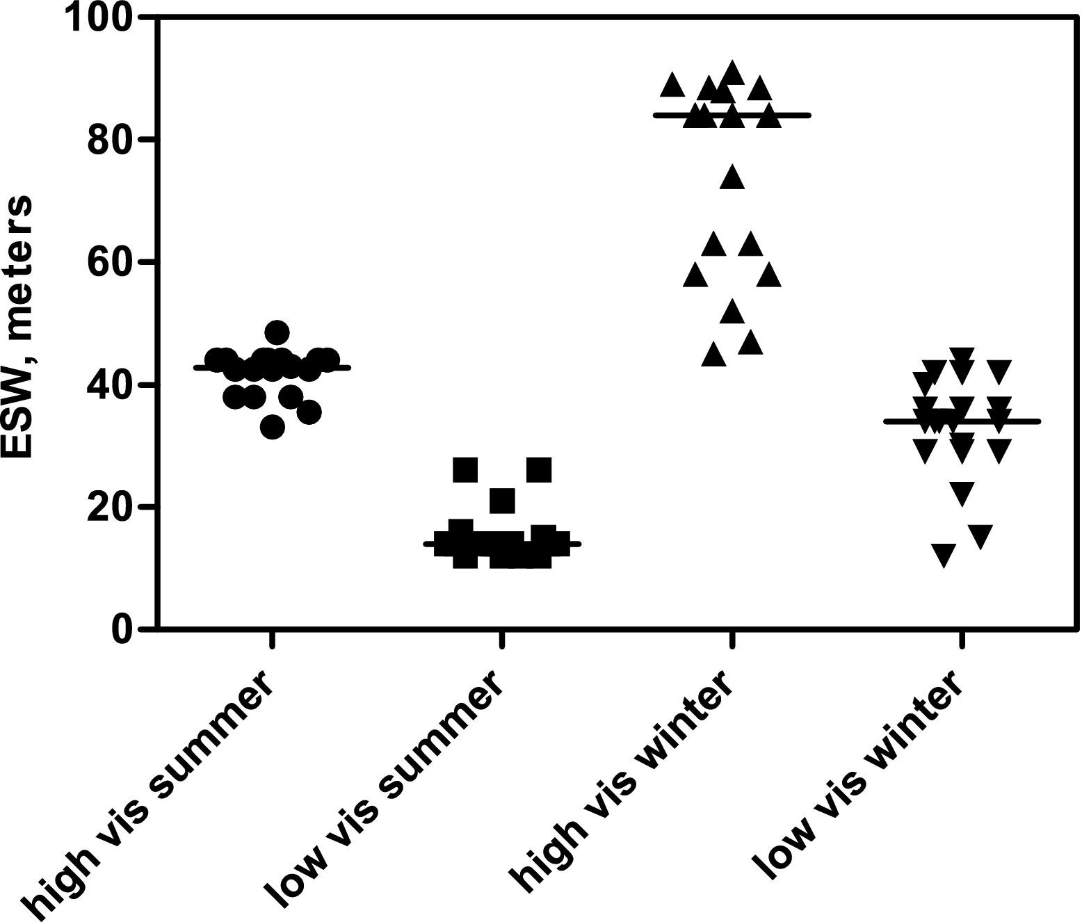
Comparison of individual effective-sweep-width (ESW) values by search-object type, either orange-and-white high-visibility adult mannequins (high vis) or olive-green low-visibility mannequins (low vis), for the summer and winter experiments. Horizontal lines show the median value for each group of data points.
We detected a highly significant difference in ESWs between the high- and low-visibility-adult search objects in both experiments. Median ESWs for high- and low-visibility search objects were 42.75 m versus 14 m, respectively, in summer (Mann-Whitney test, 11 U = 0, N1 = N2 = 18, P <.0001) and 84 m versus 34 m in winter (Mann-Whitney test, U = 0, N1 = N2 = 20, P <.0001). The corrected cumulative P value for this comparison was highly significant (Fisher P value cumulation, 8 χ2 = 36.841, df = 4, P <.001; corrected P <.001). 9
Obviously, this difference is not surprising; we would expect a white and blaze-orange search object to be more easily seen in the woods than an olive green search object. What is interesting is the fact that the relative difference between the two search objects was similar in both seasons. We might not have expected the visibility of the green search object, in particular, to be affected as greatly by the brown forest of the winter compared with the green forest of the summer, but that turned out to be the case.
Season
Perhaps the most unique aspect of the present study was our use of the same ESW course to conduct randomized experiments in two different seasons.
As can be seen in Figure 1, season had a profound effect on search-object visibility. Median values for the high visibility search object were 42.75 m versus 84 m in the summer and winter, respectively (Mann-Whitney test, U = 2, N1 = 18, N2 = 20, P <.0001), and 14 m versus 34 m for the low-visibility search object (Mann-Whitney test, U = 22.5, N1 = 18, N2 = 20, P <.0001). The corrected cumulative P value for this comparison was again highly significant (Fisher P value cumulation, χ2 = 36.841, df = 4, P <.001; corrected P <.001). What we found interesting was that the relative seasonal difference was roughly similar for both search objects, and that the rough magnitude of the color effect was similar to that of the seasonal effect.
Vegetation Thickness
The variety of vegetation in the State Game Lands 203 course, and our increasing comfort level in expanding data collection with the winter experiment, allowed us to make another operationally useful comparison in that experiment. We divided each individual searcher's data between “open” (open woods and fields) and “thick” (bramble and sapling stand) vegetation, and compared the effect of thicker vegetation on ESW. We made the judgment of what was open and what was thick while verifying search object location during disassembly of the course, and before doing any analysis of the data, so systematic bias is unlikely.
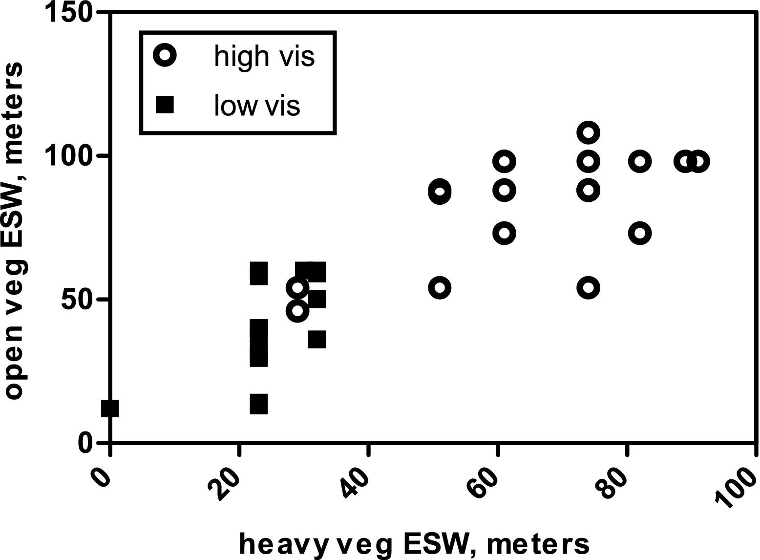
Thicker vegetation imposes a highly statistically significant penalty in ESW (Figure 2)—median ESWs for the high-visibility search object for thick and open vegetation were 74 m versus 88 m, respectively (Mann-Whitney test, U = 99, N = 20, P = .0062), and for the low-visibility search object were 23 m versus 39 m (Mann-Whitney test, U = 70, N1 = N2 = 20, P = .0003). The corrected P value of this comparison was highly significant (Fisher P value cumulation, χ2 = 26.390, df = 4, P <.001; corrected P <.001).
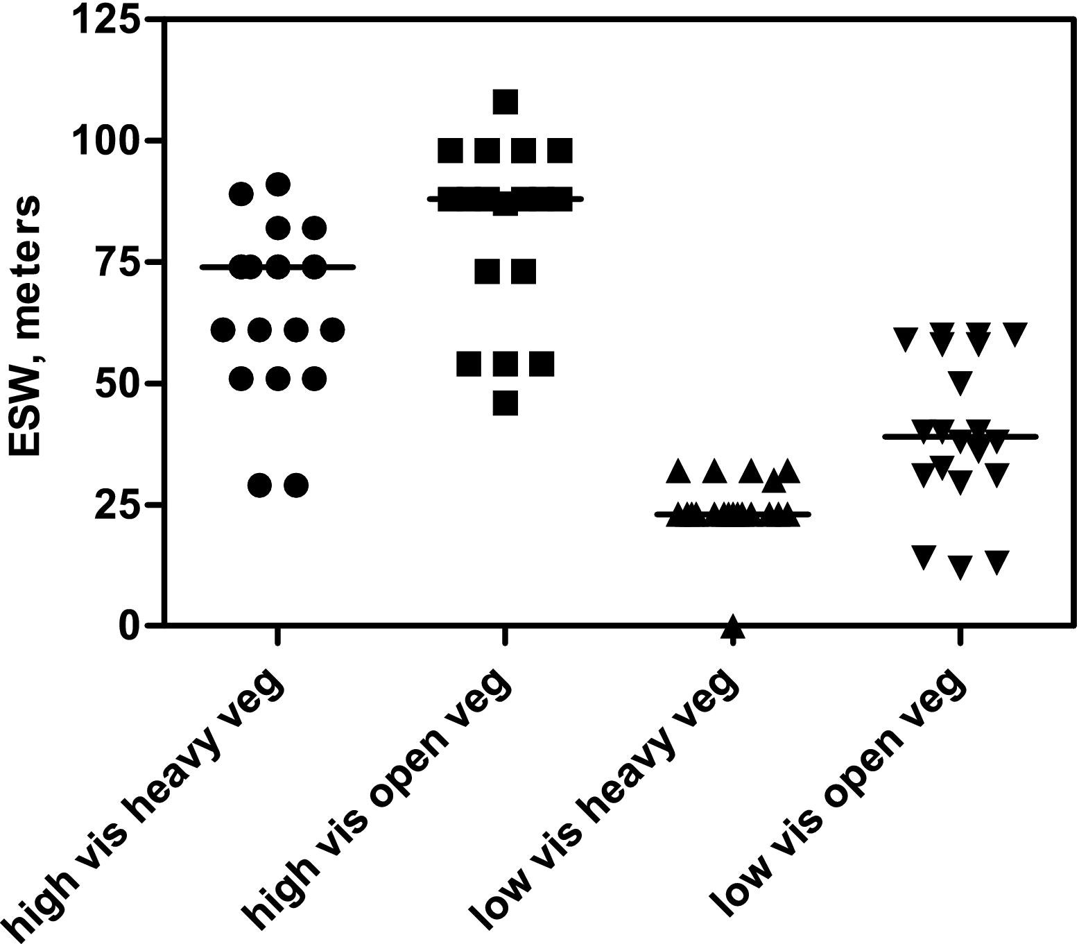
Effects of vegetation thickness on effective-sweep-width (ESW) in the winter experiment, for each search object type. High vis, high visibility adult mannequin; low vis, low-visibility adult mannequin; heavy veg, heavy vegetation; open veg, open vegetation. Horizontal lines show the median value for each group of data points.
Cloud-Cover Effects
The departure of a cold front on the second day of the winter experiment gave us an unexpected chance to compare ESWs obtained in cloudy, dim conditions (day 1) against those obtained in sunny conditions with direct light. One might expect the glare of direct sunlight to make a significant difference in visual search efficacy. As can be seen in Figure 3, median ESW values for the high-visibility search object were 84 m versus 60.5 m for cloudy versus sunny conditions, respectively (Mann-Whitney test, U = 26.5, N1 = 12, N2 = 8, P = .0975), and for the low-visibility search object were 35 m versus 31.5 m (Mann-Whitney test, U = 25, N1 = 12, N2 = 8, P = .0789). However, the cumulative P value for these differences was not significant when corrected for false discovery (Fisher P value cumulation, χ2 = 9.735, df = 4, P = .045; corrected P = .169).
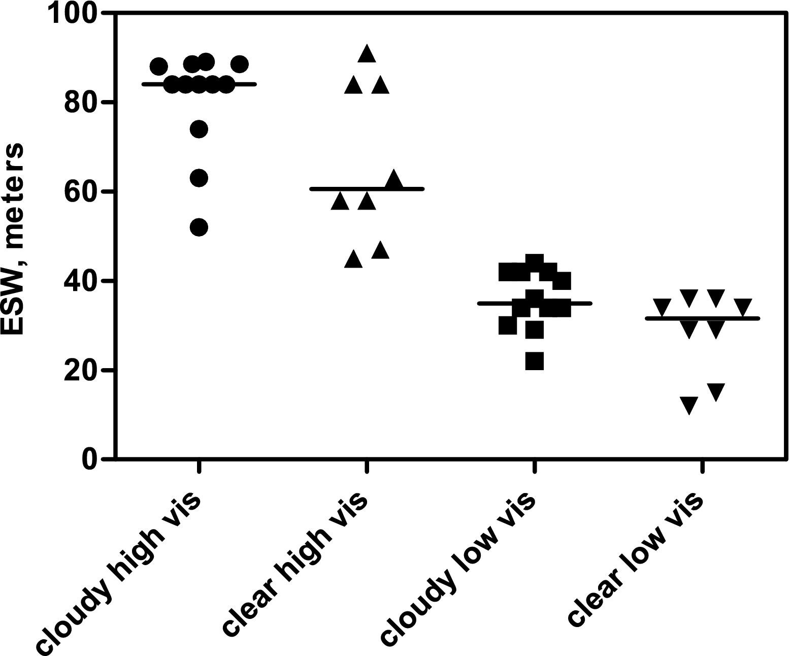
Cloud-cover effects on effective-sweep-width (ESW) for the two days of the winter experiment for each search object. Day 1 was cloudy and cold (cloudy); day two was sunny and warmer (sunny). High vis, high visibility adult mannequin; low vis, low-visibility adult mannequin. Horizontal lines show the median value for each group of data points.
Searcher Characteristics: Searcher Consistency
Figure 4 shows a comparison between each searcher's individual ESW for the high- and low-visibility-adult search objects in the summer and winter experiments. Unlike previous ESW results, 5 the State Game Lands 203 data show signs of correlation between each searcher's ESW for the high- and low-visibility search objects (white and blaze-orange vs olive-green mannequins of adult human size, respectively; Spearman rank correlations, 12 summer r = 0.7057, N = 18, P = .001; winter r = 0.5785, N = 20, P = .008).
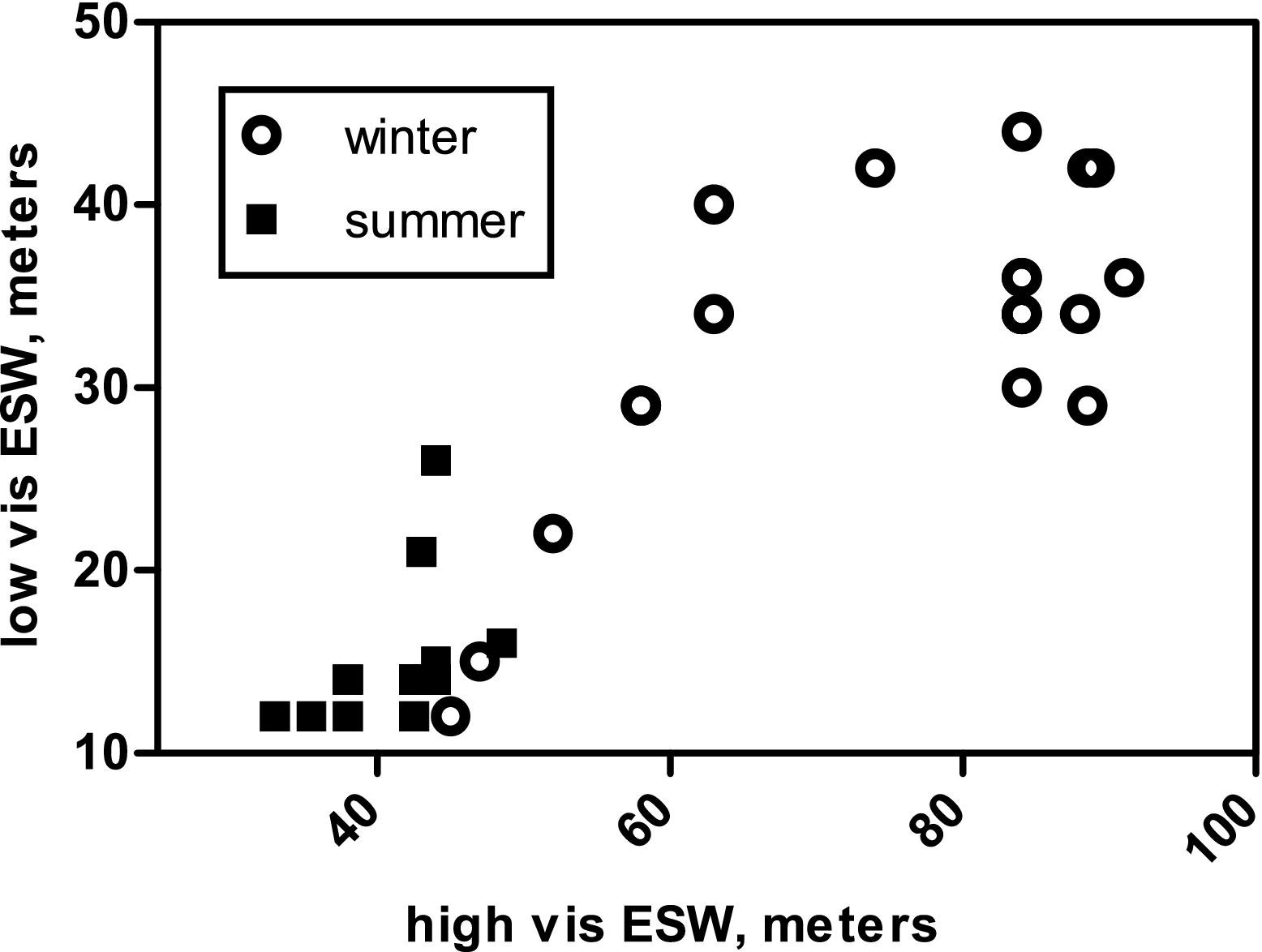
Each searcher's individual effective-sweep-width (ESW) value for the high-visibility adult search object plotted vs the value for the low-visibility (high- and low-vis, respectively) object, for each season.
Our breakdown of the winter search objects between thick and open vegetation allowed another test for searcher consistency. As can be seen in Figure 5, each searcher's open- and thick-vegetation ESWs correlated for both the high-visibility (Spearman rank correlation, r = 0.5388, N = 20, P = .014) and the low-visibility objects (Spearman rank correlation, r = 0.5524, N = 20, P = .012). The corrected P value for consistency between the two objects or between the same object in heavy or light vegetation, was highly significant (Fisher P value cumulation, χ2 = 40.833, df = 8, P <.001; corrected P <.001).
Each searcher's effective-sweep-width (ESW) value in heavy vegetation (heavy veg) vs the value in open vegetation (open veg) in the winter experiment, for each of the two search objects (high vis, high visibility adult mannequin; low vis, low-visibility adult mannequin).
We have no certain explanation as to why our results showed this relationship when earlier studies comparing detection percentages did not; see the Discussion for our speculations on this issue.
SAR Experience
We analyzed the searchers' ESW values for effects of individual characteristics. One of the more interesting issues is whether prior training or experience in SAR enables searchers to search more effectively, thus increasing their ESWs compared with untrained members of the public. The SAR community has in some quarters reacted with surprise to earlier findings that experience seems to have no effect in improving visual searching. 5
As can be seen in Figure 6, the mere presence of any national or state-sanctioned SAR certification—which we used as a stand-in for basic training in search technique, and which is the emerging standard of practice for team members to field on real searches—does not associate with higher ESW values for any of the targets in any season. Median ESW values were 44 m for the certified searchers for the high-visibility summer object versus 42.5 m for noncertified searchers for the same target/season; 14 m versus 14 m for the low-visibility summer object; 88.5 m versus 84 m for high-visibility winter; and 42 m versus 34 m for low-visibility winter. The individual comparisons missed statistical significance, (Mann-Whitney test, U = 24, 21.5, 16, and 17; N1/N2 = 7/11, 7/11, 5/15, and 5/15; P = .188, .108, .061, and .077), and so did the cumulative corrected P value (Fisher P value cumulation, χ2 = 18.510, df = 8, P = .018; corrected P = .102).
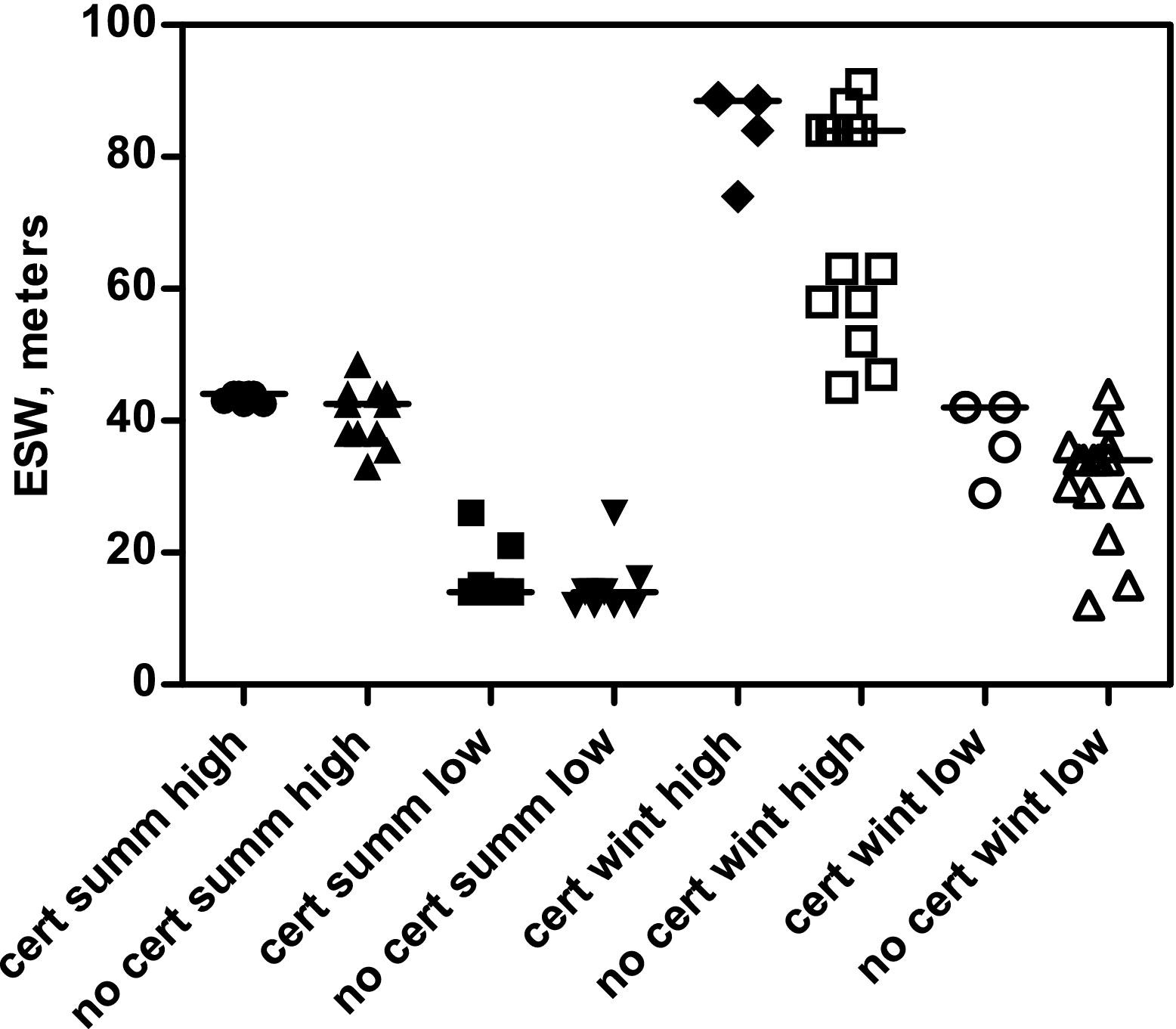
Effect of previous search and rescue (SAR) training or its lack on individual effective-sweep-width (ESW) values for each object and season. Cert, SAR-certified searchers; no cert, uncertified searchers; summ, summer; wint, winter; high, high visibility adult mannequin; low, low-visibility adult mannequin. Horizontal lines show the median value for each group of data points.
One other experiential comparison of interest to us was whether there is a statistical correlation between actual field experience—as measured by number of searches in which each searcher participated in a field, as opposed to command post, task (See Figure 7). In this case, we detected a marginal effect of experience for individual search objects/seasons (Spearman rank correlation, r = 0.1973, 0.4087, 0.4153, 0.5996, ordered as above; N = 18, 18, 20, 20; P = .433, .092, .069, .005) that was significant in cumulation (Fisher P value cumulation, χ2 = 22.321, df = 8, P = 0.004; corrected P = .030).
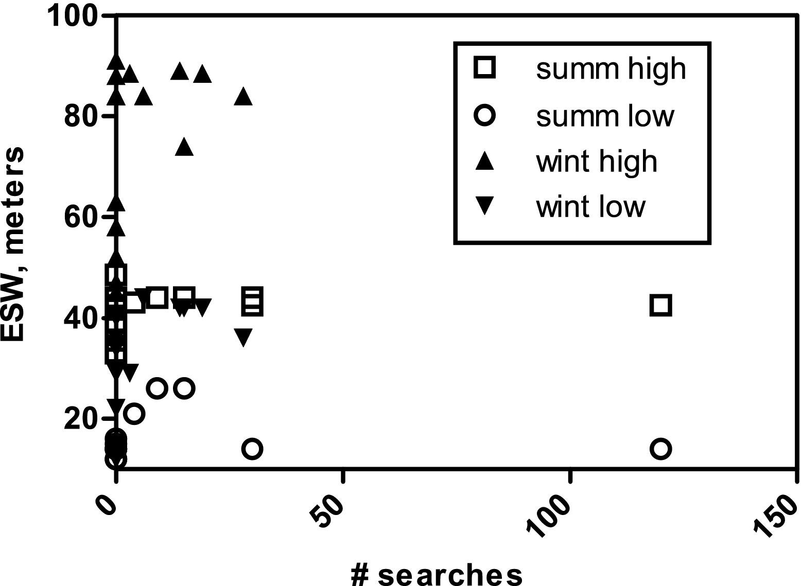
Individual effective-sweep-width (ESW) values vs search and rescue (SAR) experience as measured by number of searches deployed in the field. Summ, summer; wint, winter; high, high visibility adult mannequin; low, low-visibility adult mannequin.
Searcher Sex
From time to time it has been posited that, since red/green insensitivity is more common among men than women, sex-linked differences in the ability to carry out visual search may exist. For this reason, we compared male and female searchers' ESW values. Because we might therefore expect a differential effect on detection of targets of different color, in this case we cumulated the effects of searcher sex on the high- and low-visibility targets separately.
In neither case did we observe a significant effect of searcher sex (see Figure 8). For high-visibility/summer and high-visibility/winter, respectively, medians for women versus men were 38 m versus 44 m and 84 m versus 84 m (Mann-Whitney test, U = 16.5 and 17, N1/N2 = 5/13 and 6/15; P = .113 and .833); for low-visibility summer and winter, medians were 14 m versus 14 m and 35 m versus 34 m (Mann-Whitney test, U = 39 and 35, N1/N2 = 5/13 and 6/15; P = .112 and .587). The cumulative corrected P value was not significant (Fisher P value cumulation for the high- and low-visibility targets, respectively, χ2 = 4.732, 5.441; df = 4, 4; P = .316, .245; corrected P = .316, .570). While color perception may well have a significant effect on individual ESW values for different colored objects, clearly any sex difference is too small to be detected by an experiment of this size.
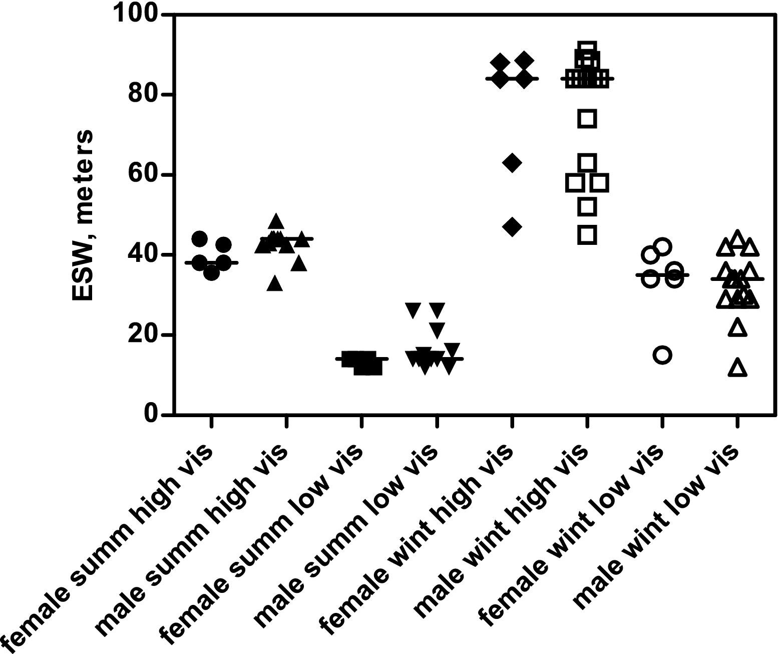
Effect of searcher sex on effective-sweep-width (ESW) values for each object and season. Summ, summer; wint, winter; high vis, high visibility adult mannequin; low vis, low-visibility adult mannequin. Horizontal lines show the median value for each group of data points.
Searching Speed
Another searcher characteristic we chose to examine was the amount of time each individual searcher took to complete the course. It seems quite probable that the searchers who took the least time to finish the course may have been rushing through it and therefore searching less effectively. However, this does not necessarily suggest that the slowest searchers are searching the most effectively. We chose, therefore, to analyze the correlation between time on the course and ESW.
In fact, we did observe a general negative correlation between time and ESW values (Figure 9; for the high-visibility/summer, low-visibility/summer, high-visibility/winter, and low-visibility/winter comparisons, respectively, Spearman rank correlation, r = 0.4166, 0.5071, 0.5769, and 0.7152; N = 18, 18, 20, and 20; P = .086, .032, .008, and <.001). The cumulative comparison was highly significant even after false-discovery correction (Fisher P value, χ2 = 37.203, df = 8, P <.001; corrected P <.001).
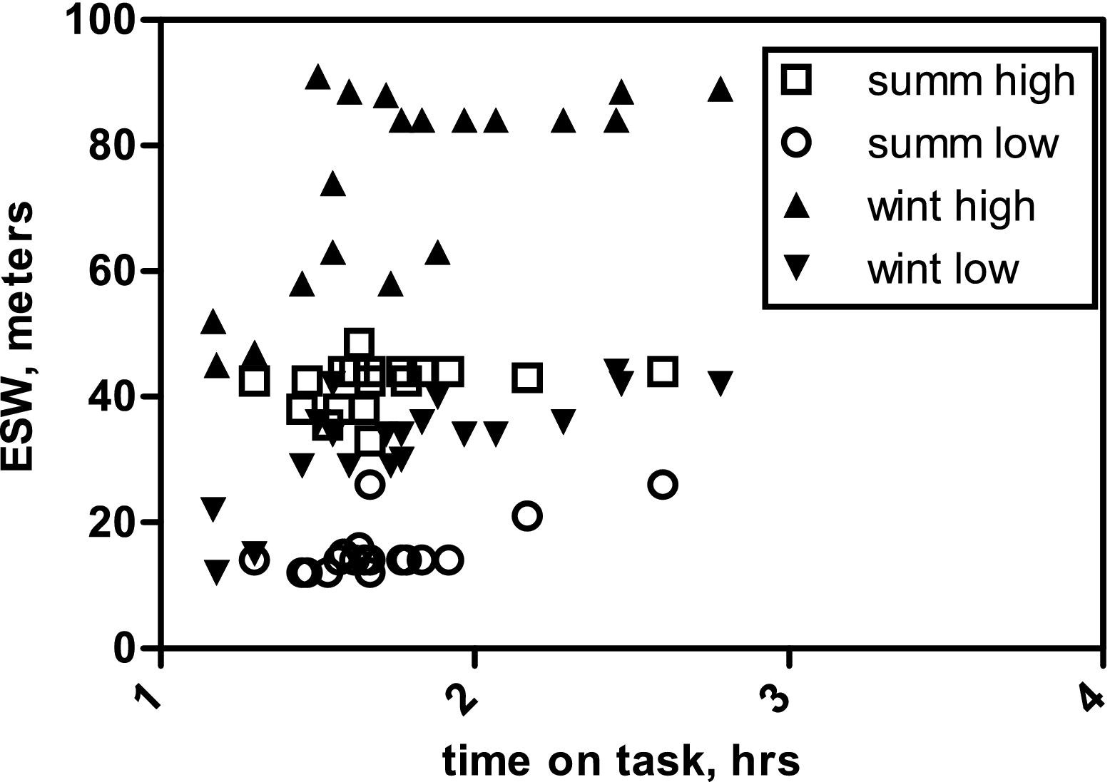
Individual effective-sweep-width (ESW) values vs time taken to complete the course for each season. Summ, summer; wint, winter; high, high visibility adult mannequin; low, low-visibility adult mannequin.
Searcher Age
Previous investigators have reported a complex apparent effect of age on individual searcher efficacy, with a concave-downward plot of percentage of objects detected versus age—the youngest searchers displaying the lowest probabilities, the oldest somewhat higher but still lower than those of searchers in the middle of the age range. 5 We decided to repeat these comparisons using our ESW values, as well as to undertake a dissection of the apparently stronger effect at the lower ages.
In our initial analysis, we examined searcher age versus ESW for each search object and season (Figure 10). Not surprisingly given the complex relationship observed earlier, we found no significant correlation using data from all of our searchers (again, the order is high-visibility/summer, low-visibility/summer, high-visibility/winter, low-visibility/winter: Spearman rank correlation, r = 0.3383, 0.3598, 0.1977, and 0.2516; N = 17, 17, 20, and 20; P = .184, .156, .404, and .285). The cumulative comparison was not significant (Fisher P value cumulation, χ2 = 9.968, df = 8, P = .267; corrected P = .463). Note that the N values for the summer experiment in this case were reduced by one because we did not have an exact age recorded for a teen member of the youth group that volunteered to walk the course.
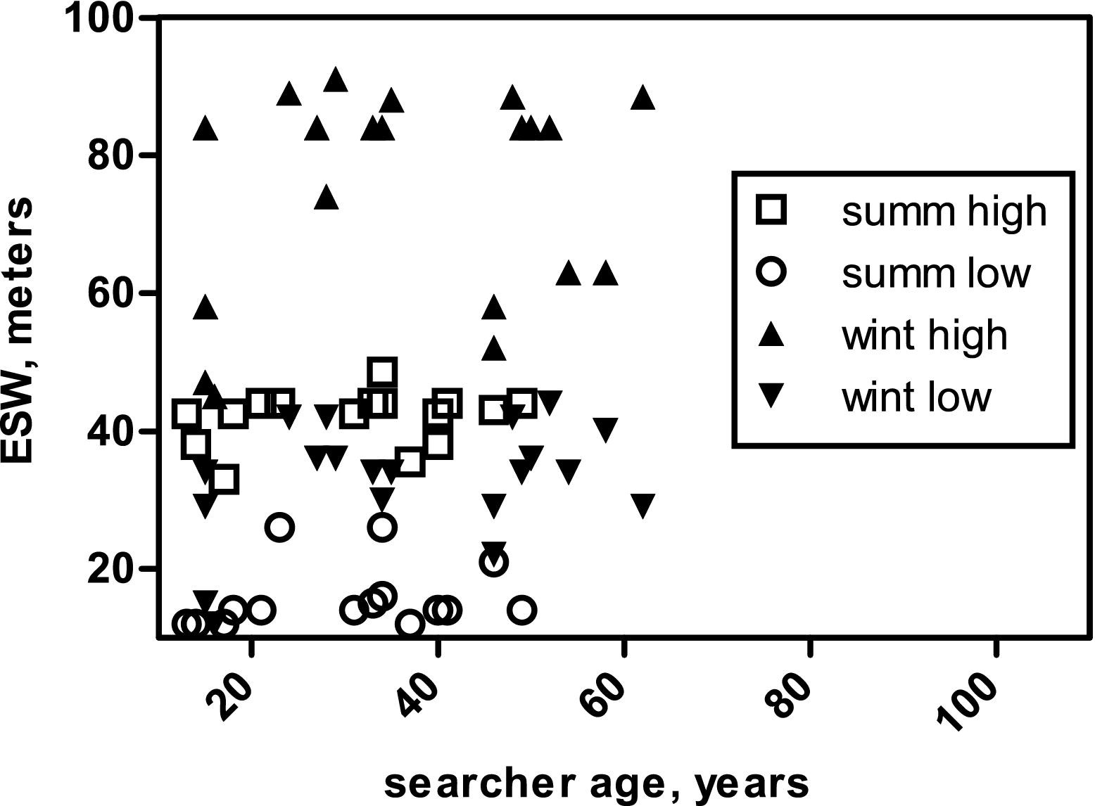
Individual effective-sweep-width (ESW) values vs searcher age in years. Summ, summer; wint, winter; high, high visibility adult mannequin; low, low-visibility adult mannequin.
A wealth of research has documented that adolescents can perform at an adult level of attention but only imperfectly. 13 Because of the common use of adolescent searchers, through the Civil Air Patrol cadet corps, Scout Explorer posts that specialize in SAR, and other similar groups, we decided to take a closer look at the divide between teen-aged searchers in our experiments and those age 20 and above.
The comparison of teen versus adult searchers demonstrated a varying but significant advantage to the older searchers (Figure 11). Median adult versus teen ESWs, in the same object/season order as previously, were 44 m versus 38 m, 14 m versus 12 m, 84 m versus 52.5 m, and 35 m versus 22 m (Mann-Whitney test, U = 9, 10.5, 9.5, 8; N1/N2 = 13/5, 13/5, 16/4, and 16/4; P = .019, .023, .034, and .025; Fisher P value cumulation, χ2 = 29.734, df = 8, P <.001; corrected P = .002).
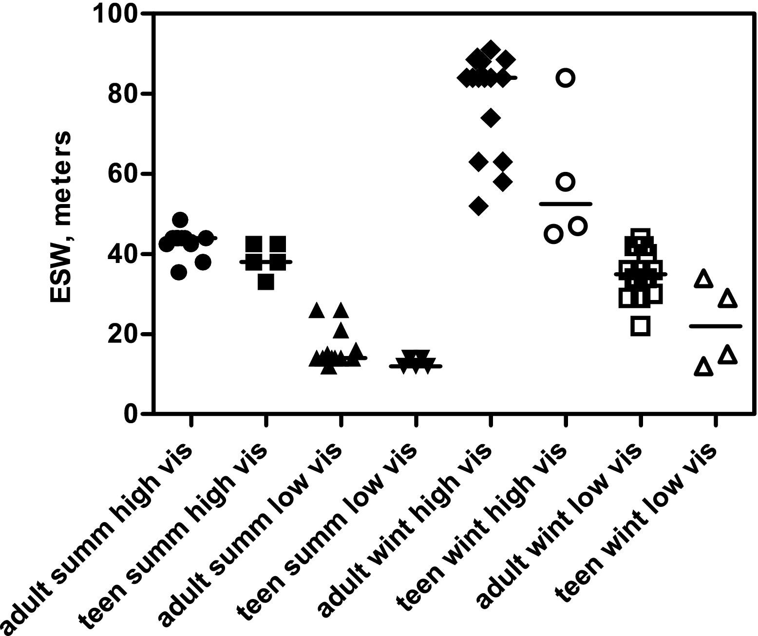
Effect of teen vs adult status on effective-sweep-width (ESW) values for each object and season. Summ, summer; wint, winter; high vis, high visibility adult mannequin; low vis, low-visibility adult mannequin. Horizontal lines show the median value for each group of data points.
This relationship between adolescence and lower ESW values posed a problem; in a number of the comparisons above, the teen searchers seemed disproportionately represented in one group or another. In order to gauge the significance of any effect of teen searchers, therefore, we re-analyzed all of our data with the teens excluded. For most of the comparisons above, this did not change the significance (or lack) of each. The exceptions were the comparisons involving SAR field experience and the relationship between time on course and ESW.
In the case of the correlation between experience as measured by number of field searches and ESW, the significance disappeared once the teens were excluded (Spearman rank correlation, r = –.1873, 0.1857, 0.3267, and 0.5887; N = 13, 13, 16, and 16; P = .540, .544, .217, and .016; Fisher P value cumulation, χ2 = 13.729, df = 8, P = .089; corrected P = .429). Since none of the teens in these experiments had any previous search experience, their lower ESW values may have skewed the result.
Another interesting change involved time versus ESW for each object/season. Although this comparison, with the teens included, was one of the strongest we observed (P <.001), removal of the teens produced a large increase in P-values (Spearman rank correlation, r = –0.2801, 0.4149, 0.3097, and 0.5766; N = 13, 13, 16, and 16; P = .354, .159, .243, and .019; Fisher P value cumulation, χ2 = 16.473, df = 8, P = .036; corrected P = .227).
To attempt more insight into this problem, we analyzed the times taken on the course for teen and adult searchers (Figure 12). We found that, while the teens did tend to finish the course more quickly than the adults, with adult versus teen median times for the summer and winter experiments, respectively, of 1.67 hours versus 1.47 hours and 1.77 hours versus 1.38 hours, these differences were not statistically significant when corrected for false discovery (Mann-Whitney test, U = 11 and 14, N1/N2 = 13/5 and 16/4, P = .038 and .098; Fisher P value cumulation, χ2 = 11.181, df = 4, P = .025; corrected P = .117 or .181 in the stepped correction including or excluding the teens, respectively).
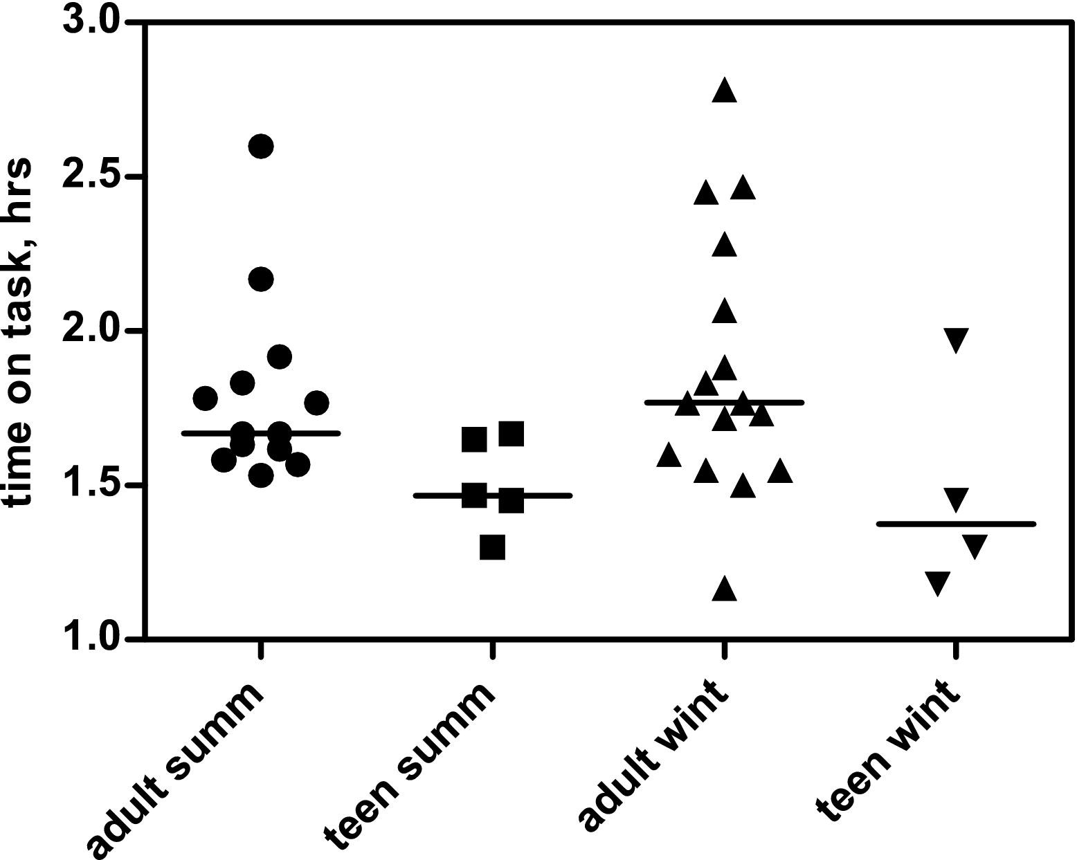
Effect of teen status on time taken to complete the course. Horizontal lines show the median value for each group of data points. Summ, summer; wint, winter.
It seems anti-intuitive that the presence of the teens strengthened an apparent relationship between speed and ESW but that the teens did not finish the course significantly faster. The most likely explanation is that the Ns being compared were too small in the latter comparison to detect significance; however, another possibility is that we are seeing a more complex interaction between the factors of adolescence and time on the course that does not parse easily with the fairly simple statistical exclusion described here. See the Discussion for more about this issue.
Discussion
In this report, we have determined summer and winter ESW values for a high- and low-visibility adult-human-size search object in a disturbed second- and third-growth, mostly deciduous, forest fairly typical of the Allegheny Plateau in southwest Pennsylvania. By conducting experiments in two seasons on the same course, we have provided the first apples-to-apples comparison of seasonal effects on visual ESW. We have also provided some insight as to the effects of different types of vegetation, albeit only in the winter, and detected a consistent, if modest, deficit in ESWs in our adolescent volunteers.
Many of our results were not surprising; in general, they confirmed the results of earlier studies,5,6 which involved larger data sets but not formal statistical analysis. The differences between high- and low-visibility search objects, leafed and denuded seasons, and vegetation thickness were predictable, but the magnitude of their effects was not. One interesting question is whether the comparatively small, if statistically significant, effect of vegetation thickness on ESW for the high-visibility search object is operationally significant.
Our study by its nature carries several significant limitations. For one thing, any investigation of this size is vulnerable to the effects of small N on statistical power. While the false-discovery correction helps guard against spurious positive results, it inevitably produces conservative conclusions that will tend to miss subtle effects. In particular, those results that produced seemingly significant P values that proved insignificant after correction (eg, the relationship between ESW and speed of searching and that between teen status and speed of searching) would seem worth future examination. Another weakness was that some of the individual measures tested (SAR experience immediately comes to mind) were self-reported, and so suffer from all the problems inherent in self-reported data.
One surprising result was the correlation of individual searchers' ESW values between different targets and different vegetation thickness. Earlier results, using percentages of targets detected, found no such correlation. 5 While it is certainly possible for ESW results to provide different results than relatively crude comparisons of detection percentages, our suspicion is that there may be a significant difference between our study and the earlier ones. We note that the great majority, if not all earlier published ground SAR ESW experiments, were undertaken as an adjunct to SAR conferences, while ours was solely an ESW experiment, though we have yet to envision a mechanism by which this difference could affect these correlations.
The phenomenon of the teen searchers' lower ESW values deserves special attention. The psychological literature suggests that teens may have cognitive difficulties in attentional tasks compared with adults 13 ; on the other hand, some researchers have found that orienteering training can help improve their visual attention capabilities. 14 For this reason, intensive training such as that offered to CAP cadets and SAR explorer scouts may help equalize search efficacy in this population with that of adults, despite the fact that SAR experience apparently is not effective in increasing ESW in other settings (however, see the argument about self-reported experience above). Since the great majority (all but one, in the summer experiment) of our teen searchers had no formal orienteering or SAR training, our study was not able to resolve this issue.
At a more fundamental level, we must bear in mind that our attempts to correlate environmental or individual factors with ESW values can demonstrate only that—correlation, not causality. While some of the correlations (such as the seasonal and object-type effects) are so strong that causality seems likely, others may not be so easily teased out with our study size and statistical methodology. More data may be necessary to feed a more sophisticated analysis that can separate the various contributions of different factors such as teen status versus speed of searching. Finally, methodological issues such as the effect of conducting the experiment along trails, if any, should be addressed in future studies, as should a more detailed examination of ESW values for clues, which our data were not able to address.
In order to most quickly reach the ultimate goal of finding the search subject, a search manager must apply search effort in a manner calculated to maximize OPOS = ∑POS = ∑(POD × POA). 7 This task requires an evaluation, at the end of each 6 hour operational period, of the cumulative PODs achieved in assigned search segments. This enables search managers to recalculate POA for each segment, and to therefore reprioritize the segments for effort in the next operational period. Since factors affecting POD calculation from ESW (including size of search team and length of path walked in the area) will differ between particular tasks of particular lost-person incidents, 6 this issue should probably enter into search managers' assessments of the effects of local terrain, vegetation, and other factors. Thus we expect that reports from searchers in the field will continue to play a role, though not a directly quantitative role, in calculating PODs for given search tasks.
Our data do imply a few recommendations for search managers. To begin with, it is useful to confirm intuitive beliefs about the effects of season, vegetation, and search-subject attire. Specifically, situations in which subjects are known or highly likely to be wearing high-visibility colors (eg, in Pennsylvania, legal deer hunters will be dressed in a minimum of 250 square inches of blaze-orange 15 ) should allow more area to be searched at a given level of coverage than situations in which the subject is in low-visibility colors (eg, a stationary turkey hunter may be wearing camouflage 15 ), given equal search effort (in the formal sense of that term; see below).
Along these lines, we would recommend a somewhat novel search method. While it is common for small “hasty” teams of trained searchers to be employed along linear travel routes early in a search, subsequent searches of segment interiors tend to involve “grid” teams, employing larger numbers of searchers spread out in more-or-less linear formation (tactics described by Syrotuck, 16 among others, but originating far earlier).
The formula for calculating POD from an ESW value is5,6:
1. POD = 1 – e−C
where C, or coverage, is:
2. C = As/Aa
As is the area effectively swept, and Aa is the size of the area being searched. As is found by:
3. As = d × n × W
where d = distance walked within search area by a single searcher, n = number of searchers (d × n defining “effort”), and W = the ESW value for that sensor (eg, type of searcher), that search object (eg, an unresponsive person wearing that color clothing), and that environment (vegetation, terrain, season, etc).
Note that ESW values are additive, both among and between tasks in a given area,5,6 and therefore the operational ESW value for a search team is:
4. Wteam = ∑Windividual
Dividing by n, we find, for the operational ESW value for a particular searcher type, environment, and search object (W, in equation 3):
5. W = Wteam/n = ∑Windividual/n ≡ Wmean
Therefore, while the non-normal characteristics of our data dictated median-based statistics to carry out the different comparisons, the ESW values we must use to operationally determine POD should be the mean values. Table 2 therefore contains operational (mean) ESW values for our local environment, broken out by significant factors in our study; note that the values in parentheses are estimated, assuming that the effect of thicker vegetation would be similar in summer and winter, when we observed it. We plan to address the issue of summer foliage effects explicitly in future experiments.
Operational (mean) effective-sweep-width (ESW) values for the Allegheny Plateau
Figures in parentheses estimated based on vegetation effects in winter.
Applying formulae 1 through 3 to our ESW data, and assuming a summer search in a 30-hectare segment for a subject wearing low-visibility colors (W = 15 m) and a desired coverage of 2 (corresponding to a POD of approximately 86%), we find that a grid team of n = 12 searchers would need to walk a path length d = 3.3 km apiece within the segment to achieve that target. Assuming a walking speed of 2 km/h, and not counting time taken to reach and return from the search segment, stop for rest breaks, etc, this would oblige them to search for 1.7 hours. This task essentially would be beyond the capabilities of a 2 person hasty team, the members of which would need to walk d = 20 km each—taking 10 hours, again assuming the same speed—to obtain a coverage of 2. As this is longer than an operational period, normally such an assignment would not even be tasked.
By comparison, the same 2 person team, searching for a high-visibility subject in the winter (W = 75 m) in the same search segment, would need to walk d = 4 km each, taking 2 hours to reach a coverage of 2. Grid teams as a rule move more slowly than hasty teams, as they are more complex to command and control, but even if we ignore this significant factor, it seems likely that the 2 person hasty team under favorable conditions of target and season is at least as effective as a 12-person grid team under unfavorable conditions, assuming the other factors are identical.
Therefore, searches for high-visibility subjects, and searches in winter conditions, might be brought to a successful conclusion via the use of far-less-manpower-expensive modes of search than are employed currently; conversely, unfavorable conditions will require more intensive modalities, such as high-n grid teams or distinct resources with potentially higher ESWs, such as air-scent search dogs. While we suspect that the current practice of using a variety of search resources will prove well-founded upon further research, we do intend to derive ESW values for other search modalities, allowing search managers to decide objectively which resources to task to which segments. We have started collecting such data. We note that this information can prove useful for optimal tasking in a nonquantitative way, for “reflex tasks” assigned in the first minutes of a search, when little on-the-ground information is available and initial, urgent efforts take priority over the detailed investigation, mapping, and planning necessary for later in the incident. 3
Regarding the lower ESW values we saw with adolescent searchers, we would argue that this finding does not in any way suggest that these searchers, when properly trained for SAR, should be excluded from operations. We should avoid the “more is better” oversimplification regarding ESW values: quantifying ESWs specifically allows us to make productive use of resources with a range of values. It may be obvious, but a lower-ESW resource that is on hand is infinitely more valuable than a higher-ESW resource that is not available—and ESW is by no means the only measure of value of a SAR resource in any case. We would think it prudent, however, not to assign adolescent searchers the longest tasks, and to make a special effort to assure that they are fully rested and rehydrated before retasking them after they return from the field.
In this report we have derived ESW values for searchers in the typical environments for rural and wilderness searches in southwest Pennsylvania. By adding statistical analysis to the methodology established in previous reports, we have provided a tool to determine whether observed differences in ESW value are likely to be real, or only an artifact of random variability. In future reports we will tackle some of the limitations posed by the present study and expand to cover other operationally important factors.
Footnotes
Funding
The authors would like to thank the members of Allegheny Mountain Rescue Group who helped set up and tear down our 2 experiments and who commented on this manuscript; T. Madison of Alpha Team K-9 SAR and Rabun County EMA Rescue Team, Georgia, who also helped with setup; AMRG's leadership and members, for financial support from the team's general budget in obtaining some of the equipment used; as well as members of AMRG, Civil Air Patrol Squadron 1407, Fayette County Search and Rescue, the Youth Outdoors program of Cleveland Metroparks and 4H, and the individual volunteers who came out to participate as searchers and loggers in our ESW experiments. Thanks also go to GraphPad company for donating its Prism software package to AMRG. Particular thanks go to R.J. Koester, for continuing advice and guidance on ESW experimentation and protocols, and to the Commonwealth of Pennsylvania Game Commission, for permission to conduct the experiment and for special access to the Game Lands.