Electrothermal Fluid Manipulation of High-Conductivity Samples for Laboratory Automation Applications

Abstract

Electrothermal flow is a promising technique in microfluidic manipulation toward laboratory automation applications, such as clinical diagnostics and high-throughput drug screening. Despite the potential of electrothermal flow in biomedical applications, relatively little is known about electrothermal manipulation of highly conductive samples, such as physiological fluids and buffer solutions. In this study, the characteristics and challenges of electrothermal manipulation of fluid samples with different conductivities were investigated systematically. Electrothermal flow was shown to create fluid motion for samples with a wide range of conductivity when the driving frequency was greater than 100 kHz. For samples with low conductivities (below I S/m), the characteristics of the electrothermal fluid motions were in quantitative agreement with the theory. For samples with high conductivities (greater than l S/m), the fluid motion appeared to deviate from the model as a result of potential electrochemical reactions and other electrothermal effects. These effects should be taken into consideration for electrothermal manipulation of biological samples with high conductivities. This study will provide insights in designing microfluidic devices for electrokinetic manipulation of biological samples toward laboratory automation applications in the future.

Introduction

The development of automated microfluidic systems poses great promises for a variety of medical diagnostic applications.^1–3 Although extensive research efforts have been devoted to integrate various transduction mechanisms, including optical, inertial, interfacial, and electrochemical sensing, the transducers often require sample preparation components for handling clinical samples.^4–7 The implementation of the sample preparation modules, which critically determines the overall performance of the system, can often be cumbersome, labor intensive, and time consuming, and represents a major challenge for laboratory automation.^8,9 Among numerous microfluidic techniques, alternating current (AC) electrokinetics is one of the most promising approaches for addressing this fundamental hurdle in laboratory automation.^10–12 AC electrokinetics is especially effective in the micro and nano domains and can be easily integrated with other microfluidic components. Furthermore, combinations of different electrokinetic phenomena allow fundamental fluidic operations, including concentration, separation, mixing, and pumping, to be performed in the same platform.^13–15 Electrokinetics has also been applied in various mechanobiological applications.^16,17 All these features render electrokinetics one of the most promising approaches for developing fully integrated microfluidic diagnostic systems for laboratory automation.^18,19

Most electrokinetic techniques, such as dielectrophoresis and AC electroosmosis, are effective only in low-conductivity fluids. Electrothermal flow, on the other hand, is effective in fluids that have a wide range of conductivity. The effectiveness of electrothermal flow in samples with high conductivities, such as biological buffers and physiological fluids (on the order of 1 S/m), contributes to its general applicability in laboratory automation applications. Electrothermal flow is typically observed at frequencies greater than 100 kHz. ²⁰ When an external electric field is applied across the electrode, Joule heating creates temperature gradients near the electrode. The temperature gradient induces permittivity and conductivity gradients. The interaction between the electric field and the gradients, as a result, creates a bulk electrical force causing fluid motion.

A theoretical model has been developed previously to reveal the characteristics of electrothermal flow.^21,22 Neglecting convection that is slow compared with thermal diffusion in typical operating conditions, the temperature distribution at equilibrium can be estimated by balancing Joule heating and thermal diffusion.

$$k{\nabla }^{2}T+\sigma E^2=0$$

(1)

where k is the thermal diffusivity, T is the temperature of the medium, σ is the conductivity of the medium, and E is the applied electric field. Rearranging Eq. (1) provides an order of magnitude estimation of the temperature rise,

$$\Delta T\approx \sigma V^2/k$$

(2)

Equation (2) describes the general dependence of the temperature rise, and more accurate temperature estimation has also been performed.^21,22 As conductivity and permittivity gradients are induced because of the temperature gradient, an electrical force on the bulk fluid is created as a result of the interaction between the electric field and the gradients. The time-averaged electrothermal force, 〈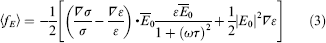f_E〉, has been estimated to be

$$〈f_E〉=-\frac{1}{2}\left[\left(\frac{\nabla \sigma }{\sigma }-\frac{\nabla \epsilon }{\epsilon }\right)·{\overline{E}}_0\frac{\epsilon {\overline{E}}_0}{1+{\left(\omega \tau \right)}^2}+\frac{1}{2}{\left|E_0\right|}^2\nabla \epsilon \right]$$

(3)

where ω is the angular frequency of the applied potential, ∊ is the permittivity, and E₀ is the magnitude of the electric field. The first and second terms on the right hand side of Eq. (3) represent the Coulomb force and the dielectric force, respectively. The charge relaxation time, τ, is the ratio between the permittivity and the conductivity, τ = ∊/ω. An analytical expression of the time-averaged electrothermal force has been derived for a parallel electrode with a small gap.

$$〈f_E〉=-M\left(\omega ,\hspace{0.17em}T\right)\left(\frac{\epsilon \sigma V_{\text{rms}}^4}{2k{\pi }^3{r}^{3}T}\right)\left(1-\frac{2\theta }{\pi }\right){\stackrel{⌢}{n}}_{\theta }$$

(4)

$$M\left(\omega ,\hspace{0.17em}T\right)=\left(\frac{T/\sigma \hspace{0.17em}\partial \sigma /\partial T-T/\epsilon \hspace{0.17em}\partial \epsilon /\partial T}{1+{\omega }^2{\tau }^2}+\frac{1}{2}\frac{T}{\epsilon }\frac{\partial \epsilon }{\partial T}\right)$$

(5)

where r and θ are the radial and angular coordinates, respectively. M(ω, T) represents the frequency dependence of the electrothermal force. The induced electrothermal profile can be estimated by considering the Navier-Stokes equations.

$$\eta {\nabla }^2\overline{v}-\nabla p+\overline{f}=0$$

(6)

$$\nabla ·v=0$$

(7)

where η is the viscosity, ν is the velocity, p is the pressure, and f is the bulk fluid force. The electrothermal velocity can be approximated as $\overline{v}\approx \left|\overline{f}\right|\frac{l^2}{\eta }$ using the first-order approximation and is roughly proportional to the bulk fluid force.

This theoretical analysis reveals several key characteristics and practical considerations of electrothermal fluid manipulation. First, the temperature rise approximation indicates that the temperature of the sample can be greater than 100 °C in some conditions. This is especially important when the conductivity of the sample is high. A high temperature could lead to degradation of the samples (e.g., proteins) and other unwanted electrothermal effects. Second, electrothermal flow depends on the applied frequency. The Coulomb force dominates at low frequency, whereas the dielectric force dominates at a high frequency. The crossover of the dominance and change in the flow direction occur at a frequency of the order of the inverse of the charge relaxation time. Third, the electrothermal force and the fluid velocity have strong voltage dependences (to the fourth power) on the applied voltage. Within the context of laboratory automation, it is the most effective operating parameter for regulating the electrothermal force for sample preparation applications.

Recent studies of electrothermal flow have demonstrated that a biotin-streptavidin binding assay can be enhanced by electrothermal stirring.^23,24 Micropumps based on electrothermal flow have also been proposed by using an array of asymmetric pairs of electrodes.^25,26 On the other hand, a combination of electrothermal flow and other electrokinetic effects has been demonstrated for particle trapping, concentration, separation, mixing, and pumping.^27–30 In addition to Joule heating—induced electrothermal flow, optoelectrical fluid motion has been reported for particle manipulation.^31–33 Nevertheless, relatively little is known about the fundamental characteristics and practical limits for electrothermal manipulation of fluids with high conductivities. In this article, we perform a systematic investigation on electrothermal manipulation of fluids with a wide range of conductivities. The results could potentially serve as guidelines in the design of electrothermal flow—based microfluidic devices for laboratory automation applications.

Materials and Methods

A concentric electrode design was applied to generate three-dimensional vortices in a microfluidic chamber. The outer diameter and gap distance of the concentric electrodes are 550 and 50 μm (Fig. 1A). The electrodes were deposited by evaporating 300-nm gold on a glass substrate with a 50-nm chromium adhesion layer and were patterned by lift-off. The microfluidic chamber was created by placing a cover slip and spacers of 170 (μm on top of the substrate. The AC driving voltage was generated by a function generator (33120A; HP, Everett, WA.). The inner and outer electrodes were connected to the driving signal and the ground, respectively. The potential drop across the microelectrode was monitored by a digital storage oscilloscope (GDS-1102; GW Instek, Taipei, Taiwan) and reported as the voltage values.

Figure I.

(A) Schematic of the concentric electrode for characterizing electrothermal flow. (B) Visualization of the particle trajectories by overexposure to the CCD camera for 13 s.

The experiments were performed using buffer of 1 × tris-ethylenediaminetetraacetic acid (EDTA) with conductivities from 0.01 to 22 S/m. The conductivity of the solution was adjusted by addition of sodium chloride. The solutions were seeded with 200-nm florescent particles (F8810; Invitrogen, Carlsbad, CA) for flow visualization. All velocity measurements were performed 100 (μm above the gap of the concentric electrode to avoid the dielectrophoretic effect on the tracer particles. ³⁴ The microfluidic chamber was loaded onto an epi-fluorescence microscope (DMI 4000B; Leica, Frankfurt, Germany). The particle motion was captured with a digital charge-coupled device (CCD) camera (DMK31AF03; Image Source, Bremen, Germany) at 30 frames per second. All experiments were performed at room temperature (22 °C).

Fluorescence images were analyzed with Matlab (The MathWorks, Natick, MA) and ImageJ (National Institutes of Health, Bethesda, MD). At least eight particles were traced for each velocity measurement, and the results were reported as the mean ± standard error of the mean. The exponent, ℓ, of the voltage dependence of the electrothermal velocity, v, was fitted using the power-law relationship, v = CV^e, where V is the root-mean-square voltage (V_rms) and C is an empirical constant depending on the geometry of the electrode and other operating conditions. The results were reported as the mean ± standard error of the fit.

Results

In the experiment, three-dimensional fluid motions were observed on the concentric electrode. The flow patterns were similar for different operating conditions. Figure 1 B show a representative image of the flow pattern by tracing the particle trajectory. The conductivity was 1 S/m, and the applied voltage and frequency were 6 V peak to peak and 200 kHz, respectively. It should be noted that the fluid motion extended to regions as far as 300 (μm outside the electrode, which is approximately the same as the radius of the outer electrode.

The fluid velocity was measured at different frequencies (100—13 MHz) to investigate the frequency dependence of the observed fluid motion. Lower voltages were applied to samples with higher conductivities to avoid electrolysis and bubble formation. Figure 2 shows the frequency dependence of the fluid motion. For 0.01 S/m, the velocity at low frequency was approximately constant. The flow motion changed to the opposite direction at high frequency, and the frequency of the transition occurred approximately at 5 MHz. For 0.1 S/m, a decreasing trend of the fluid velocity was observed at high frequency (from 10 to 15 MHz). Higher frequency was not characterized because of the limitation of the operating frequency range of the function generator. For higher conductivities (1.3 and 22 S/m), the electrothermal velocities remained constant in the frequency range tested.

Figure 2.

Frequency dependence of the fluid velocity. Applied voltages are sinusoidal waveforms with peak-to-peak voltages of 20, 16, 10, and 8 V for conductivities of 0.01, 0.1, 1.3, and 22 Sm⁻¹, respectively. Error bars represent the standard error of the mean.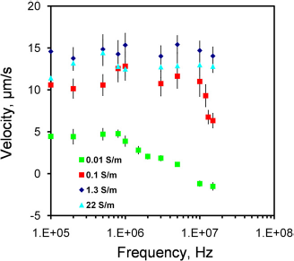

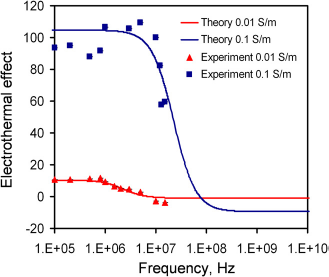
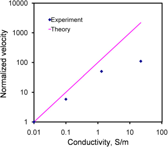
The frequency dependence of electrothermal flow estimated by the model is shown in Figure 3. The model suggested that the electrothermal force and crossover frequency increased with the conductivity of the medium. Because the electrothermal force is linearly proportional to the velocity, we normalized the force estimated by the model and the velocity measured from the experiment to compare the frequency dependence of the fluid motion (Fig. 4). For 0.01 and 0.1 S/m, excellent agreement was obtained between the experiment and the model. For 0.01 S/m, the predicted crossover frequency was 4.46 MHz, and the value observed was 5 MHz. For 1 and 22 S/m, the crossover frequencies were predicted to be 0.446 and 9.8 GHz, which were outside the frequency range tested. As expected, the electrothermal effects remained constant in both the experiment and the model for the frequency rangebeing examined. Furthermore, wenormal-ized the force estimated by the model and the experimentally measured fluid velocity with the fourth power of the applied voltage (see Eq. (3)) at 200 kHz to study the conductivity dependence (Fig. 5). For low conductivities (0.01-1 S/m), the normalized velocity scaled linearly with the conductivity, as suggested by the model. Both the frequency and conductivity dependence studies indicated that the observed fluid motion was a result of electrothermal flow. For high conductivity (22 S/m), although the fluid motion displayed similar frequency dependences, the amplitude of the velocity deviated significantly from the value predicted.

Figure 3.

The frequency dependence of the electrothermal force for different conductivities calculated by the model. Voltages are sinusoidal waveforms with peak-to-peak voltages of 20, 16, 10, and 8 V for conductivities of 0.01, 0.1, 1.3, and 22Sm⁻¹, respectively.

Figure 4.

Comparison of the frequency dependence of the experimental results with the model for samples with conductivities of 0.01 and 0.1 Sm⁻¹.

Figure 5.

Comparison of the conductivity dependence of the experimental results with the theoretical calculation. The velocities were normalized with the fourth power of the applied root-mean-square voltage to compare the conductivity dependence. Error bars represent the standard error of the mean.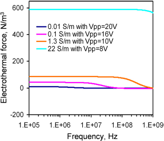

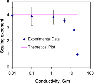
To better understand the effect of the conductivity, the voltage dependence of the fluid velocity was characterized. The applied frequency was 500 kHz. Figure 6 shows the voltage dependence of the fluid velocity from 0.01 to 22 S/m. Generally, the velocity increased with the applied voltage and the conductivity. The velocity-voltage relationship displaced the power-law dependence. According to the model, the electrothermal force should have a fourth-power dependence on the electric field. Figure 7 summarizes and compares the scaling exponents predicted in the model and observed in the experiment. For conductivities between 0.01 and 1 S/m, the velocity approximately scaled to the fourth power of the applied voltage. It should be noted that AC electroosmosis and dielectrophoresis have second-power dependence on the applied voltage. It was further verified by the results that the observed fluid motion was a result of electrothermal flow, and the model was able to capture the frequency dependence of the observed fluid motion at low conductivity. However, the exponents deviated from the model and decreased from 3.8 to less than 1 when the conductivity increased from 1 to 22 S/m. This was likely to be the result of other phenomena that are sensitive to the conductivity of the sample.

Figure 6.

Voltage dependence of the fluid velocity at 200 kHz. Data represent mean ± standard error of the mean.

Figure 7.

Comparison of the power exponent for the electrothermal force and the applied electric field of the experimental data with the theory at different conductivities. Error bars represent the standard error of the fit.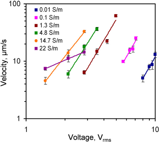

Discussion

Our results suggest that electrothermal flow is a dominant electrohydrodynamic effect when the applied frequency is greater than 100 kHz. The observed fluid motion cannot be explained by other electrohydrodynamic effects, which have different frequency and voltage dependences. For instance, AC electroosmosis is only effective at low frequency (less than 100 kHz) and has a second-power dependence on the applied voltage. ¹⁰ On the other hand, Joule heating-induced temperature gradient can create a difference in fluid density and results in buoyancy force.^21,22 The buoyancy force, f_B, is given by

$$f_B=\frac{\partial {\rho }_m}{\partial T}\Delta Tg\sqrt{a^2+b^2}$$

(8)

where ρ_m is the fluid density, g is the standard gravity, and &Delta T is the temperature rise, which can be estimated from Eq. (2). Numerical calculation reveals that the ratio between the buoyancy force and the Coulomb force is less than 0.1 in our experimental condition. This suggests that the buoyancy force is unlikely to be a dominant effect in our experiment conditions.

Our experimental data suggest that the electrothermal flow is applicable to samples with a wide range of conductivities. As shown in Figure 5, similar electrothermal velocity can be obtained in samples with conductivities spanning across three orders of magnitude by adjusting the applied voltage. A lower voltage is needed for manipulating a sample with a higher conductivity. This presents a unique advantage of electrothermal flow for biomedical applications. The technique is highly effective with physiological fluids, including blood urine and saliva, which have conductivities of the order of 1 S/m.

In the experiment, we observed discrepancy between the experimental data and the model. The aberrancy could be a result of the idealistic assumptions in the model. With a highly conductive buffer, electrochemical reaction at the electrode surfaces, which is not considered in the model, may no longer be neglected. In fact, we observed degradation of the electrode surfaces (Fig. 8). These electrochemical reactions may reduce the effective potential across the electrode and the resulting electrothermal effect. Second, the temperature rise is assumed to be small in the derivation of the electrothermal force. Nevertheless, the estimated temperature rise can reach greater than 100 °C based on the order of magnitude estimation. This presents uncertainties in the linear approximation and the boundary conditions applied in the model. As a result, the assumption that the buoyancy effect is negligible may no longer be valid. Furthermore, evaporation, which could further increase the effective conductivity of the sample, became significant in our experiment. We noticed that, by applying AC potential with a peak-to-peak voltage of 6 V and frequency of 200 kHz, the conductivity of the buffer increased from 10 to 13 S/m in 5 min. Further theoretical and experimental investigation, for example, measuring the temperature distribution of fluids with different conductivities, will be necessary to elucidate the roles of these electrothermal, buoyancy, and electrochemical effects on electrothermal fluid manipulation.

Figure 8.

The electrode surface (A) before and (B) after the application of a voltage of 8 V peak to peak and frequency of 200 kHz for 1 min. The conductivity of the sample was 5 S/m.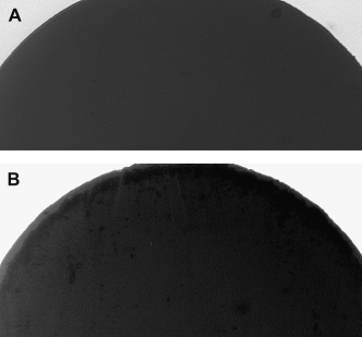

Conclusions

Electrothermal flow is one of the most effective AC electrokinetic techniques for laboratory automation because of its effectiveness at physiological conductivity (∼1 S/m). Despite the discrepancy in the model, our results demonstrated that electrothermal flow is highly effective for the manipulation of fluids with a wide range of conductivities. Our result will serve as a guideline for performing effective sample preparation procedures using the electrothermal processing. In situ characterization of the sample conductivity using impedance spectroscopy or other techniques could be integrated into the microfluidic system for handling samples with unknown conductivities.