
Abstract
An automated instrument was designed and constructed to facilitate the performance of pharmaceutical degradation studies. A brief theoretical background on degradation kinetics is given to rationalize the design of the instrument and representative data are provided to illustrate its successful application. This system was found to be capable of conducting multiple simultaneous isothermal and nonisothermal kinetic studies with user-defined temperature profiles, sampling periods, and data logging.
Keywords
INTRODUCTION
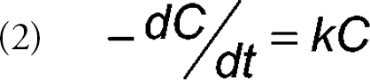
The development of a pharmaceutical drug candidate is greatly assisted by the acquisition of information on the rates and pathways of degradation of the active pharmaceutical ingredient and formulation(s). Rate and product distribution data can be used, for example, to choose appropriate salt forms or polymorphs, to optimize formulations for maximum stability, to predict shelf lives of drug products and outcomes of real-time stability studies, and to determine the major degradation pathways. Typically, such studies are conducted under multiple sets of conditions (e.g., temperature, pH, etc.). Often the Arrhenius equation (Equation 1) is used to correlate reaction rates (k) with temperature:
where A is the frequency of molecular collisions, E is the activation energy, R is the gas constant, and T is the absolute temperature. This equation can be applied to both isothermal and non-isothermal studies. These kinetics and product distribution studies involve the sampling of the reaction mixture over time and subsequent analysis of these samples. Manual sampling can be tedious and simply missing a sampling point makes the data less valuable. Presented here is a description of the design and construction of an instrument that automates these kinetics and product distribution studies. The automated instrument is capable of managing temperature and sampling of up to three simultaneous isothermal and/or nonisothermal reactions (i.e., 40 vials/reaction).
BACKGROUND
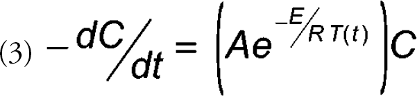
Traditionally, degradation reactions of pharmaceutical compounds have been studied under isothermal conditions and rate constants have been measured at multiple temperatures. As an example, the data for a first-order reaction can be modeled with a differential rate equation in which the decrease in the concentration of parent drug (-dC/dt) is directly proportional to the concentration of the drug at time t (equation 2) where k is the rate constant and C is the concentration of the parent drug at time t. Prediction of reaction rates at temperatures that are not studied can then be derived from the Arrhenius equation (equation 1). Typically, experimental data are acquired at three or more temperatures.
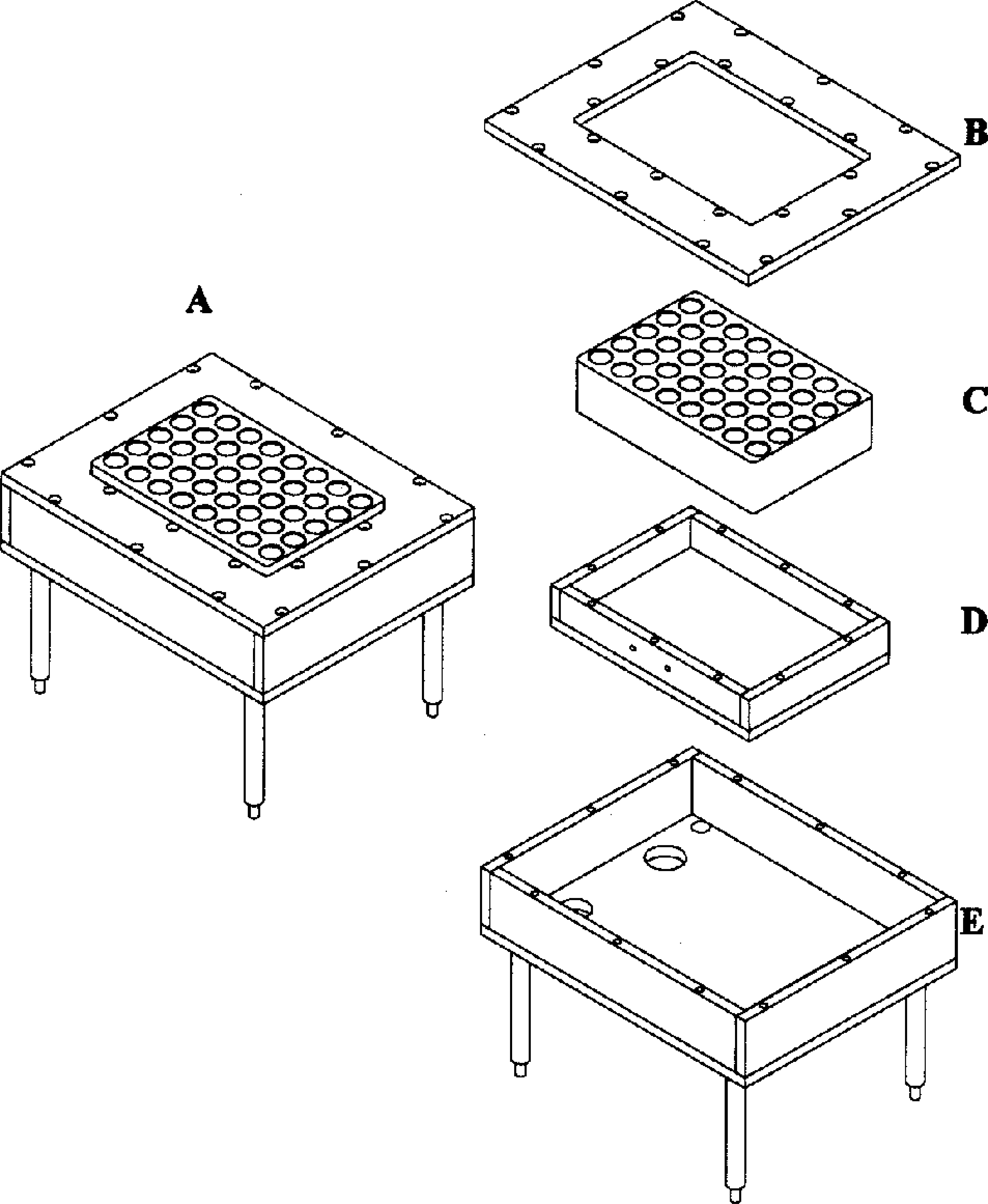
Alternatively, equivalent rate data (i.e., the ability to calculate rate constants at any temperature) can be obtained in one experiment using the nonisothermal approach in which a temperature program is used. 1,2 The resulting data are fitted with a rate equation that contains terms for temperature and the concentration of the drug. Thus, for a first-order reaction, equations 1 and 2 can be combined to give equation 3 where the temperature, T(t), is a function of time. The utilization of various temperature functions have been reported and are summarized in Table I. Once the activation energy (E) and the frequency factor (A) have been determined by fitting the data to a model such as equation 3, rate constants are then calculated for various temperatures by the use of equation 1. Comparison studies of this nonisothermal approach with isothermal approaches have given nearly identical results. 1 –7 Thus, the use of nonisothermal techniques for accelerated drug degradation studies seems appropriate as a means to acquire more data concerning the behavior of the drug candidate in a limited time.
Nonisothermal models used for degradation kinetics data.
RATIONALE FOR INSTRUMENT DESIGN
In general, conducting isothermal or nonisothermal degradation reaction studies involves:
obtaining sufficient data points (usually 30–40) to obtain a good fit for the kinetics models,
conducting multiple reactions in parallel to complete the study within a reasonable time period,
programming the desired temperature profiles,
programming sampling intervals,
maintaining solutions of the drug formulation or samples of the drug substance at programmed temperatures,
removing samples of the reaction product mixtures at programmed intervals,
storing the samples at a low enough temperature to quench the reaction,
recording of actual reaction temperatures,
recording of actual sampling times,
analyzing the samples by techniques such as high performance liquid chromatography (HPLC).
Analyses of samples using HPLC (operation 10) can be performed in an automated fashion using commercially available instrumentation. Therefore, the automated instrument was designed and constructed to perform operations 1–9 exclusively. Although HPLC analysis (operation 10) was not incorporated into the automated instrument, provisions were made for the optional use of HPLC autosampler vials as reaction vessels. Thus, the instrument consisted of three “hot blocks” for heating up to 40 reaction vessels in each block (2-mL vials), three “cold blocks” for storage of these reaction vessels prior to analysis, an “autosampler” for moving sample vessels from the hot block to the cold block, a temperature controller to regulate the temperatures of the hot and cold blocks, and a computer program for a user interface and data logging. If HPLC autosampler vials are used, then the user has the option of simply transferring the autosampler vials from the cold block to an HPLC system for analysis.
An alternative design might have involved a single reaction vessel rather than multiple independent reaction vessels. The independent reaction vessel approach was taken for several reasons. First, a single reaction vessel would not be feasible for solid state reactions since sample aliquots could not readily be set aside. In addition, we often prefer to pre-weigh solid-state reaction samples that are to be conducted in open vessels in case there is a loss or gain of water during the reaction period. Second, with liquid reactions, contamination might occur during sampling from a single reaction vessel. 3,8 Third, material for each time point is often required for multiple analyses (HPLC, HPLC-MS, etc.) and therefore several samples would be required in any case. And fourth, using smaller, multiple reaction vessels allows for “sample limited” situations.
For maximum flexibility, each reaction block could be independently programmed with either a time/temperature equation such as any of the approaches given in table 1 or with a user-generated time versus temperature table. Thus, the instrument can support simultaneous isothermal studies and nonisothermal studies with any conceivable temperature program. Although the instrument shown here has only three blocks, a larger system could be designed to accommodate additional reactions. Continuous data logging provided a convenient audit trail to ensure that the actual temperatures of a defined study followed user prescribed temperatures. 9
DETAILED DESCRIPTION ON INSTRUMENT
Hot and Cold Block Design
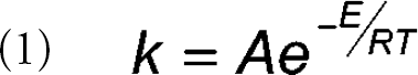
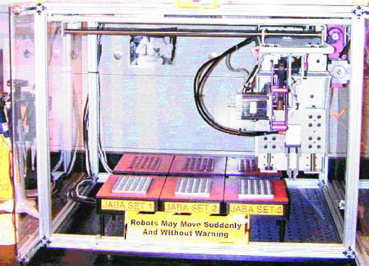
The removable hot and cold blocks were made of aluminum and contained holes to accommodate 40 reaction vessels (Figure 1). The blocks could accommodate standard HPLC autosampler vials (2-mL; Chromacol - Trumbull, Conneticut, USA, PN: 2-CV) with silicon Teflon crimp caps (Chromacol - PN: 11-AC-ST15) or glass sealed ampules (2-mL pre-scored ampules; Wheaton Science Products - Millville, NJ, USA, PN: 176776). The crimp cap vials could be used with temperatures up to 100 °C while the glass sealed vessels could be used with temperatures up to 200 °C.
Hot and cold blocks shared a common mechanical design
A silicone rubber heater (Watlow Electric Manufacturing Company - St. Louis, Missouri, USA, PN: F030050C7-A001B) with an etched foil element provided uniform heating of the reaction vials in the hot block. A thermal electric cooler (Marlow Industries - Dallas, TX, USA, PN: ST3353–02) cooled the reaction vials in the cold plate to 5 °C ± 1 °C. The hot and cold blocks were insulated with one-inch thick melamine white foam (McMaster Carr - New Brunswick, NJ, USA, PN: 86145K54). A high precision resistive temperature detector (RTD) (Watlow Electric Manufacturing Company, PN: S80–1000204) monitored the temperatures of the blocks. The temperatures of the blocks were controlled by a dual loop temperature controller (Watlow Electric Manufacturing Company, PN: 999D-22CC-AURG). The controller provided a voltage signal (24 VDC) to regulate the power to the heating (120 VAC) and cooling units (12 VDC) via solid-state relays (Grayhill - La Grange, IL, USA, PN: 70S2–04-B-06-N; 70S2–01-A-05-N respectively). Power for the thermoelectric cooler (TEC) was provided by a switching regulated (12 VDC/4.1 amp) power supply (Acopian - Easton, PA, USA, PN: 12WB410). The temperature controller held the blocks to within 0.1 °C of the user-defined temperature. The standard deviation of temperature between the reaction vials within the hot and cold blocks was 0.3 °C and this value was comparable to systems reported in the literature. 10,11
Autosampler
A three axis robotic workcell (Arrick Robotics - Hurst, TX, USA, PN: RW-18b-3-Axis) served as the autosampler (Figure 2). Stepper motors and pulley reducers on each axis provided precision movements accurate to within 0.002′. Power supplies for the stepper motors were provided with the unit. A pneumatic gripper (SMC Corporation of America - Indianapolis, Indiana, USA, PN: MHQ2–16D) was mounted on the z-axis (Figure 3). Custom designed fingers allowed the sample vials to be moved from the hot to the cold blocks. The gripper was operated by toggling a 20 p.s.i. pressure between one of two lines. One line opened and the second closed the gripper. The two lines were regulated by a solenoid valve that, upon activation, pressurized the “closed” line and vented the “open” line.
Robotic workcell for autosampling of vials over the course of the experiment.
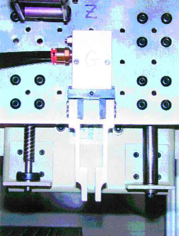
Gripper Assembly used to pick and place vials from the hot to the cold blocks.
System Integration
A standard desktop computer (IBM 233 MHz, 32 MB RAM) controlled the instrument. A custom program written in LabVIEW 5.1® (National Instruments - Austin, Texas, USA) allowed the user to specify the desired temperature and exposure time for each vial in the hot block (Figure 4). All temperature equations listed in table 1 were capable of being programmed through this interface. Alternatively, a tab delimited file with time and temperature columns could be imported. After identifying the experimental conditions on this user interface, the user loaded the vials into the preheated hot block and the experiment was subsequently started.
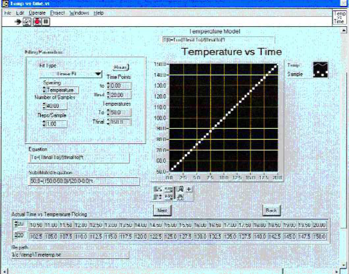
User interface for programming temperature profile for degradation experiment. Squares identify time intervals when vials will be moved from hot to cold blocks.
The master control panel for the experiment is shown in Figure 5. A master clock tracked the experimental time and the secondary clock tracked the time until the next vial was to be moved from the hot to the cold block. A pictorial simulation of the 40-position hot and cold blocks was presented to the user. The figure demonstrates an experiment that was 4.5 hours into a 20-hour study. The status of the vials was shown by respective color changes in the hot and cold block positions. A thermometer provided the current temperature for each block. The graph below the thermometer tracked the experimental temperature of the hot block over time.
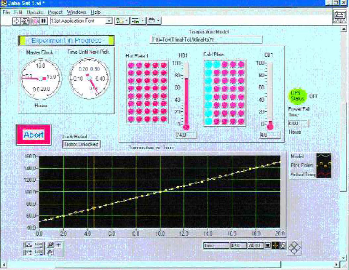
Master control panel tracking temperatures and position of vials. Master clock is the relative time for the experiment. Simulated views of the hot and cold blocks provide a pictorial view of the current location of all vials. Thermometers reflect the actual temperature of each plate. The graph tracks the actual temperature of the hot block as a function of time.
During the course of an experiment, the temperature controller was updated every 0.1 °C change in the user defined temperature profile. A tab delimited text file logged actual temperature changes greater than 0.1 °C for either the hot or cold blocks. The file also captured the sampling time of each vial. The text file provided a convenient audit trail for the user.
APPLICATION
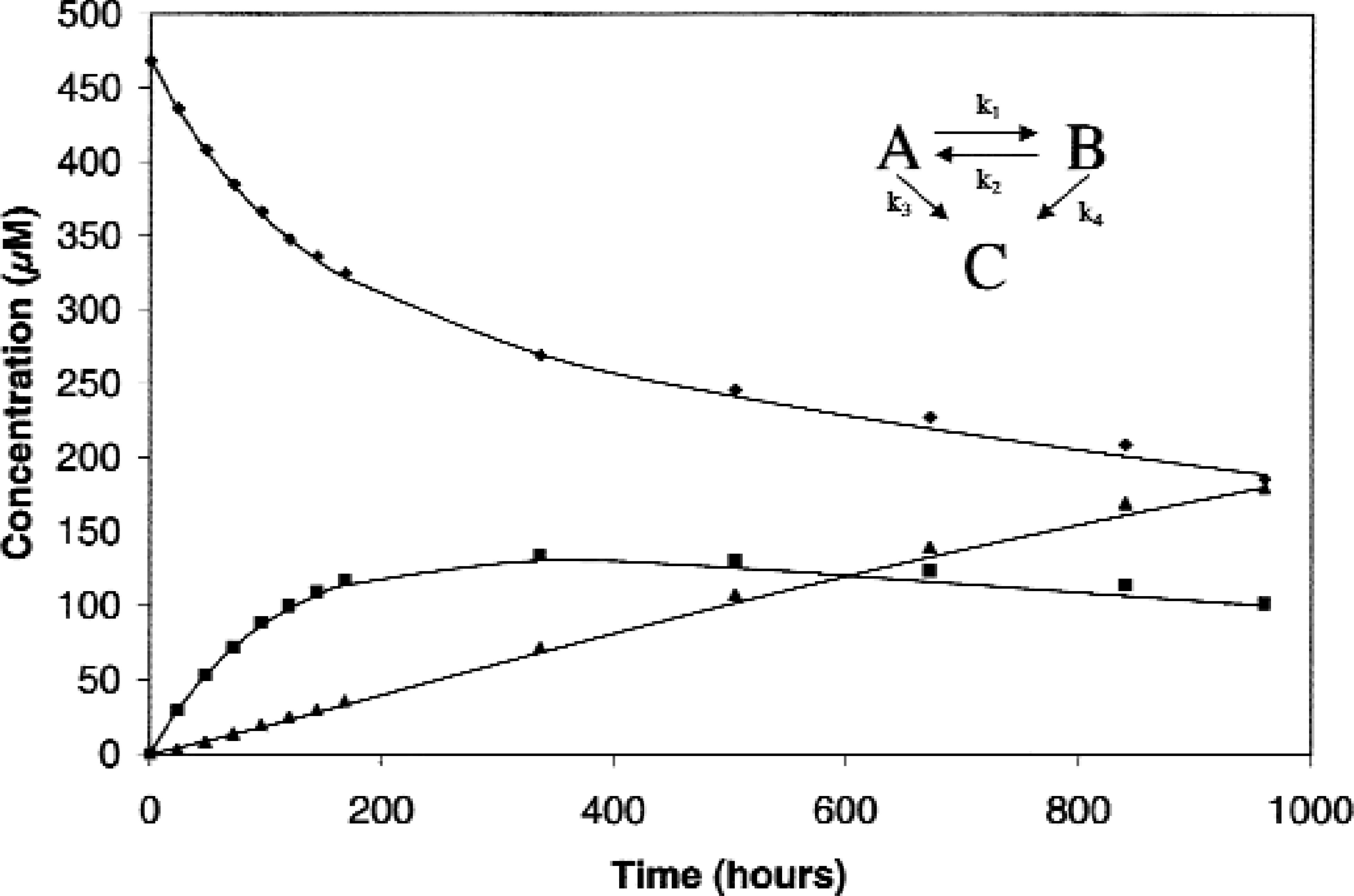
The system described above has been applied to the study of several compounds under development as new pharmaceutical agents. The system has shown itself to be of great utility in increasing the efficiency and accuracy of performing these necessary drug characterization studies. To provide one example, the system was used to elucidate the degradation chemistry of a new drug candidate whose structure suggested a susceptibility to aqueous reactivity. In solution, the drug molecule (A) could potentially undergo acyl migration to give a re-arrangement product (B) or hydrolysis of the acyl moiety to give the hydrolyzed form of the drug (C). In addition, the re-arranged form (B) can also convert to the hydrolysis product (C).
The reaction scheme and the data (i.e., drug and drug degradation products molar concentrations versus time plot), from the above example are shown in Figure 6. The temperature of the reaction block was 40 °C and the temperature of the cold block was 5 °C. HPLC analyses were conducted within 24 hours of sampling and selected traces are shown in Figure 7. Samples were assayed daily during the first week of the experiment when the loss of drug was most rapid. This allowed better fitting of the experimental data over this more curved region of the plot. To maximize efficiency of HPLC assay time and resources, samples were assayed only weekly during the more linear later region of the degradation profile.
Degradation profile of a low molecular weight compound performed on the robotic instrument described here.
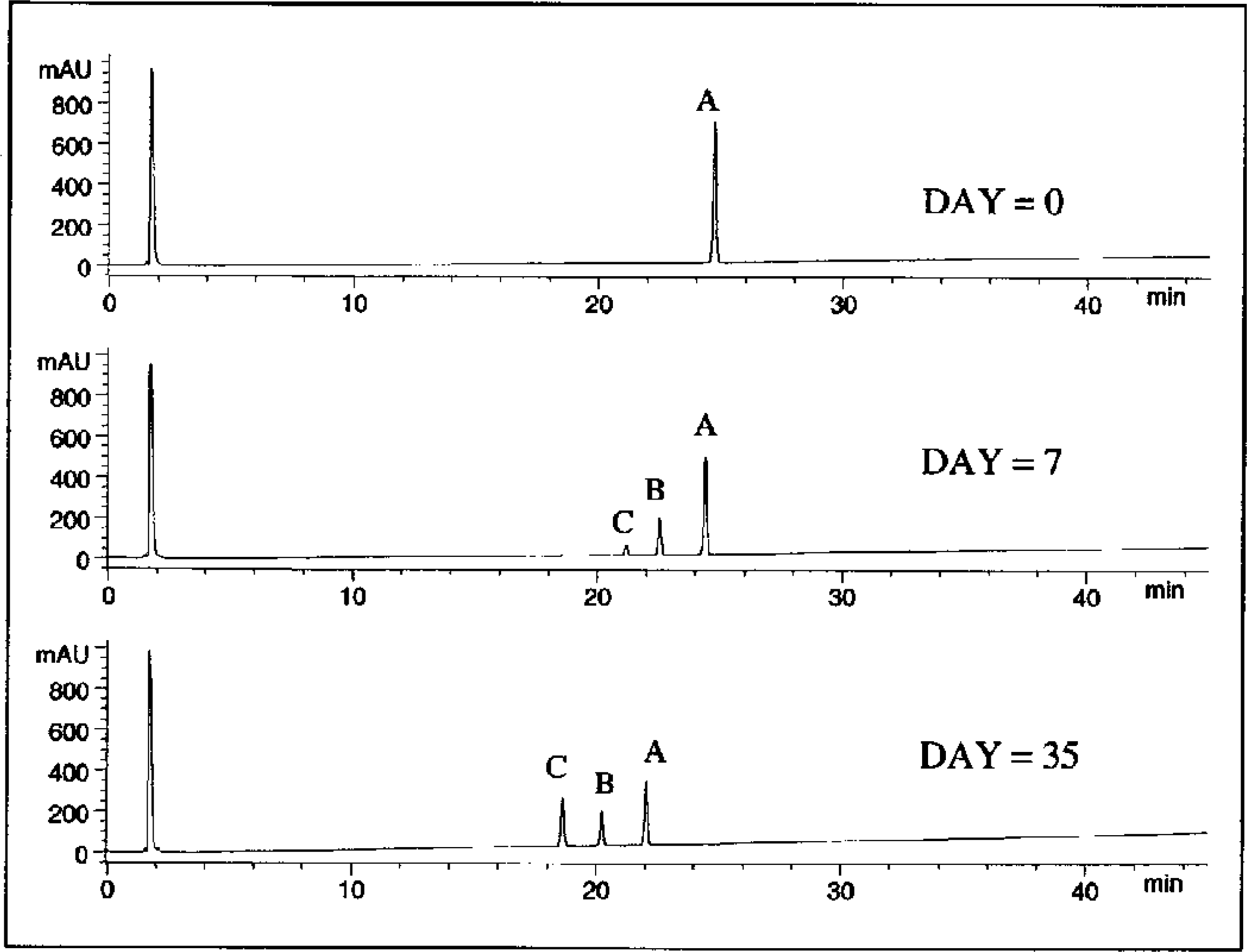
Selected chromatograms of samples that were analyzed on an Agilent 1100 HPLC system.
The experimental results clearly demonstrated the degradation profile expected for a molecule of this type. 12 The drug substance (A) most rapidly equilibrated with the re-arrangement product (B), with a slower conversion of both A and B to the terminal product C via hydrolysis. Rate constants were obtained by least squares fitting of the data to the differential rate equations for the reaction scheme (Figure 6; Scientist Version 2.0, MicroMath Scientific Software, Salt Lake City, UT). These rate constants were: k1 = 2.91 ± 0.07 × 10⁻³ h−1, k2 = 5.2 ± 0.2 × 10⁻³ h−1, k3 = 3.5 ± 0.4 × 10⁻⁴ h−1, and k 4 = 8.5 ± 1 × 10⁻⁴ h−1. The resulting fitted curves are shown in Figure 6.
SUMMARY
The automated instrument described here is capable of performing both isothermal and nonisothermal experiments. We have demonstrated the utility of the instrument to carry out routine isothermal kinetic determinations. Currently, the instrument is capable of performing three simultaneous and independent reactions with 40 vials per reaction (Figure 3). A second instrument capable of conducting 16 independent reactions is being designed. Kinetics studies are extremely labor intensive and these instruments remove all of the redundant tasks as outlined above. Therefore, such instruments are useful in rapidly screening many potential molecules for their suitability as drug development candidates based on their potential stability. The performance of such studies early in development can also play a key role in formulation design and product development. The system outlined here has been able to save time and labor for the chemists performing these reactions by enabling unattended sampling and accurate temperature profiles.