
Abstract
This article is concerned with developing an intelligent system for the control of a wheeled robot. An algorithm for training an artificial neural network for path planning is proposed. The trajectory ensures steering optimal motion from the current position of the mobile robot to a prescribed position taking its orientation into account. The proposed control system consists of two artificial neural networks. One of them serves to specify the position and the size of the obstacle, and the other forms a continuous trajectory to reach it, taking into account the information received, the coordinates, and the orientation at the point of destination. The neural network is trained on the basis of samples obtained by modeling the equations of motion of the wheeled robot which ensure its motion along trajectories in the form of Euler’s elastica.
Keywords
Introduction
At present, the optimal path planning for mobile robots is based, as a rule, on the analysis of the kinematics or dynamics of their motion. As optimality criteria, one can use various parameters, for example, maximal speed, minimal path length, minimal or maximal acceleration, the requirement to ensure the specified orientation, and their combinations. 1 –4 However, due to the specificity of applied problems, the results of theoretical analysis do not always apply in practice. For example, the environment in which the robot functions can change as it encounters an obstacle, another robot, or a human in its path. This requires the control system to respond instantaneously, that is, to adjust its trajectory, but, at the same time, to keep performing the task assigned to it earlier. Artificial neural networks (ANNs) are coming increasingly into use to solve such problems, namely, both the problems of navigating robots and those of recognizing and manipulating individual classes of objects. 5 –9
The use of neural networks for the control of robots has a long history. Originally, they were only part of the control system and performed a particular function, for example, adjustment of control coefficients, the choice of the direction of motion, speed correction, identification of information from sensors, and so on. For these operations, one can use the simplest architectures of ANNs, which have proved to be efficient.
In the study by Gigliotta and Nolfi, 10 using a simple recurrent network, robots learn to structure the space around them by choosing the direction of motion. At the input, the neural network receives information from illumination level sensors, and at the output, it receives commands for controlling the wheels’ motors. In the study by Velagic et al., 11 a recurrent neural network with feedback is applied to control a mobile robot with two driving wheels and a ball castor. The dynamical neural network contains one hidden layer consisting of 10 neurons with a tan-sigmoid activation function and one neuron at the output with a linear activation function. The error of the robot’s position relative to the black strip is fed to the input of the network, and at the output, the network linear velocities of the left and right wheels are formed. Training is performed by the method of optimized back propagation of error. The speed of training changes adaptively. Numerical experiments in MATLAB have been conducted. In the study by Fierro and Lewis, 12 a control system integrating the kinematic model of a robot with a neural network torque controller has been developed to control a mobile robot with a similar design. The neural network is a perceptron with 10 neurons in a hidden layer and a sigmoid activation function. The system parameters that are not defined precisely (the velocities of the wheels from the robot’s model, mismatch between the position and the orientation of the robot, and its kinetic energy) are fed to the input of the neural network. The parameters defining the dynamics and the torques of the robot (the inertia matrix, the matrix of centripetal and Coriolis accelerations, and the surface friction matrix) are fed to the output of the network. The neural network is trained in the process of operation and has a control unit with limiting parameters for protection against overshoot. In the study by Boukens and Boukabou, 13 use is made of a control circuit which is similar to that presented by Fierro and Lewis 12 and is supplemented with units to monitor control boundaries and keep track of the weights of the neural network. Computational experiments are presented for three types of mobile robots: a mobile wheeled robot with two driving wheels and one ball castor, a mobile wheeled robot with two driving wheels and one ball castor with a manipulator, and a balancing mobile wheeled robot with two driving wheels. Giusti et al. 5 have proposed an algorithm for selecting a maneuver for a quadcopter (turns to the left, to the right, and forward motion) under conditions of paths through the woods using information from a video camera on the basis of a deep high-accuracy neural network. The training of the neural network was performed using video files during hikes. Natural experiments were conducted using air drones under forest conditions. In the study by Levine et al., 7 the control of a manipulator robot with known kinematics was proposed on the basis of a high-accuracy deep neural network. In this article, the neural network is taught to grip objects by means of a manipulator, using information from one camera. To train the neural network, 6–14 identical manipulator robots were used for 2 months at different times.
With advances in computer engineering, for control systems based on ANNs is not important correspond to the dynamics of controlled systems. Modern artificial intelligent technologies, such as deep learning and reinforcement learning, make it possible to completely exclude the investigation of the dynamics or kinematics of motion without taking into consideration the specific features of interaction of individual elements of the system with each other. However, in this case, it takes plenty of time to train the neural network, and a technically complicated system for self-training of the control system is required.
The merits of the application of neural networks as robot control devices include high loyalty to the dynamics and kinematics of the model and quick task execution with a trained network. The key disadvantages are ambiguity in the choice of network architecture, long duration and a large number of teaching samples, and problems of transferability of training results from one robot to another.
This article is concerned with developing a neural network control system for a mobile wheeled robot. In our case, the proposed neural network control system forms an optimal trajectory of motion of a mobile wheeled robot taking into account both its position and its orientation at the end point of motion. In addition, if the robot encounters an obstacle in its path, the control system ensures that a new optimal trajectory is formed to maneuver around the obstacle.
Formulation of the problem
Consider the problem of the motion of a mobile wheeled robot which has an independent drive for each wheel, and a ball castor. In the general case, the motion of the mobile robot from the initial position specified in two-dimensional space by coordinates
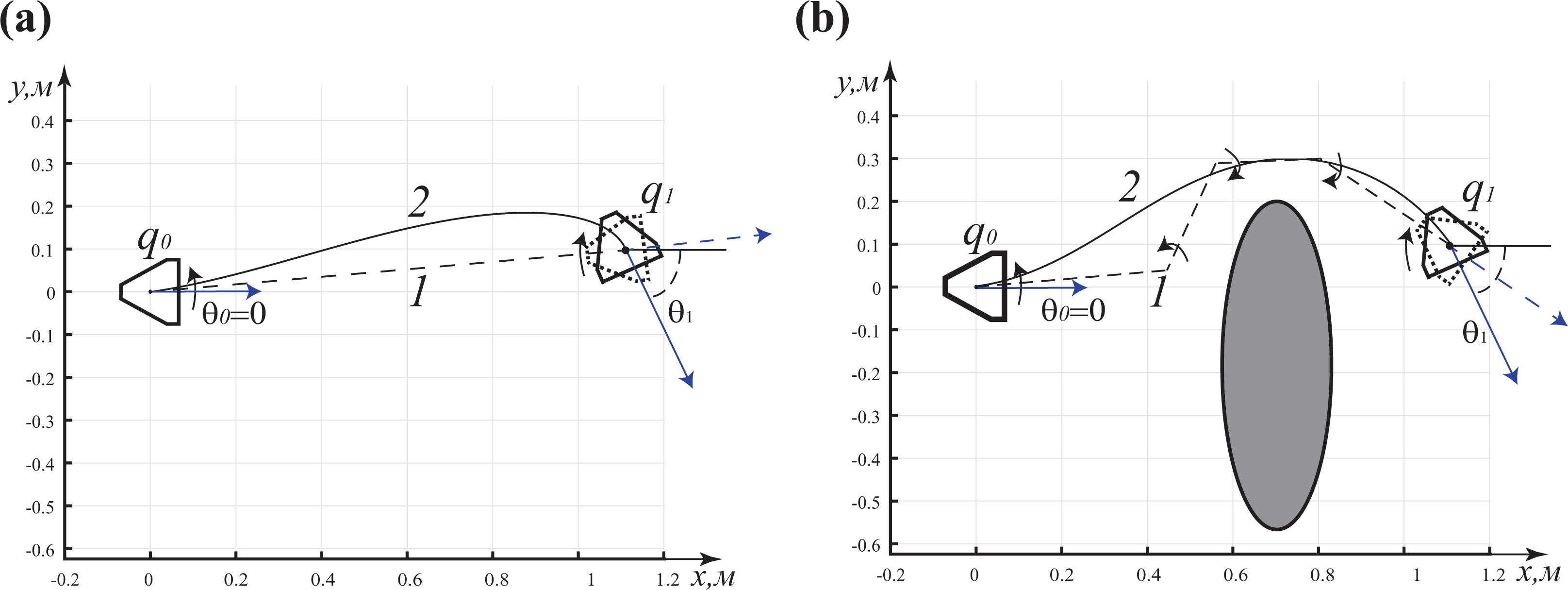
If the mobile robot encounters an obstacle in its path (see Figure 1(b)), its trajectory will become still more complex: a greater number of stops and additional turns will be required. When planning the path using continuous trajectories in the velocity, one can easily correct the trajectory of motion while ensuring the specified position and orientation at the end point (in this case, the trajectory is shown as a dashed line in Figure 1(b)). This solution is unique if the mobile robot has several links—passive trailers.
As continuous trajectories of motion, one can use approximations in the form of sinusoids, 3,4 polynomials, 14 –16 splines, 17,18 and trajectories in the form of Euler’s elastica. 19,20 However, all the abovementioned curves used as trajectories require rather lengthy calculations of their parameters. In our opinion, Euler’s elastica, which also ensures minimization of the control given by the difference of the angular velocity of rotation of the wheels, 21 holds the greatest promise. Trajectories in the form of Euler’s elastica can also be applied for multilink mobile robots.
The path planning algorithm which relates the initial and end points with the specified orientation of the mobile robot at the end point using Euler’s elastica is discussed in the study by Ardentov et al. 20 It is noted that the process of calculating the parameters of the elastica involves highly intensive computations, which can result in high costs for the control system of the mobile robot.
The purpose of this work is to search for an alternative solution to the complicated problem of calculating the parameters of Euler’s elastica. We suggest using ANNs as such a solution. Namely, using the data received from the sensors on the current position and velocity of the mobile robot and the point of destination specified by the coordinates
In this article, we propose a structure of the control system of the mobile robot. This structure is based on two ANNs, which are trained separately. One of them determines the data from the sensors, the position, and the size of the obstacle; and the other forms the parameters of the optimal trajectory of motion using these data and information on the point of destination and on the current position of the mobile robot. We also consider special features of the practical realization of the mobile robot, its control system, as well as algorithms for training neural networks.
The control of the mobile robot based on an ANN
Let us consider a modification of the control system where ANNs are applied for a prototype of the mobile wheeled robot with two driving wheels and one ball castor. A kinematic scheme and a three-dimensional model of the robot are shown in Figure 2. The driving wheels have a diameter of r 0 = 5 cm and are spaced l 0 = 24 cm from each other. In addition, their axes of rotation coincide, and the ball castor is equidistant from them.

A prototype of the mobile wheeled robot: (a) a kinematic scheme and (b) a three-dimensional model.
The electric motors and the incremental encoders are located on the same axis as the wheels. This design makes it possible to define and estimate the angular velocity of one driving wheel independently of each other.
To control the mobile wheeled robot along optimal trajectories connecting its initial and final positions, taking into account the obstacles encountered in its path, a control system based on ANNs has been developed. The general structural scheme of the control system of the mobile wheeled robot is presented in Figure 3.
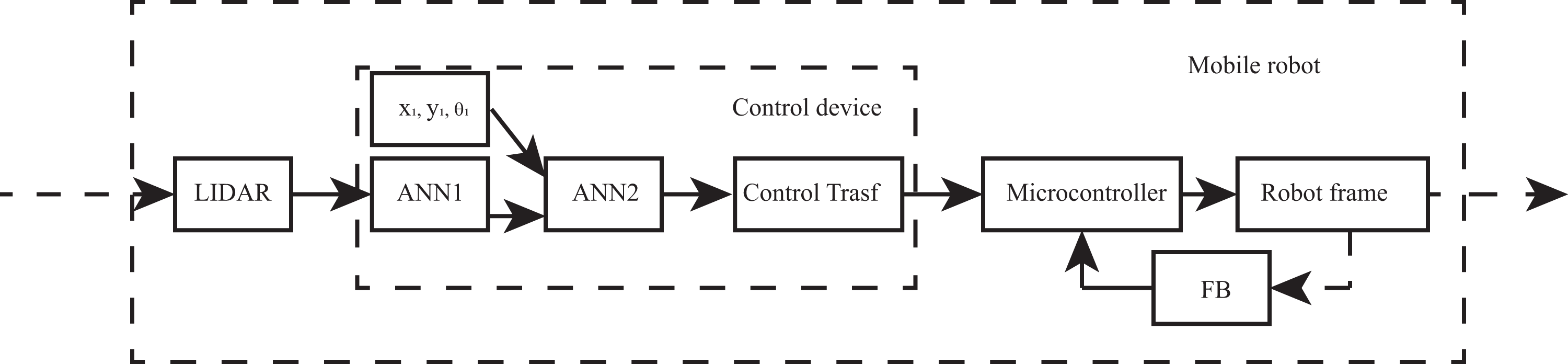
A generalized structural scheme of the control system.
The control system includes two ANNs and a unit for formation of commands for the onboard microcontroller of the robot (Control Transf). The system has been divided into two neural networks for ease of training and for their separate use in the future. Technically, the control system unit can be realized on a stationary personal computer or in the cloud to accelerate the process of training the network using a large amount of simulated data. In this case, the transfer of data on the environment and control actions to the microcontroller of the onboard control system is performed via a wireless communication channel.
The control system of the mobile robot receives data on the environment from the laser scanner (Lidar). These data are information on the distance to the surrounding objects or on their absence in the path of the robot. The structure of ANN1 is shown in Figure 4. The data coming from the Lidar sensor are a vector consisting of 360 values, which correspond to the distances to the surrounding objects around the robot with a discreteness of 1°. The data refresh rate depends on the operation speed of the laser scanner. The experiments were conducted for a laboratory prototype with the laser scanner RPLidar A1, which has a refresh rate of 5 Hz.
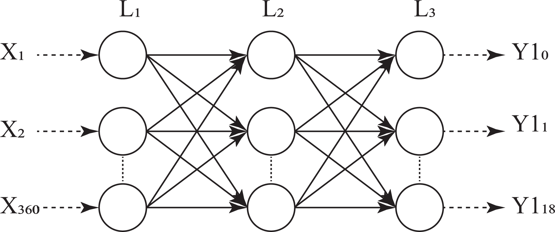
Structure of ANN1. ANN: artificial neural network.
The ANN1 has three layers. The number of neurons in the first layer is 360, which corresponds to the dimension of the input vector containing information on distances to the surrounding objects. The second is an intermediate layer which also contains 360 neurons, and the third is an output layer containing 18 neurons. The output neurons encode the coordinates of the obstacle

Graphical representation of the data obtained from the Lidar sensor.
For objects having more complicated form, ANN1 also formed three parameters: the radius of the circumscribed circle and the coordinates of its center. These values suffice to form a trajectory required for the robot to take a detour around the obstacle.
The second ANN2 (see Figure 6) also has three layers. The first layer of ANN2 has 6 neurons, the second also 6, and the output layer has 24 neurons, which encode the parameters of the elastica,
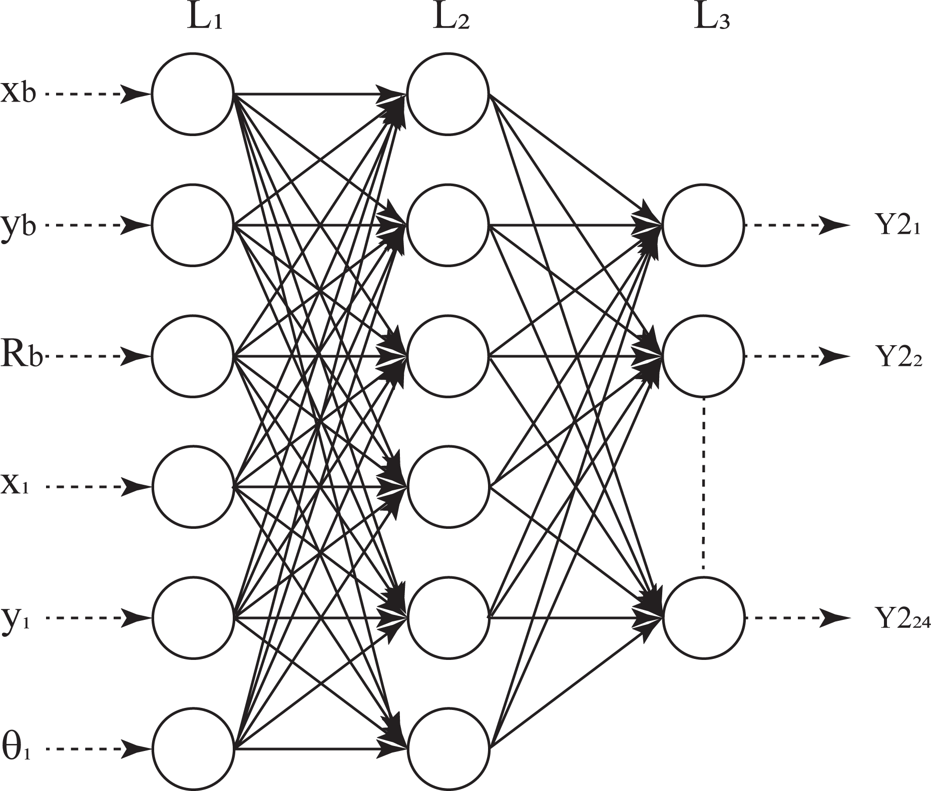
Structure of ANN2. ANN: artificial neural network.
Formation of optimal trajectories
The kinematics of the motion of the mobile wheeled robot with a differential drive and a ball castor is described by the following system of differential equations:
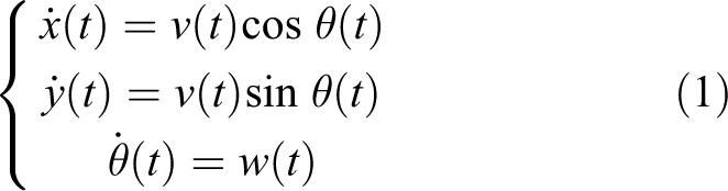
where t is the time parameter,
The solution to the system of equation (1) can be found in the class of optimal controls of continuous functions, called Euler’s elastica, 21 which are described by the following equations

where s is the length of the trajectory, symbol “′” denotes the derivative with respect to s, and
Euler’s elastica ensures local minimization of the squared curvature (control) 21

It is convenient to realize the relation between the angular velocity and the curvature of the trajectory by introducing the parameter defining smooth motion along the trajectory

Then, it is convenient to divide the trajectory of motion into three segments: acceleration from rest, motion with maximal velocity, and smooth stop

where vb
, vm
, and ve
are the velocities of motion on the corresponding segments, and
A graphical representation of changes in the velocity during motion along Euler’s elastica is shown in Figure 7 for

An example of the functions

The lengths of the corresponding time intervals are

Using the reparameterization (4)–(6), we obtain

The curvature of the elastica is defined in terms of elliptic Jacobi functions (
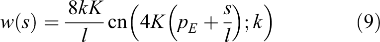
where
The second type includes noninflexional elasticas, which are calculated in accordance with the expression

and differ from the inflexional elasticas in that they have no inflexion points. Examples of inflexional and noninflexional elasticas are given in Figure 8.

Examples of Euler’s elasticas: (a) inflexional elasticas and (b) noninflexional elasticas.
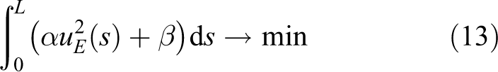
The above analysis allows the conclusion that the key parameters defining the trajectory of motion in the form of Euler’s elastica are the parameters


with a fixed value of L for the system (8) with a global minimization of the functional
where
Formation of controls for implementation of the motion of the mobile robot along optimal trajectories
We describe an algorithm for forming control actions to implement motion from an arbitrary initial position
1. Denote the distance on the plane between the initial and final positions by

from which we calculate the parameters for an optimal elastica of the length

namely, the values of
2. Construct elasticas of equal or smaller length for the resulting value of the maximal length of the elastica, L; calculate the values of the integral (13) from the parameter values of these elasticas. The parameters ensuring minimization of the integral are used later to calculate the angular velocities.
3. Calculate the linear and angular velocities
4. Calculate, from the values obtained for

where
Using relation (4), one can rewrite the integral (13) in terms of the linear and angular velocities of the robot

We note that, when

5. The resulting values of the angular velocities are transmitted to the control system, which regulates them by means of feedback sensors.
This algorithm was used to model and form teaching sets for training the ANN2.
Training of a neural network control system
The implementation of the ANNs, their training, and testing were carried out using the framework “TensorFlow.”
23
For the training of the networks, we used the method of gradient descent with back propagation of error. To prepare teaching samples for ANN1, we developed a program that simulates the environment, that is, randomly generates objects—obstacles having different sizes and different locations. To reduce the training time, we considered only cases where the obstacles were in the following intervals: the position of the obstacle
To train ANN2, the teaching samples were formed for different coordinates of the point of destination

Examples of inflexional Euler elasticas. Coordinates of the end points: (a)
Experiments
After the training of ANN1 and ANN2, two natural experiments were conducted in which the mobile robot moved to the point with coordinates (1.3; −0.5 m) and the orientation angle 0.13 rad. One of the experiments was carried out with an obstacle in the path of the mobile robot (see Figure 10) and without an obstacle (see Figure 11).

Experimental and theoretical trajectories of the mobile wheeled robot with an obstacle in its path. The dashed line indicates the theoretical trajectory, and the solid line corresponds to the experimental trajectory obtained during control using the neural network.

Experimental and theoretical trajectories of the mobile wheeled robot without an obstacle in its path. The dashed line indicates the theoretical trajectory, and the solid line corresponds to the experimental trajectory obtained during control using the neural network.
Experimental trajectories were fixed by cameras of a motion capture system Vicon. A cylindrical object with diameter 9 cm and coordinates (0.41; −0.28) was used as an obstacle. The resulting trajectories showed that at the end points, the difference of the trajectories obtained in the natural experiments from the theoretical trajectories does not exceed 1 cm with a trajectory length of 1.5 m. This error is due to random errors such as the accuracy of the position of the mobile robot at the start, surface irregularities, and inaccuracies in determining the parameters of the mobile robot. On the whole, the algorithm has shown its efficiency.
Conclusions
The results of the natural experiments confirm the efficiency of the proposed control algorithm for the mobile robot to move to the point with a given position and a given orientation. The training of the mobile wheeled robot to move along predetermined trajectories in the form of Euler’s elastica will ensure an optimal control and reduce the training time as compared to the training based only on experimental data. For the future, it is planned to increase the base of teaching samples, teach ANN to use a larger number of trajectories, and check the performance capability of its control. It is also planned to extend the existing functional of ANN to include the possibility of taking detours around dynamical obstacles and to perform reinforcement learning.
Footnotes
Declaration of conflicting interests
The author(s) declared no potential conflicts of interest with respect to the research, authorship, and/or publication of this article.
Funding
The author(s) disclosed receipt of the following financial support for the research, authorship, and/or publication of this article: The work of Pavol Bozek and Yuriy L Karavaev (sections 1, 3, 5, and 7) was funded by research project VEGA 1/0019/20 and by the RFBR grant 18-38-00454 mol_a, and is sponsored by the project 015STU-4/2018. The reported study of Andrey A Ardentov (Formation of optimal trajectories) was funded by RFBR, project number 19-31-51023 and was carried out at the Sirius University of Science and Technology (Sochi, Russia) and Ailamazyan Program Systems Institute of RAS (Pereslavl-Zalessky, Russia), and the work of Kirill S Yefremov (sections 2 and 6) was carried out within the framework of the project of the State Assignment at the Kalashnikov Izhevsk State Technical University under grant no 1.2405.2017/4.6.