A G 2 Continuous Path-smoothing Algorithm Using Modified Quadratic Polynomial Interpolation

Abstract

Path searching algorithm is one of the main topics in studies on path planning. These algorithms are used to avoiding obstacles and find paths from starting point to target point. There are dynamic problems that must be addressed when these paths are applied in real environments. In order to be applicable in actual situations, the path must be a smooth path. A smooth path is a path that maintains continuity. Continuity is decided by the differential values of the path. In order to be G² continuous, the secondary differential values of the path must be connected throughout the path. In this paper, the interpolation method is used to construct continuous paths. The quadratic polynomial interpolation is a simple method for obtaining continuous paths about three points. The proposed algorithm makes a connection of three points with curves and the proposed path is rotated using the parametric method in order to make the path optimal and smooth. The polynomials expand to the next three points and they merge into the entire path using the membership functions with G² continuity.

1. Introduction

Path planning is an important topic in robotics studies. One of the general purposes of path planning is to construct collision free paths. Typical approaches include the D^* algorithm [1], the Probabilistic Roadmap Method (PRM) algorithm [2], the Rapidly-exploring Random Tree algorithm (RRT) [3], and the potential field algorithm [4]. These algorithms can construct collision free paths, but they cannot guarantee that the resulting paths will be able to apply driving with stability and optimality in real environments.

Collision free paths are designed for obstacle avoidance. However, a continuous path is also suitable for the actual movements of robots. The actual movements of robots are affected by various forces (i.e., gravity, centrifugal force and centripetal force). These forces contribute to dynamic problems such as the slip and over-actuation of wheels, limitations of velocity and acceleration, and the effects of inertia. The forces that affect real movements need to be taken into consideration when planning and improving paths.

Considering these forces, paths should be continuous paths. There are paths connecting points on a two dimensional plane. Continuity is defined using geometry [5]. A G⁰ continuous path is simply a path that is connected for entire sections. These paths can be constructed by the path searching algorithms mentioned above. A G¹ continuous path matches the primary differential values at each point. This path shares a common tangent direction. A G² continuous path has the same secondary differential values at each point. This path also shares a common centre of curvature. Hence, a Gⁿ continuous path signifies the equality of the n^th differential value at each point.

The primary differential values on the paths indicate velocity. In addition, the secondary difference values indicate acceleration. Thus, the G¹ continuous paths have continuous velocities. The G² continuous paths are guaranteed to have continuous accelerations. These can reduce dynamic problems.

In order to apply the mobile robot or vehicle, Suzuki et al. demonstrated smooth path planning with pedestrian avoidance for a wheeled robot [6]. Vaillagra et al. proposed smooth path and speed planning for smooth autonomous navigation [7]. Yang et al. reported a continuous curvature path-smoothing algorithm using cubic B zeir spiral curves for non-holonomic robots [8].

A continuous path is also called a smooth path and the construction of continuous path algorithms is defined as path smoothing algorithms. There are two kinds of path smoothing algorithms. The first type is a graphical method and the second is a functional method. The graphical method uses lines, arcs, circles and clothoids to construct smooth paths. It is possible to analyse the results from graphical methods. The Dubins method [9] is a typical method for doing this. The Dubins method finds the shortest curve that connects two points in the two dimensional plane using lines and arcs. This method can be expanded into another graphical method. However, methods such as these have problems with limitations on path expressions and discontinuities at junction points. In order to solve these problems, studies have focused on functional methods.

Functional methods use mathematical functions to express the path. These methods can be used to construct various types of paths. The spline interpolation method is widely used. This method finds functions for connections between two points using differential values at each point [10]. Komoriya et al. suggested the B-spline method for designing trajectory and controlling wheel-type mobile robots [11]. Magid et al. proposed a spline-based method for robot navigation [12] and Piazzi et al. demonstrated smooth path generation using η splines for wheeled mobile robots [13]. The η spline method uses trigonometric functions and high order functions. Therefore, the complexities of the calculations increase and the numerical analysis can be complicated.

The polynomial interpolation method [5] is a simple functional method. This method finds a polynomial that includes all of the points. The number of points that are needed to construct a (n – 1) ^th order polynomial is n. Polynomials can be used to find simple methods for constructing paths. However, high order polynomials lead to the Runge's phenomenon [14] and a sharp increase in computation.

The essential requirements of a path smoothing algorithm are as follows: it must be possible to obtain the path using simple methods and calculations; the functions should be expressed in differential form; G² continuity must be maintained throughout the proposed path; it must be possible to express the vertical and horizontal path; it must be able to obtain the heading angle and curvature in order to enable analysis of the planned path.

To satisfy these requirements, this paper used a functional method. The spline interpolation method is used to form connections between points. These connections were suitable for the path smoothing algorithm using the start point (SP), the way points (WP) and the target point (TP) (these points are the position that robots or vehicles must visit on the map). They are also suitable for converting paths from line connecting paths to smooth paths. However, the trigonometric functions and high order functions can be used with the advanced spline interpolation method [13]. These functions lead to a high level of complexity. It is possible to use the polynomial interpolation method for the smoothing algorithm along with the necessary requirements. However, the polynomial method does not give an optimal path for random points. Also this method cannot be used many WPs, because Runge's phenomenon can occur. Additionally, high order polynomials increase the calculation load.

Spline interpolation methods and polynomial interpolation methods can be used to interpolate a graph of the geometry. These methods should be used with the variations of x or y. The x or y values are always increased or decreased in order to obtain the functions by general polynomial interpolation methods (Newton's polynomial interpolation and Lagrange's polynomial interpolation) [5]. Therefore, general polynomial interpolation methods cannot express vertical or horizontal movements like those of robots and vehicles.

In this paper, the polynomial interpolation method is used. If the x or y values of points are located at equal distances, the quadratic polynomial is the minimum order polynomial that includes three points with G² continuity. However, another method is required in order to express a path of irregular points or a path of points that has the same value on axis. It is possible for the rotated polynomials to give the shortest and continuous path for three points; however, it is difficult to obtain the rotated polynomials using normal methods. The general rotation method uses a rotation matrix. This matrix relies on trigonometric functions and can therefore lead to complex calculations. In this paper, the parametric method is used to obtain the rotated polynomials.

To apply for three or more points, the quadratic polynomial is extended to the subsequent three points and they are combined with the previous polynomial. Therefore, the proposed method should be able to construct a G² continuous polynomial that includes the next three points using the quadratic polynomial. In this paper, the membership function is used to combine polynomials. The membership function is part of a fuzzy algorithm. This function is used to regulate the certainty of a fuzzy set. The proposed method uses the membership function for distributing the degree of the polynomials in the overlapping sections. The fuzzy set assumes the polynomials and the membership function is changed based on the accumulation value of the linear distance. This function controls the degree of each polynomial. Thus, the n^th polynomial has the maximum degree at the n^th WP, but this degree decreases closer to the (n + 1) ^th WP. The (n + 1) ^th polynomial has the minimum degree at the n^th WP. This degree increases closer to the (n + 1) ^th WP. Hence, the polynomials are combined by the membership function controlling degree at each WP.

This paper is organized as follows: section 2 explains the characteristics of quadratic polynomials and a conception of path smoothing using the quadratic polynomials. In section 3, the parametric method is proposed for constructing the rotated quadratic polynomials. Section 4 analyses the rotated quadratic polynomials. Section 5 describes how the membership function can be used to merge the polynomials. Section 6 reports the simulation results for the proposed path. Section 7 documents the conclusions.

2. Quadratic polynomial interpolation

2.1 Characteristics of quadratic polynomial

The quadratic polynomial is a second order function for connecting three points. If this function is used for the path, then the three points include the SP, WP and TP. If the WP is closer to the vertex, the path can be more appropriate for the shortest and continuous path.

In R², the quadratic polynomial is,

$\begin{array}{c}\mathbf{P}:(x,y)\in R^2\\ y=a{x}^2+bx+c\end{array}$

(1)

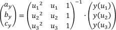
The quadratic polynomial connecting the three points (P₁:(x₁,y₁), P₂:(x₂,y₂) and P₃:(x₃,y₃)) can be obtained using the following method.

$\begin{array}{c}\left(\begin{array}{c}{y}_1\\ y_2\\ y_3\end{array}\right)=\left(\begin{array}{ccc}{x_1}^2& x_1& 1\\ {x_2}^2& x_2& 1\\ {x_3}^2& x_3& 1\end{array}\right)·\left(\begin{array}{c}a\\ b\\ c\end{array}\right)\\ \left(\begin{array}{c}a\\ b\\ c\end{array}\right)={\left(\begin{array}{ccc}{x_1}^2& x_1& 1\\ {x_2}^2& x_2& 1\\ {x_3}^2& x_3& 1\end{array}\right)}^{-1}·\left(\begin{array}{c}{y}_1\\ y_2\\ y_3\end{array}\right)\end{array}\hspace{0.17em}$

(2)

If (3) and (4) are satisfied, the graph of (1) is shown in Figure 1.

$\left|x_1-x_2\right|=\left|x_2-x_3\right|$

(3)

$y_1=y_3$

(4)

Figure 1.

Graph of quadratic polynomial ((1) with (3) and (4))

In Figure 1, the graph can have one of two forms depending on the values of y₁, y₂ and y₃. This graph is unique and satisfies G² continuity.

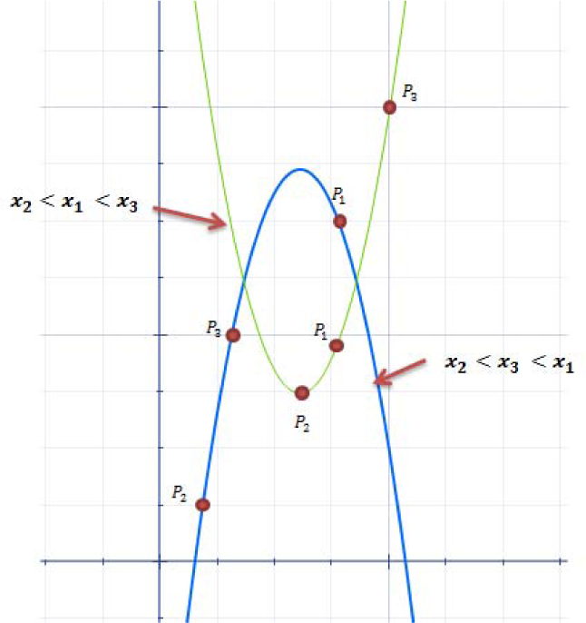
If (3) and (4) are not satisfied, then P₂ is not the vertex. The resulting graph is shown in Figure 2.

Figure 2.

Graph of quadratic polynomial ((1) without (3) and (4))

The quadratic polynomial can be obtained from (1) depending on the location of the point. In the case of #1 (green curve) in Figure 2, P₁ is the vertex between P₂ and P₃. However, in the case of #2 (blue curve) in Figure 2, P₁, P₂ and P₃ are not sequential. This path can be a distorted path. Therefore, constraints (3) and (4) must be satisfied to obtain the shortest and continuous path with G² continuity in the general quadratic polynomial.

If constraints (3) and (4) do not hold or points P₁ P₂ and P₃ are not sequential (5), the quadratic polynomial cannot be obtained for the following condition: (x_n = x_n+1). The values of x must have variation. These constraints mean that general polynomial interpolation cannot apply to the path smoothing algorithm.

$x_1>x_2>x_3\mathrm{\hspace{0.17em}}or\mathrm{\hspace{0.17em}}{x}_1<x_2<x_3$

(5)

2.2 Shortest and continuous path using quadratic polynomial

If the points do not satisfy constraint (5), then the values of x are not sequential or the values of y have not changed. Figure 3 shows the graph of the polynomial for an irregular x. Points P₁, P₂ and P₃ are located irregularly on the curve.

Figure 3.

Graph of quadratic polynomial with irregular x

The simple method (2) can be used to construct the quadratic polynomial that connects P₁, P₂ and P₃. However, it is impossible to use this method to produce a sequential path that connects P₁, P₂ and P₃. Furthermore, the other general methods (Lagrangian interpolation polynomials and Newton's interpolation polynomials) [5] require the variation of x or y. The path cannot be constructed using these methods for the following conditions: x₁ = x₂, x₂ = x₃, y₁ = y₂ and y₂ = y₃. These conditions occurred for vertical and horizontal movements on the 2D-plane.

The shortest and continuous path for irregular values of x is shown in Figure 4.

Figure 4.

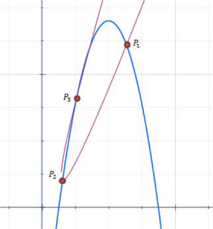
Graph of optimal path with irregular values for x (red curve)

The red curve is the shortest curve centred on P₂ (middle point) and includes P₁, P₂ and P₃. This curve is constructed using the quadratic polynomial. In this paper, this red curve is used to construct the smooth path with continuity.

3. Modified quadratic polynomial interpolation using the parametric method

In section 2, the quadratic polynomial graph is centred on P₂ and is rotated. However, (1) is changed by the rotation matrix, which is based on the trigonometric functions that are used to construct the rotated quadratic polynomial [15]. The trigonometric functions are occurred complex calculations and open sections. Vertical and horizontal paths cannot be constructed using the trigonometric functions. The key characteristics of trigonometric functions are that tanθ has an unlimited value at $\theta =\frac{\pi }{2}$ and $\theta =\frac{3\pi }{2}$ .

In this paper, a parameter u is used. The parameter u is the linear distance between each point. u₁ is always zero. u₂ is the distance between P₁ and P₂. u₃ can be obtained by calculating u₂ and the distance between P₂ and P₃. The functions are as follows:

$\begin{array}{c}{u}_1=0\\ u_2=u_1+\sqrt{{\left(x_2-x_1\right)}^2+{\left(y_2-y_1\right)}^2}\\ {\hspace{0.17em}\hspace{0.17em}u}_3=u_2+\sqrt{{\left(x_3-x_2\right)}^2+{\left(y_3-y_2\right)}^2}\end{array}$

(6)

(1) can be transformed into (8) and (9) using u.

$\mathbf{P}:\left(x\left(u\right),y\left(u\right)\right)$

(7)

$x\left(u\right)=a_x{u}^2+b_{x}u+c_x$

(8)

$y\left(u\right)=a_y{u}^2+b_{y}u+c_y$

(9)

Equations (8) and (9) are the quadratic polynomials of u. The parameter u always has a positive value and connects each point in the serial order with irregular x and y values. The function of x is changed to the function of u. The function of u is seperate from that of x and y. Each of the functions has the same characteristics and the continuity that is derived from the quadratic polynomial.

Equation (2) can be transformed into (10) and (11) using the u parameter.

$\left(\begin{array}{c}{a}_x\\ b_x\\ c_x\end{array}\right)={\left(\begin{array}{ccc}{u_1}^2& u_1& 1\\ {u_2}^2& u_2& 1\\ {u_3}^2& u_3& 1\end{array}\right)}^{-1}·\left(\begin{array}{c}x\left(u_1\right)\\ x\left(u_2\right)\\ x\left(u_3\right)\end{array}\right)$

(10)

$\left(\begin{array}{c}{a}_y\\ b_y\\ c_y\end{array}\right)={\left(\begin{array}{ccc}{u_1}^2& u_1& 1\\ {u_2}^2& u_2& 1\\ {u_3}^2& u_3& 1\end{array}\right)}^{-1}·\left(\begin{array}{c}y\left(u_1\right)\\ y\left(u_2\right)\\ y\left(u_3\right)\end{array}\right)$

(11)

Equation (12) is a generalized from of equation (6). The m parameter represents the number of points.

$\begin{array}{c}{u}_1=0\\ u_n=\sum _{n=2}^m\sqrt{{\left(x_n-x_{n-1}\right)}^2+{\left(y_n-y_{n-1}\right)}^2}\end{array}$

(12)

Equations (10) and (11) can be generalized to:

$\left(\begin{array}{c}{a}_{x_{n-1}}\\ b_{x_n}\\ c_{x_{n+1}}\end{array}\right)={\left(\begin{array}{ccc}{u_{n-1}}^2& u_{n-1}& 1\\ {u_n}^2& u_n& 1\\ {u_{n+1}}^2& u_{n+1}& 1\end{array}\right)}^{-1}·\left(\begin{array}{c}{x}_n\left(u_{n-1}\right)\\ x_n\left(u_n\right)\\ x_n\left(u_{n+1}\right)\end{array}\right)$

(13)

$\begin{array}{c}\left(\begin{array}{c}{a}_{y_{n-1}}\\ b_{y_n}\\ c_{y_{n+1}}\end{array}\right)={\left(\begin{array}{ccc}{u_{n-1}}^2& u_{n-1}& 1\\ {u_n}^2& u_n& 1\\ {u_{n+1}}^2& u_{n+1}& 1\end{array}\right)}^{-1}·\left(\begin{array}{c}{y}_n\left(u_{n-1}\right)\\ y_n\left(u_n\right)\\ y_n\left(u_{n+1}\right)\end{array}\right)\\ (2\le n\le m-1)\end{array}$

(14)

Equations (8) and (9) are described as follows:

$x_n\left(u\right)=a_{x_n}{u}^2+b_{x_n}u+c_{x_n},\mathrm{\hspace{0.17em}}(2\le n\le m-1)$

(15)

$y_n\left(u\right)=a_{y_n}{u}^2+b_{y_n}u+c_{y_n},\mathrm{\hspace{0.17em}}(2\le n\le m-1)$

(16)

Equation (7) is defined based on (17).

$\mathbf{P}\left(u\right)=\left\{\begin{array}{c}\left(x_2\left(u\right),\mathrm{\hspace{0.17em}}{y}_2\left(u\right)\right),\hspace{0.17em}(u_1\le u_2\le u_3)\\ \left(x_3\left(u\right),\mathrm{\hspace{0.17em}}{y}_3\left(u\right)\right),(u_2\le u_3\le u_4)\\ ⋮\\ \left(x_{m-1}\left(u\right),\mathrm{\hspace{0.17em}}{y}_{m-1}\left(u\right)\right),(u_{m-2}\le u_{m-1}{\le u}_m)\end{array}\right.$

(17)

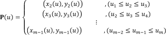
x_n(u) and y_n(u) are the quadratic polynomials that are connected by three points with u. They are the parametric quadratic polynomials of (P₁,P₂,P₃), (P₂,P₃,P₄),⋯,(P_m-2,P_m-1,P_m).

If there are 5 points, P₁, P₂, P₃, P₄ and P₅ then P₁ is SP, P₂ to P₄ are WPs, and P₅ is TP. x₂(u) and y₂(u) consist of P₁, P₂ and P₃. x₃(u) and y₃(u) are obtained from P₂, P₃, and P₄. x₄(u) and y₄(u) can be obtained by the same method.

In Figure 5, the blue curve is P(x₂(u),y₂(u)) and it connects P₁, P₂ and P₃ in serial order. P(x₃(u),y₃(u)) is expressed by the red curve. The green curve shows P(x₄(u),y₄(u)). There are overlapping sections in P₂ to P₃ and P₃ to P₄. The smoothing algorithm for these sections will be described in section 5.

Figure 5.

Graph of quadratic polynomials using a parametric method with 5 points

4. Analysis of quadratic polynomial

The primary and secondary differential values of (1) are described as follows:

$y^{\prime }=2ax+b$

(18)

$y^{″}=2a$

(19)

The curvature of (1) can be obtained using (18) and (19).

$k=\frac{y^{″}}{{(1+{y^{\prime }}^2)}^{\frac{3}{2}}}=\frac{2a}{{\left({\left(2ax+b\right)}^2+1\right)}^{\frac{3}{2}}}$

(20)

Equations (8) and (9) can be differentiated using u.

$\frac{dx}{du}=2a_{x}u+b_{x\prime }\frac{d^{2}x}{d{u}^2}=2a_x$

(21)

$\frac{dy}{du}=2a_{y}u+b_{y\prime }\frac{d^{2}y}{d{u}^2}=2a_y$

(22)

The curvature of the parametric quadratic polynomial can be described as follows:

$k=\frac{|x^{\prime }{y}^{″}-y^{\prime }{x}^{″}|}{{({x^{\prime }}^2+{y^{\prime }}^2)}^{\frac{3}{2}}}$

(23)

The primary differential function is a function of u. The secondary differential function takes on a constant value. The general quadratic polynomial (that connects only three points) has the same primary and secondary differential values at each point. Therefore, each polynomial has G² continuity as those in (21) and (22).

The heading angles of mobile robots and vehicles are defined as follows:

$\theta ={\tan }^{-1}\left(\frac{y\prime }{x\prime }\right)={\tan }^{-1}\left(\frac{2a_{y}u+b_y}{2a_{x}u+b_x}\right)$

(24)

The heading angles are important data for path analysis and driving. The primary differential values of x and y can be used to obtain these values (24).

However, the method for finding continuity and heading angles cannot be applied to the overlapping sections. Section 5 describes the method for finding these values in the overlapping sections.

5. Modified quadratic polynomial interpolation using the parametric method and membership function

5.1 Membership function

The membership function is used to control the degree of truth in the fuzzy control theory.

The membership function μ(x) increases from 0 to 1 as x increases. μ(x) starts at 0 and increases to 1 until the centre of x. This function decreases to 0 again as x increases. In this paper, the membership function is used to control the degree of each polynomial's effect on the entire path. In Figure 6, x is changed to u and the membership function is extended to the m ^th membership functions, as shown in Figure 7.

Figure 6.

Membership function of a fuzzy set (triangle)

Figure 7.

Graph of membership functions vs. u

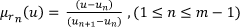
The membership function of n^th has two types, a rising function and a falling function. The dotted lines in Figure 7 represent the rising function. This function has increased from 0 to 1 for the u_n-1_to u_n section. The falling function is represented by the dashed lines in Figure 7. This function has decreased 1 to 0 for the u_n to u_n+1 section. General function can be described as follows:

${{\mu }_r}_n\left(u\right)=\mathrm{\hspace{0.17em}}\frac{\left(u-u_n\right)}{{(u}_{n+1}-u_n)}\mathrm{\hspace{0.17em}},(1\le n\le m-1)$

(25)

${{\mu }_f}_n\left(u\right)=\mathrm{\hspace{0.17em}}\frac{\left(u_{n+1}-u\right)}{{(u}_{n+1}-u_n)}\mathrm{\hspace{0.17em}},\left(1\le n\le m-1\right)$

(26)

5.2 Polynomials and membership functions

P: (X(u), Y(u)) defines the group of the paths. These paths are constructed by combinations of the polynomials and membership functions. X(u) and Y(u) are described in (27) and (28) using (25) and (26).

$X(u)=\left\{\begin{array}{c}{{\mu }_r}_1\left(u\right)x_2\left(u\right)+{{\mu }_f}_1\left(u\right)x_1\left(u\right)\hspace{0.17em}:\hspace{0.17em}{u}_1\le u\le u_2\\ {{\mu }_r}_2\left(u\right)x_3\left(u\right)+{{\mu }_f}_2{\left(u\right)x}_2\left(u\right)\hspace{0.17em}:\hspace{0.17em}{u}_2\le u\le u_3\\ {{\mu }_r}_3\left(u\right)x_4\left(u\right)+{{\mu }_f}_3{\left(u\right)x}_3\left(u\right)\hspace{0.17em}:\hspace{0.17em}{u}_3\le u\le u_4\\ ⋮\\ {{\mu }_r}_{m-2}\left(u\right)x_{m-1}\left(u\right)+{{\mu }_f}_{m-2}\left(u\right)x_{m-2}\left(u\right)\hspace{0.17em}:u_{m-2}\le u\le u_{m-1}\\ {{\mu }_r}_{m-1}\left(u\right)x_m\left(u\right)+{{\mu }_f}_{m-1}{\left(u\right)x}_{m-1}\left(u\right)\hspace{0.17em}:u_{m-1}\le u\le u_m\end{array}\right.$

(27)

$Y(u)=\left\{\begin{array}{c}{{\mu }_r}_1{\left(u\right)y}_2\left(u\right)+{{\mu }_f}_1{\left(u\right)y}_1\left(u\right)\hspace{0.17em}:\hspace{0.17em}{u}_1\le u\le u_2\\ {{\mu }_r}_2{\left(u\right)y}_3\left(u\right)+{{\mu }_f}_2\left(u\right)y_2\left(u\right)\hspace{0.17em}:\hspace{0.17em}{u}_2\le u\le u_3\\ {{\mu }_r}_3\left(u\right)y_4\left(u\right)+{{\mu }_f}_3\left(u\right)y_3\left(u\right)\hspace{0.17em}:\hspace{0.17em}{u}_3\le u\le u_4\\ ⋮\\ {{\mu }_r}_{m-2}\left(u\right)y_{m-1}\left(u\right)+{{\mu }_f}_{m-2}\left(u\right)y_{m-2}\left(u\right)\hspace{0.17em}:u_{m-2}\le u\le u_{m-1}\\ {{\mu }_r}_{m-1}\left(u\right)y_m\left(u\right)+{{\mu }_f}_{m-1}\left(u\right)y_{m-1}\left(u\right)\hspace{0.17em}:u_{m-1}\le u\le u_m\end{array}\right.$

(28)

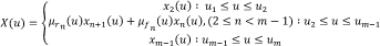
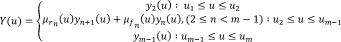
In the first section [P₁: P₂], the entire path consists of only (x₂(u),y₂(u)). In the last section [P_m-1:P_m], the entire path is constructed using only (x_m-1(u), y_m-1(u)). Therefore, μ_r1(u) and μ_fm-1(u) are always equal to 1.

$x_1\left(u\right)=x_m\left(u\right)=y_1\left(u\right)=y_m\left(u\right)=0$

(29)

${{\mu }_r}_1\left(u\right)={{\mu }_f}_{m-1}\left(u\right)=1$

(30)

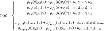
The general functions can be obtained by applying (29) and (30) to (27) and (28).

$X(u)=\left\{\begin{array}{c}{x}_2\left(u\right)\hspace{0.17em}:\hspace{0.17em}{u}_1\le u\le u_2\\ {{\mu }_r}_n\left(u\right)x_{n+1}\left(u\right)+{{\mu }_f}_n\left(u\right)x_n\left(u\right),\hspace{0.17em}(2\le n<m-1)\hspace{0.17em}:u_2\le u\le u_{m-1\mathrm{\hspace{0.17em}}}\\ x_{m-1}\left(u\right)\hspace{0.17em}:u_{m-1}\le u\le u_m\end{array}\right.$

(31)

$Y(u)=\left\{\begin{array}{c}{y}_2\left(u\right)\hspace{0.17em}:\hspace{0.17em}{u}_1\le u\le u_2\\ {{\mu }_r}_n\left(u\right)y_{n+1}\left(u\right)+{{\mu }_f}_n\left(u\right)y_n\left(u\right),\hspace{0.17em}(2\le n<m-1)\hspace{0.17em}:u_2\le u\le u_{m-1\mathrm{\hspace{0.17em}}}\\ y_{m-1}\left(u\right)\hspace{0.17em}:u_{m-1}\le u\le u_m\end{array}\right.$

(32)

Hence, the quadratic polynomial will be the cubic polynomial in each of the sections [P₂:P₃], [P₃,P₄], ⋯, [P_m-2, P_m-1]. In this paper, the proposed algorithm is concerned with finding the quadratic polynomial using irregular x and y. However, these polynimals are changed into the cubic functions by combining the membership functions. The graph of the overlapping sections has a curve representing the degree distribution based on the membership functions. The proposed method changes the path in Figure 5 into the path in Figure 8.

Figure 8.

Graph of the proposed method (dashed line)

5.3 Analysis of proposed path

To analyse the proposed path, the differential values should be obtained and checked. The primary differential value can be defined using (21), (22) and the membership functions. The primary differential values are decribed in (33) and (34).

$dX(u)=\left\{\begin{array}{c}d{x}_2\left(u\right)\hspace{0.17em}:\hspace{0.17em}{u}_1\le u\le u_2\\ {{\mu }_r}_n\left(u\right)d{x}_{n+1}\left(u\right)+{{\mu }_f}_n\left(u\right)d{x}_n\left(u\right),\hspace{0.17em}(2\le n<m-1)\hspace{0.17em}:u_2\le u\le u_{m-1\mathrm{\hspace{0.17em}}}\\ {dx}_{m-1}\left(u\right)\hspace{0.17em}:u_{m-1}\le u\le u_m\end{array}\right.$

(33)

$dY(u)=\left\{\begin{array}{c}d{y}_2\left(u\right)\hspace{0.17em}:\hspace{0.17em}{u}_1\le u\le u_2\\ {{\mu }_r}_n\left(u\right)d{y}_{n+1}\left(u\right)+{{\mu }_f}_n\left(u\right)d{y}_n\left(u\right),\hspace{0.17em}(2\le n<m-1)\hspace{0.17em}:u_2\le u\le u_{m-1\mathrm{\hspace{0.17em}}}\\ {dy}_{m-1}\left(u\right)\hspace{0.17em}:u_{m-1}\le u\le u_m\end{array}\right.$

(34)

The secondary differential values are described in (35) and (36).

$d^{2}X(u)=\left\{\begin{array}{c}{d^{2}x}_2\left(u\right)\hspace{0.17em}:\hspace{0.17em}{u}_1\le u\le u_2\\ {{\mu }_r}_n\left(u\right){d^{2}x}_{n+1}\left(u\right)+{{\mu }_f}_n\left(u\right)d^2{x}_n\left(u\right),\hspace{0.17em}(2\le n<m-1)\hspace{0.17em}:u_2\le u\le u_{m-1\mathrm{\hspace{0.17em}}}\\ d^2{x}_{m-1}\left(u\right)\hspace{0.17em}:u_{m-1}\le u\le u_m\end{array}\right.$

(35)

$d^{2}Y(u)=\left\{\begin{array}{c}{d^{2}y}_2\left(u\right)\hspace{0.17em}:\hspace{0.17em}{u}_1\le u\le u_2\\ {{\mu }_r}_n\left(u\right)d^2{y}_{n+1}\left(u\right)+{{\mu }_f}_n\left(u\right){d^{2}y}_n\left(u\right),\hspace{0.17em}(2\le n<m-1)\hspace{0.17em}:u_2\le u\le u_{m-1\mathrm{\hspace{0.17em}}}\\ d^2{y}_{m-1}\left(u\right)\hspace{0.17em}:u_{m-1}\le u\le u_m\end{array}\right.$

(36)

G¹ continuity is related to the matching of the primary differential value at each point and G² continuity is related to the agreement of the secondary differential value at each point. Each polynomial has the maximum degree at each point. Thus, x_n(u) and y_n(u) have the maximum degree at the n^th point. Therefore, the continuity at each point is decided by the differential values of x_n(u) and y_n(u). The values of x_n(u) and y_n(u) have G² continuity at the (n – 1) ^th , n^th and (n + 1) ^th points. The next set of polynomials, x_n+1(u) and y_n+1(u) are G² continuous at the n^th, (n + 1) ^th and (n + 2) ^th points. Hence, each polynomial has G² continuity. If these polynomials are combined using the membership functions, then G² continuity can be maintained throughout the entire path, because the membership functions distribute the degree of the polynomials and the differentials of the polynomials.

The heading angle can be obtained by modifying (24) using the primary differential values from (33) and (34).

$\theta ={\tan }^{-1}\left(\frac{dY\left(u\right)}{dX\left(u\right)}\right),\mathrm{\hspace{0.17em}}(2\le n<m-1)$

(37)

6. Simulations

6.1 Smooth path planning of random points

There are random points on the 2D-plane.

Table 1.

Random points for simulation

	P1(SP)	P 2	P 3	P 4	P 5	P 6	P 7	P 8	P 9	P10(TP)
x	8	7	2	11	11	45	45	25	12	25
y	5	15	10	10	14	30	12	45	45	25

The points of x and y have various values. P₄ and P₅ have the same x value. Also, P₈ and P₉ have the same y value. This means that the movement from P₄ to P₅ is a vertical movement and the movement from P₉ to P₁₀ is a horizonal movement.

The linear distance between the points can be obtained using (12). Table 2 displays a set of u values.

Table 2.

Set of u values

u 1	u 2	u 3	u 4	u 5
0	10.05	17.12	26.12	30.12
u 6	u 7	u 8	u 9	u 10
67.69	85.69	124.28	137.28	161.13

The variations of x and y can be changed into a function of u using (31) and (32). Figures 9 and 10 show the graphs of x and y vs. u.

Figure 9.

Graph of u vs. x

Figure 10.

Graph of u vs. y

The entire path that is shown in Figure 11 is based on (31), (32), Figure 9 and Fig 10.

Figure 11.

Smooth path of random points based on the proposed method

The proposed path is a continuous curve. To verify the continuity, the primary differential values should be checked. The primary differential values are obtained using (33) and (34). Figures 12 and 13 display the graphs of the primary differential values.

Figure 12.

Graph of u vs. dx

Figure 13.

Graph of u vs. dy

The dx and dy values are connected throughout each of the graphs. The connectedness of the primary differential values signifies that the proposed path is G¹ continuous.

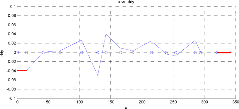
The status for G² continuity can be decided by checking the secondary differential values. These values can be obtained using (35) and (36). The graphs are as follows:

Figures 14 and 15 display the secondary differential values of proposed path. The values are also connected throughout each of these graphs. These graphs demonstrate that the path has G² continuity.

Figure 14.

Graph of u vs. d²x

Figure 15.

Graph of u vs. d²y

The curvature graph is shown in Figure 16. The curvature can be obtained using (23).

Figure 16.

Graph of u vs. curvature

The heading angle graph that is shown in Figure 17 is based on (37).

Figure 17.

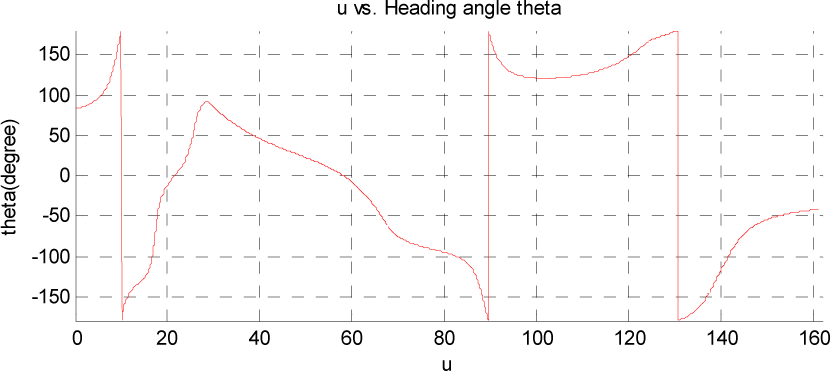
Graph of u vs. heading angle

The heading angle and curvature can be applied to the analysis of the planned path.

This simulation shows that the proposed method can be used to construct G² continuous paths. This method can also use for the analysis of paths with random points.

6.2 Path smoothing of PRM planner planned path

Figure 18 shows a path from the PRM planner [16]. This planner is used to construct collision free G⁰ continuous paths. In this simulation, the proposed method will be applied to the planning process for G⁰ continuous paths in order to improve continuity.

Figure 18.

Path from the PRM algorithm (bold line)

The variation of x and y are shown in Figures 19 and 20.

Figure 19.

Graph of u vs. x

Figure 20.

Graph of u vs. y

The functions of x and y are the increased functions with respect to u. To show the entire path, Figures 19 and 20 are combined to produce Figure 21.

Figure 21.

Path with improved continuity based on the proposed method

Each of the functions is G² continuous. It is necessary to check the differential values in order to verify continuity. Figures 22–25 are the graphs of the differential values.

Figure 22.

Graph of u vs. dx

Figure 23.

Graph of u vs. dy

Figure 24.

Graph of u vs. d²x

Figure 25.

Graph of u vs. d²y

Figures 22 and 23 prove that the differential values are connected.

The secondary differential values do not have any open sections. These figures indicate that the proposed path is also G² continuous.

The curvature and heading angle are shown in the following graphs:

Figures 26 and 27 demonstrate that it is possible to analyse the proposed path.

Figure 26.

Graph of u vs. curvature

Figure 27.

Graph of u vs. heading angle

In this simulation, the proposed method was used to improve a G⁰ continuous path so that it was also G² continuous. The differential values, curvature and heading angle were also obtained. These values show that the proposed method can be used to construct continuous and analysable paths.

7. Conclusions

Continuous paths are important for driving mobile robots and vehicles in real environments. The spline interpolation method and polynomial interpolation methods have problems with tasks involving expressing and analysing paths. In this paper, the quadratic polynomial interpolation method was used to construct a G² continuous path. The quadratic polynomial can easily be obtained using a simple matrix. The proposed method is based on the rotated quadratic polynomial. This polynomial gives the shortest path with G² continuity and also the minimum order. To express the rotated quadratic polynomial, the parametric method was used. This method uses an accumulated linear distance value u. The variations of x and y values are transformed into functions of u. The polynomials of x and y can be expressed using the polynomial interpolation method. These functions are always increasing and make it possible to express vertical and horizontal movements. However, it is possible to use the proposed method only if there are three points. To apply the proposed method for three or more points, the membership functions are used to distribute the degrees of polynomials in overlapping sections. The quadratic polynomials are combined with the membership functions, which affect the whole path because of variations in the membership functions.

The differential values are obtained using the differential functions of x and y. These values can be used to prove the continuity of path and can also serve as the basis for the curvature and heading angle.

Simulation results show that proposed methods can construct a G² continuous path with WPs. The first simulation constructed a G² continuous path with ramdom points. The second simulation demonstrated that the proposed algorithm can be applied directly to the searched path from the PRM algorithm.

In order to use a real robot navigation system, the searched paths have WPs, or they are G⁰ continuous paths. PRM algorithm planned path can change directly, as shown in the simuilation. However, the D^* algorithm and potential field algorithm requires another algorithm to decide WPs.

If there are WPs and a sequential rule of visiting WPs, the proposed method can construct a G² continuous path using only a second order polynomial. In addition, this method is a new interpolation method. It is not a required database for saving entired path. Additionally, the proposed method can use local path planning. In local path planning, if mobile robots or vehicles know the following two WPs, the proposed method can construct a G² continuous path of three points. In addition, if robots or vehicles reach the next point, the proposed method can update the paths using the reached point and the next two points.

This study suggests simple methods for obtaining G² continuous paths using analysable and functional forms. This research can be applied to the path smoothing algorithm and the curve fitting algorithm for G² continuity. If the proposed method is extended to 3D-space, it can be applied to flying robots and aircraft.