
Abstract
In this paper, the global finite-time stabilization problem is considered for nonholonomic mobile robots based on visual servoing with uncalibrated visual parameters, control direction and unmatched external disturbances. Firstly, the simple dynamic chained-form systems is obtained by using a state and input transformation of the kinematic robot systems. Secondly, a new discontinuous switching controller is presented in the presence of uncertainties and disturbances, it is rigorously proved that the corresponding closed-loop system can be stabilized to the origin equilibrium point in a finite time. Finally, the simulation results show the effectiveness of the proposed control design approach.
Keywords
Introduction
Addressing the stabilization problem of nonholonomic systems is a challenging task which has attracted a continuously increasing attention in the control community. As pointed out in [1], such a class of nonlinear systems can not be stabilized to a point with pure smooth (or even continuous) state feedback control. To overcome this difficult, up to now, there have been a lot of control methods to stabilize such systems, which includes discontinuous feedback control laws [2]–[5], continuous time-varying feedback control laws [6]-[8] and hybrid feedback control laws [9]-[11]. As a typical model of the nonholonomic system, the nonholonomic characteristic of wheeled mobile robots arises from the wheel which is rolling without slipping. Many research results of controlling nonholonomic mobile robots have been given in recent decades, such as formation control or cooperative control of multi-robot systems [12]-[15], motion planning [16], trajectories tracking [17]-[19] and point stabilization [20]-[24], etc.
Recently, based on visual servoing model, a new robust control issue is considered in [25]-[31] for nonholonomic mobile robots with uncalibrated camera parameters. Under a single camera fixed on the ceiling, the trajectory tracking and point stabilization (practical stabilization) problems are discussed for the kinematic model with uncertain visual parameters in [25], [27] and [28]. Detailedly, by using Barbalat theorem and Lyapunov techniques, a dynamic feedback robust controller is proposed in [25] that can enable the mobile robot configuration tracking despite the lack of depth information and the lack of precise visual parameters. In [27] and [28], two different switching control design strategies are proposed to address the stabilization problem of the mobile robots, and compared with other results on the same subject (visual servoing feedback control of nonholonomic mobile robots), it is more realistic to suppose that all the parameters of the camera system are unknown in this two papers. In addition, in [26], a new time varying feedback controller is proposed for the exponential stabilization of the nonholonomic chained system with unknown parameters by using state-scaling and switching technique, in [29], the authors have presented a robust adaptive tracking controller for the dynamic mobile robots system.
Additionally, it's worth mentioning that based on visual servoing, the finite-time tracking control for nonholonomic mobile robots and the finite-time tracking control for multiple nonholonomic mobile robots have been discussed in [30] and [31], respectively. However, these results have not involved the finite-time stabilization problem for nonholonomic mobile robots with uncertain camera parameters, as is known to all, two classes of problems-stabilization and tracking control for nonholonomic systems are not the same at all.
Finite-time stabilization problems have been studied mostly in the contexts of optimality, controllability, and deadbeat control for several decades [32]-[38], in which, compared to the regular asymptotic stabilization, it was demonstrated that finite-time stable systems might enjoy not only faster convergence but also better robustness and disturbance rejection properties.
This article considers the global finite-time stabilization problem for a class of nonholonomic mobile robots based on visual servoing with uncalibrated visual parameters and external disturbances. The main contributions can be summarized as the following two respects:
By using a state and input transformation, the dynamic extended chained-form systems is introduced, then according to its special chained structure, two uncertain subsystems is used to designed the discontinuous switching controller.
To propose the step-by-step switching control law, the systematic strategy of combining the finite-time stability theory and a three-step discontinuous design method is adopted to deal with the uncertainties and disturbances. Moreover, the rigorous proof is presented to demonstrate that the corresponding closed-loop system can be stabilized to the origin equilibrium point in a finite time.
The structure of the article is as follows: Section 2 gives a formalization of the problem considered in this paper. A proper assumption and some lemmas are also presented in this section. Section 3 states our main results including switch controller design and stability analysis. Section 4 provides an illustrative numerical example and the corresponding simulation results of the proposed methodology. Finally, a conclusion is shown in Section 5.
As shown in Figure 1, the two fixed rear wheels of the robot are controlled independently by motors, and a front castor wheel prevents the robot from tipping over as it moves on a plane. Assuming that the geometric center point and the mass center point of the robot are the same, and that the radii r are identical for all the wheels and the distance 2R between the fixed wheels is a known positive constant. Its kinematic model can be described by the following differential equations [39]:

where (x, y) is the position of the mass center of the robot moving in the plane, is the forward velocity, ω is the steering velocity and θ denotes its heading angle from the horizontal axis.

Nonholonomic wheeled mobile robot
We consider that the movement of the mobile robot above can be measured by using a pinhole camera fixed to the ceiling (as shown in Figure 2). Assuming that the camera plane, the image plane and the robot plane are parallel. There are four coordinate frames, namely the inertial frame X – Y – Z, the camera frame x – y – z, the image frame u – o1 – v, and the attached robot frame X1 – P – X2. Point C is the crossing point between the optical axis of the camera and X – Y plane. Its coordinate relative to X – Y plane is (c x , c y ). The coordinate of the original point of the camera frame with respect to the image frame is defined by (Oc1, Oc2), and (x, y) is the coordinate of the mass center P of the robot with respective to X – Y plane, its image position is noted as (x m , y m ).
The pinhole camera model can be expressed as [25]-[31], [37]:
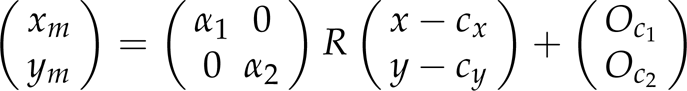
where α1 and α2 are positive constants, which are dependent on the depth information, focal length, scalar factors along u axis, and v axis, respectively; and
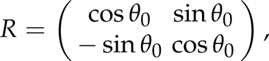
where θ0 denotes the angle between X axis and y axis with a positive anticlockwise orientation.

Nonholonomic wheeled mobile robot under a fixed camera
From (1), (2) and (3), by using a simple derivation, the image-based kinematical equation of the robot can be obtained:
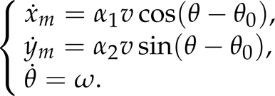
In the field of visual servoing control of robots, usually the camera parameters α1, α2 and the angle θ0 can be gotten by calibration. But this process will take a lot of time, which implies that it is impossible to use this method in high requirement of real-time. Therefore, it is necessary to consider how to design a control law in the case of dealing with these uncalibrated parameters.
As in [25], we make the following assumption:
Assumption 1: θ0 = 0, α1, α2 are unknown and bounded, the bounds of which are known positive constants:

Remark 1: Compared with it in [25], our assumptions are more relaxed since it is not necessary to suppose α1 = α2 in this paper.
Under this case, system (4) can be rewritten as

taking a state and input transformation [41]:

we obtain

It is noted that system (5) is so-called canonical chained-form with three-order and two control inputs u0, u1. The finite-time stabilization problem of (5) can be completely addressed by applying the controller given in [35], moreover, the authors have dealt with the nonholonomic chained systems with uncertain parameters and a matched disturbance.
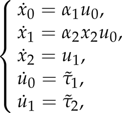
In this paper, we will consider the finite-time stabilization problem of the extended chained-form systems (6) with unknown parameters α1, α2, uncertain control direction γi(t), (i = 1,2) and unmatched un-modeled dynamics (or external disturbance) ϕ i (t), (i = 1,2).

where τ1 and τ2 are the new control inputs, the bounded measurable functions γ i (t), ϕ i (t), (i = 1,2) are supposed to satisfy that

here
Remark 2: Usually, the new control inputs τ1 and τ2 in the extended nonholonomic system (6) can be seen as the form of force or torque inputs, which is more practical than the form of velocity or acceleration controller u0 and u1 of (5) in the engineering application, because the new controller can be easier to implement for electrical engineer.
The following lemmas and conclusions are needed for our controller design later.
Lemma 1 ([42]): Considering the following system

suppose there exists a continuous function
There exist real numbers
Then the origin is a finite-time stable equilibrium of system (7). If U = U0 = R n , then the origin is a globally finite-time stable equilibrium of system (7).
Lemma 2 ([43]): If

Lemma 3 ([44]): For x ∊ R,y ∊ R, let c,d be positive real numbers, then

Lemma 4 ([43]): For x i ∊ R, i = 1,2,…, n, 0 p ≤ 1 is a real number, then the following inequality holds:

Theorem 1: Consider an uncertain nonlinear system:
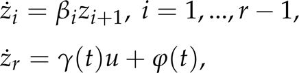
where z ∊ R r is the state vector and u ∊ R is the control input. Unknown parameters β i > 0, (i = 1,2,…, r – 1), the functions ϕ(·) and γ(·) are arbitrary measurable functions that represent bounded uncertainty:

where

if there exist a state-feedback control law ū0(z), a positive definite C1 function
Let

then system (11) is finite-time stable with respect to the origin.
Proof.: See Appendix A. □ Next, the control task is to present a switching controller for system (6) such that all the states converge to the origin equilibrium point in a finite time.
In this section, the main results will be presented. Firstly, we will state the basic idea to design a switching controller for system (6).
Motivated by the results of Theorem 1, we give a finite-time stable controller for the following system:
where

and the other is
Based on which, by using the design method of Theorem 1, we will propose a switching controller such that all the states of system (6) can be stabilized to zero in a finite time.
According to the design idea above, a discontinuous switching controller is presented as follows.
Let

where

where Λ 0, q0 ∊ (0,1) are design parameters. Then there exists a finite time T1 +∞ such that <u0(t) = 1 as t ≥ T1, and go to Step 2.
Let

where

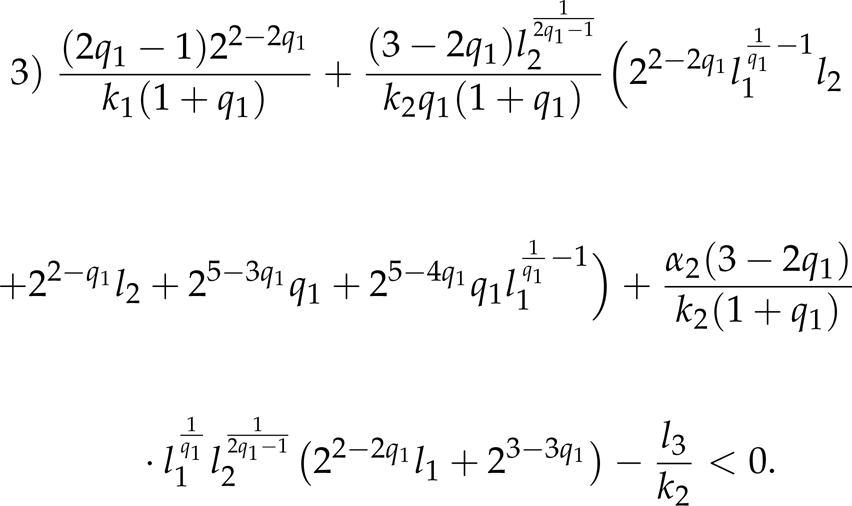
q1 = p/q ∊ (2/3, 1), p, q are positive odd integers, l i > 0, (i = 1,2,3) k j > 0, (j = 1,2) are design parameters satisfying the following conditions:


Then there exists a finite time
Step 3: Let

where

q2 = p1/q1 ∊ (0,1), p1, q1 are positive integers,


Then there exists a finite time
Theorem 2: Under Assumption 1, the switching controller composed by Step 1 ~ Step 3 in Section A ensures that system (6) can be stabilized to zero in a finite time.
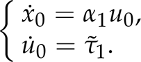
Proof. Firstly, in Step 1, for a first-order system

Choosing a lyapunov function

which can be rewritten by

Hence, according to Lemma 1, it's clear that under the controller

because

and

By (20), (22)-(23) and from Theorem 1, system (21) can be stabilized to zero in the finite time T1 with the controller τ1, i.e., u0(t) =1 as t ≥ T1.
Next, in Step 2, substituting u0 = 1 into the subsystem (13), it has

Take a positive definite, radially unbounded function about x1

Its time derivative along (24) is

where

As in [44], we take a C1, positive definite and proper Lyapunov function about (x1, x2) as follows

We can obtain
where
Then

where
By using (8) in Lemma 2, we have

Note that

From (27)-(28) and (9) in Lemma 3, we have

Substituting (25), (27) and the formula above into (26), we have

Because

Applying Lemma 3 again, we have

Taking a Lyapunov function about (x1, x2, u1) for system (24) as follows

Let

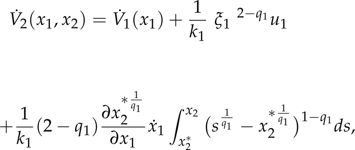
and the time derivative along (24) is

Note that

Thus

From (8) in Lemma 2, it has

From (28), (31) and (10) in Lemma 4, it has

Therefore, from (32), we have

By using (33) and Lemmas 2–4, we have

Substituting (29), (32)-(34) into (30), we have

Because

and

substituting (36) and (37) into (35) has

From (15)-(17), we can rewrite the formula above as follows

where


According to the definition of V3(x1,x2,u1), by using (27) and (31), we have

Let

it has


then we can obtain

Formulas (42)-(43) ensure that controller (37) can stabilize system (24) to zero in a finite time. Furthermore,

Therefore, according to Theorem 1, subsystem of (6)

can be stabilized to zero in a finite time T2 by the controller τ2 in Step 2.
Finally, by using the similar proof method, it's simple to prove that the subsystem of (6)

can be stabilized to zero in a finite time T3 by the controller τ1 in Step 3. For brevity, here omit the detailed process in this step. And this completes the proof of Theorem 2. □
Remark 3: Note that, if we choose sufficiently large k1 and k2 in (15)-(17), then it's possible to find a group of feasible solutions for the design parameters although it's difficult to obtain all the solutions of these parameters as pointed out in [46]. Here, we propose a simple search algorithm for finding a group of feasible solutions of the parameters step by step as follows:
First, choose
Step a: Given a sufficiently large


Select k2 > 0 satisfying (47)-(49):


If

Step b: Select l1, l2, l3 such that

Remark 4: As for (18)-(19), we can choose

Finally, we select
Remark 5: In this paper, we present a finite-time switching controller for the uncertain robot systems, but it is challenging to estimate the bounds for the settled time, because this time depends on the bounds of uncertain parameters, the external disturbance and the initial state value.
In this section, the switching controller proposed in Theorem 2 is used to show how to stabilize the uncertain visual feedback system (6) in a finite time. We will demonstrate the effectiveness of our methods by an example.
In the following simulation, we assume that:
Figures 3–5 show some simulation results with MATLAB. Figure 3 shows that the state variable (x0, u0) goes to zero in a finite time t ≤ 35s. From which, one can observe that u0 is stabilized to a constant (u0 = 1) and keep it in Step 2 until it is driven to zero together with x0 in the last step.
Note that in Figure 3, for u0, during the control process, we design a controller τ1 to make it converge to the constant 1 in Step 1 - Step 2, while in Step 3, we give another robust controller τ1 such that (x0, u0) can be stabilized to zero in a finite time, and thus, we find that there is a peak at t=25s because of using this discontinuous switching controller.
Figure 4 shows the state (x1, x2, u1) can be stabilized to zero step by step within the finite-time interval [0, 35s] under this switching controller (τ1, τ2) demonstrated in Figure 5.

The response of the state variable (x0, u0) with respect to time

The response of state variable (x1, x2, u1) with respect to time
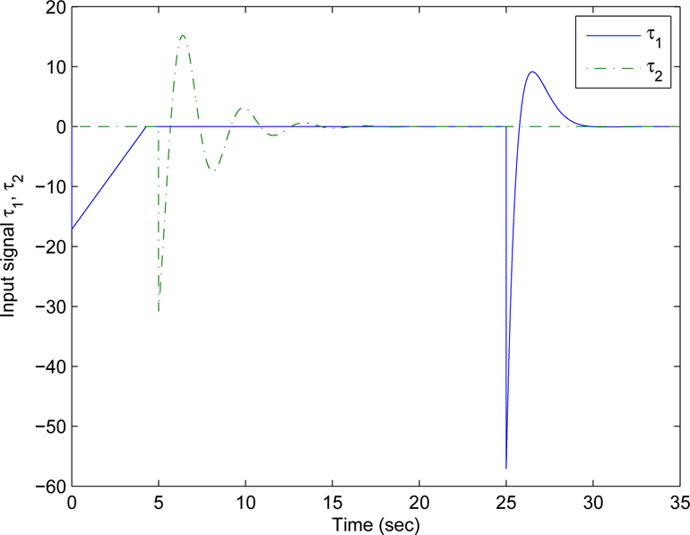
The response of the control input (τ1, τ2) with respect to time

The response of the state variable x m with respect to time

The response of the state variable y m with respect to time

The response of the state variable θ with respect to time
Additionally, the following simulation results Figures 6–8 are about the original mobile robot system with visual servoing (4), from which, we can observe that the system state (x m , y m , θ) can also be stabilized to zero in a finite time.
In this article, a new switching controller is presented for solving the global finite-time stabilization problem of the nonholonomic mobile robots based on visual serving with uncalibrated camera parameters and external perturbation. The best innovation of this paper is that the discontinuous controller design is based on applying the stability theorem of finite-time and a new switching design method such that the states of closed-loop system can be stabilized to origin point in a finite time. In the near future, we will discuss the corresponding finite-time stabilization problem with saturated control inputs.
Footnotes
6.
This paper was supported by the National Science Foundation of China (61304004, 61203014, 11274092,1077403), the China Postdoctoral Science Foundation funded project (2013M531263), the Jiangsu Planned Projects for Postdoctoral Research Funds (1302140C), the National Science Foundation of Jiangsu Province (BK2012283), the Ministry of Education of Jiangsu Province (1066-B11025), the R & D Special Fund for Public Welfare Industry (201101014), the Ministry of Education of China (MS2010HHDX044) and the National Basic Research Program of China (973 Program) (2010CB832702).
Appendix A.
Adopt the similar proof method as it in [45], the time derivative of the Lyapunov function
Because
On the other hand, if
Therefore, we have
According to Lemma 1, any a non-trivial trajectory z of system (11) reaches zero and stays there in a finite time.