Volumetric Next-best-view Planning for 3D Object Reconstruction with Positioning Error

Abstract

Three-dimensional (3D) object reconstruction is the process of building a 3D model of a real object. This task is performed by taking several scans of an object from different locations (views). Due to the limited field of view of the sensor and the object's self-occlusions, it is a difficult problem to solve. In addition, sensor positioning by robots is not perfect, making the actual view different from the expected one. We propose a next best view (NBV) algorithm that determines each view to reconstruct an arbitrary object. Furthermore, we propose a method to deal with the uncertainty in sensor positioning. The algorithm fulfills all the constraints of a reconstruction process, such as new information, positioning constraints, sensing constraints and registration constraints. Moreover, it improves the scan's quality and reduces the navigation distance. The algorithm is based on a search-based paradigm where a set of candidate views is generated and then each candidate view is evaluated to determine which one is the best. To deal with positioning uncertainty, we propose a second stage which re-evaluates the views according to their neighbours, such that the best view is that which is within a region of the good views. The results of simulation and comparisons with previous approaches are presented.

1. Introduction

Three-dimensional (3D) models of real objects are used in several robotic applications, such as object manipulation, pose estimation and tracking. There are at least two ways to obtain a 3D model of an object. The first is by CAD modelling; unfortunately, this way requires a skilled human modeller. The second way is by object reconstruction, which consists of taking several scans of the object's surface with a range sensor (see Fig. 1). The sensors or scanners must be placed in different locations because they have a limited field of view and also because the objects have self-occlusions. The set of different locations (or views) must be chosen carefully, such that each location satisfies certain acquisition constraints (in the next section, we discuss these constraints). A human operator can select these views, as in the Michelangelo Project [1]; however, human intervention should be reduced as much as possible in robotics applications. Another way to get these views is to place the sensor in a predefined set of views around the object [2], but this solution cannot be adequate given different object shapes and sizes. Thus, the best solution for robotics applications is a view planning algorithm which can automatically find each sensor location [3].

Figure 1.

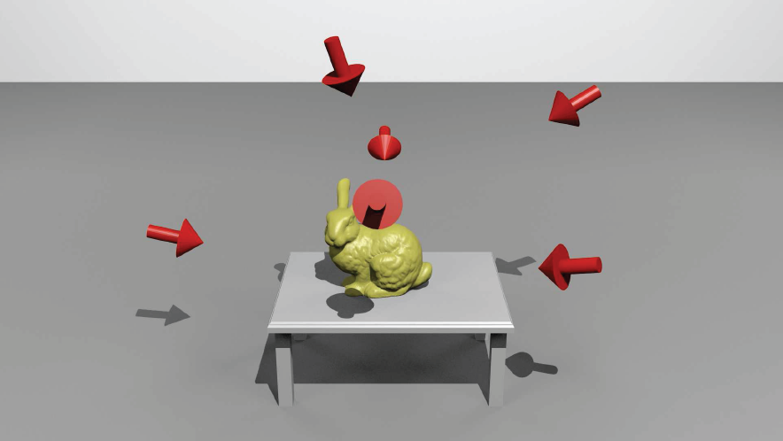
Required views to build a 3D model of an object. The arrows indicate the position and orientation of the sensor, from which a scan is taken.

1.1 The Next Best View Problem

Planning all the required views in advance is not possible because the object is unknown; instead, view planning must be done concurrently with the reconstruction process in a sequence of steps involving robot positioning, scanning, registration and planning of the next view. Fig. 2 shows the task flowchart.

The problem addressed in this paper is to plan the next sensor's position, called the ‘next best view'(NBV). The NBV is the best view for the reconstruction process from a set of candidate views. Determining the NBV is a complex problem because the determined view must fulfil the following constraints:

1. New information. The NBV must see unknown surfaces in order to completely observe the object.

2. Positioning constraint. The view must be reachable by the robot and there must be enough space around the view location for the robot's placement.

3. Sensing constraint. The surfaces to be seen must be within the camera's field of view and depth of view; in addition, the angle formed between the sensor's orientation and the surface normal must be smaller than a given angle defined by the sensor in question [4].

4. Registration constraint. To ensure that the new scan will be merged with the previous ones, there must be an overlap between them. This overlap is used by algorithms like iterative closest point [5] to merge the surfaces. In some cases, this overlap is also used to update the camera's pose and decrease the positioning estimation error.

Figure 2.

Object reconstruction process. One iteration of the process consists of four steps: positioning, scanning, registration and planning.

Figure 3.

Output model from our view planner for a bunny object. All the sub-figures show the voxel representation. Sub-figure a) also shows the voxel normals.

In addition to the previous constraints, there are certain other desirable characteristics that the NBV should have. These desirable aspects are not completely necessary, but they can improve both the reconstruction process's efficiency and the 3D model:

• Greatest unknown area. A given view should see as much of the unknown surface as is possible so as to reduce the number of required views. This characteristic increases in importance if the number of scans is limited.

• Navigation distance. Given that travelling from the current sensor position to the NBV consumes time and energy, it is desirable that the navigation distance should be short.

• Perpendicularity. If the angle formed between the surface normal and the sensor's orientation is close to 0, the scan surface will have better quality. This desirable characteristic is named scan's quality [6].

• Spatial uncertainty. Robots implement non-ideal positioning. The consequences of such error are: (i) decreased coverage, (ii) different precision and density than expected, and (iii) reduced visibility of the surface [7]. Therefore, the planned view should decrease these consequences.

1.2 Contributions

We present a NBV algorithm that can reconstruct arbitrary 3D objects. Fig. 3 shows a 3D model of an object obtained with our method. The algorithm follows a search-based paradigm, where a set of candidate views is computed and then every view is tested to determine whether it is the best view. In this paradigm, a utility function is used to evaluate how good a view is.

The first contribution is a utility function that evaluates most of the constraints (the constraints that are not evaluated by the function are fulfilled during the generation of the candidate views). We consider our function to be more comprehensive than previous functions. For example, this function is one of the first to use the navigation distance as an important factor to determine the NBV; additionally, it is directly applicable to certain types of robots, like quadcopters and coordinate measurement machines. The second contribution is an efficient search strategy. This strategy reduces the time to evaluate the candidate views. The third contribution is a method for re-evaluating the candidate views in order to decrease the positioning error effects.

2. Related Work

Researchers have addressed the NBV problem since the 1980s. Previous works can be divided according to two types: search-based methods and occlusion-based methods. Search-based methods use an optimization criteria to find the NBV among a set of candidate views. Occlusion-based methods use the occlusion boundaries within the range image of the current view to determine the NBV. Our algorithm is a search-based method, and as such we will mainly review similar methods in this section. For an extended review of all the methods, see [3].

The early works [8], [9] and [10] aimed to find the view that provides the ‘greatest unknown area’ (GUA). Banta and others in [9] used a combination of occlusion-based and search-based algorithms. They proposed to use the occlusion edges (called ‘jump edges') of the range images to generate some candidate views, after which they constructed a ray tracing in order to determine which candidate view will disclose the most hidden point information. Wong, in [10], proposed an ‘optimal method’ where a set of views around the object is created and each view is evaluated; unfortunately, the method requires significant computation time.

The view that provides the ‘greatest unknown area’ (GUA, for short) from the early works is sometimes not the best choice because other constraints need to be satisfied. To address this limitation, other methods have been proposed. Massios, in [6], included a quality factor in the utility function. Sanchiz, in [11], proposed a utility function including overlap and unknown areas.

Other works have included essential constraints in view planning and have proposed techniques to compute the NBV within a short time. In [12], Blaer and Allen proposed a method that determines the NBV from a set of candidate views - they reduced the computation time by means of looking for just one type of voxel (called a ‘boundary voxel'). However, the view planning phase only looked for the greatest unknown area, leaving certain constraints like overlap and navigation distance. In [13], Low and Lastra proposed a way to join views and voxels into patches - based on this, they proposed a hierarchical strategy to find the NBV within a short time. However, their utility function does not consider the navigation distance or scan quality. Foissotte et al. in [14] proposed a new way to find the GUA using an optimization technique; however, they do not specify how to solve for the object's self-occlusions.

New methods include motion planning for fixed arms in order to reach the planned views. In [15], Kriegel et al. combined two approaches for determining the NBV - a surface-based method and a volumetric method. First, they computed a set of candidate paths over the triangular mesh border; then, they evaluated the goodness on the volumetric representation. The goodness was evaluated with information gain (IG), while in the present work the goodness is determined by the combination of several desired characteristics. Another work is that of Torabi and Gupta [16]. In their work, the authors plan a NBV from a set of candidates in the workspace and then use inverse kinematics to obtain a configuration that matches the desired sensor location in the workspace. The novelty of the method is in the generation of the candidates and the stop criteria. The candidates are synthesized over the borders of the scanned surface and the stop criteria ensure that if the surface has no more candidates then the model is completed. Krainin et al. [17] proposed a method in which the robot grasps the object and moves it inside the camera's field of view (FOV); the candidate views are evaluated with a trade-off between the view goodness and the motion cost. One limitation of the approach in [17] is that the robot might not have the ability to grasp and move the object. In [18], the authors address the problem of actively searching for an object in a 3D environment with a humanoid robot. The authors have proposed a ‘greedy’ strategy for selecting the next best view and they have shown that fast and reliable 3D object localization is feasible (if certain reasonable constraints on the problem are fulfilled). These constraints include placing bounds on the size of the search space, having controlled illumination conditions, and small dead-reckoning errors. However, the work in [18] does not address the problem of the reconstruction of the sought model.

The previous work has focused on reconstructing an object with high coverage. However, such works have not been tested in scenarios where the positioning system has low accuracy, such as with quadcopters and mobile robots. Scott [7] notes that the pose error can cause serious scanning deficiencies. In this paper, we propose a NBV method that predicts the error and plans a view to compensate for it.

The work we report here represents a combination and an extension of our previous work. In [19], we have proposed a utility function that provides a complete evaluation of the views - it includes unmarked surfaces, quality, overlap and distance. In [20], we presented a method for dealing with position error in the context of NBV planning. In this paper, we combine these two methods in a coherent manner, describing in more detail the proposed approaches, and we perform additional experiments comparing the method with the related work.

3. Method Overview

Our method is based on the dual assumption that the robot knows the position and the approximated dimensions of the object in question. The method is summarized in algorithm 1 and is explained now. In the first step, the robot performs a scan with the range sensor. If there are scans taken from previous iterations, they will need to be registered and merged to build a unique model. Such registration is concerned with matching point clouds into one reference frame. This task is carried out by an ICP [5] algorithm, which iteratively minimizes the distances between the overlap of two sets of 3D points. After registration, the redundancy between the overlapped areas is decreased and a surface representation is created; in this work, we use a voxel map representation, which is explained in section 4. Afterwards, the robot computes a set of candidate views around the object. Next, all those candidate views that do not fulfil the positioning constraints are deleted, leaving only a set of feasible views.

Algorithm 1:

3D object reconstruction with view planning

The set of feasible views is evaluated using a utility function (during the evaluation, we perform a ray tracing whereby the sensing constraints are considered). Next, a re-evaluation of the views is performed in order to select views robust to any positioning error. Next, the views are ranked and the best evaluated view is selected as the NBV. This process allows us to evaluate and satisfy all the constraints.

Once the NBV has been chosen, the robot moves the sensor to the NBV position. If something comes up and the robot cannot reach the position, a new NBV is computed. Otherwise, when the robot reaches the position, the scan is performed and the information is registered with the ICP algorithm. Afterwards, the partial model is updated.

At this point, the model may be complete or not. However, since we do not know the real object, we cannot know if the model is complete. As such, a new view is computed. If the new computed view provides new information, the process is repeated until the NBV does not provide new information.

We use a voxel map to store the information about the reconstruction scene. A voxel is the smallest volume of an object and a voxel map is a 3D vector where each unit is a voxel. Using a voxel map has certain advantages: (i) a voxel can represent many surface points that are inside its boundaries, speeding-up the NBV computation and the model display, and (ii) a voxel map is easily implemented because it is only a 3D vector.

4. Scene Representation

Each voxel has three associated attributes: (i) a label, (ii) a normal value, and (iii) a quality value [11]. The label of a voxel indicates its type according to the different areas that exist in a given reconstruction scene (see Figure 4):

Figure 4.

Horizontal slice from a reconstruction scene. The figure shows the different types of areas that appear when a scan is taken.

• Unmarked voxel. This is a voxel that has not been seen by the sensor. When the algorithm starts, a cube of ‘unmarked’ voxels is placed in the space where the object is.

• Occupied voxel. This voxel represents a surface scanned by the sensor. After a scan has been taken, all the voxels whose positions correspond with measured points are labelled as ‘occupied’ voxels.

• Empty voxel. These voxels represent empty space. After a scan, all the unmarked voxels between a measured point and the sensor position are labelled as ‘empty’ voxels.

• Occluded voxel. These voxels represent an area that was within the sensor's field of view but which was occluded by a surface. All the unmarked voxels that have been occluded by occupied voxels are labelled as ‘occluded’ voxels.

• Occplane voxel. An occplane is a contraction of ‘occlusion plane'. This type of voxel is part of the occluded space, but it is on the boundary of this space. Formally, it is an occluded voxel that is adjacent to an empty voxel.

Normal and quality attributes are only defined for occupied voxels. The normal attribute is related to the surface normal and the quality attribute is related to the perpendicularity of the sensor with respect to the surface. To obtain the attribute normal, we first determine the surface normal of every point within the range image; next the average of the surface normals from the points whose positions coincide with the voxel position is obtained; finally, the normal attribute is equal to the average obtained. In addition, to obtain the quality attribute, we first determine the sensed quality of each point of the range image as the cosine of the angle formed by the point's surface normal and the sensor's orientation. The greatest sensed quality from the points that match up with the voxel position is the quality attribute.

The process followed in order to update the voxel map is based on the Sanchiz algorithm [11], whereby the positions of the sensor and the points of the scanned surface are used to update it.

4.1 Candidate Views

The set of candidate views, V, is evaluated to determine the NBV. When there is no positioning error, we use a set of candidate views around the object - this configuration is often called a ‘view sphere;, where each view is equidistant from the centre. To generate the view sphere, we use a technique called ‘sphere tessellation'. This technique starts from an icosahedron and tessellates each face to create four new faces; the tessellation process is repeated recursively until the tessellation level required is achieved. Next, the centroid of each face is taken as a view position and it is oriented to the sphere's centre.

When there is a positioning error, the views are not restricted to a view sphere but are instead distributed inside a cube. The cube is divided as a 3D grid and the position of each cell is taken as a candidate view. Each candidate view is pointed towards the object (the centre of the cube). The cube is defined by three orthogonal line segments: S_x, S_y and S_z. The 3D grid is obtained by dividing each segment S_x, S_y and S_z in n cells, generating a set of n³ views.

4.2 Candidate View Evaluation

The evaluation of each view in V is done in two steps: ray tracing and utility function evaluation.

The ray tracing consists of tracing a set of rays inside the voxel map according to the Bresenham algorithm [21]. The ray tracing is configured according to the sensor parameter—field of view, the resolution (rows × columns), the sensor view angle and the depth of view —. When a ray ‘touches’ a voxel (as distinct from empty voxels), the attributes from this voxel are stored. After ray tracing, we have all the information about the voxels that are ‘visible’ from the candidate view. In other words, we have the number of occupied voxels (n_oc), the number of occplane voxels (n_op), the number of unmarked voxels (n_um), and the quality and the normal for each occupied voxel. We call number of rays of the ray tracing the ‘ray tracing resolution’ (RTR). A full RTR is equal to the resolution of the sensor used to scan the object.

In the second step, the information obtained from the ray tracing is used by the utility function to get a numerical value for each candidate view.

5. Utility Function

The utility function quantifies the desirability of a view based on the NBV constraints given in section 1.1. This utility function is formed by several factors that quantify each constraint of a desirable view. Each factor is detailed below and, at the end of this section, the complete function is presented.

5.1 Area Factor

The objective of the area factor is to perceive unseen areas and to provide, at the same time, some overlap with previous scans. This objective is achieved when the NBV provides a certain percentage of each voxel-type. For instance, a view that sees only occupied voxels is a bad view because it does not have unknown areas; a view that sees only occplane voxels is also bad because it does not provide overlap. As such, the best view is that which sees a percentage of occupied and occplane voxels. Accordingly, the area factor evaluates the percentage of each voxel1 looking for a desired percentage2.

Mathematically, the area factor is represented by a sum of functions,

$$\begin{array}{l}{f}_{area}={\displaystyle \sum _{i=1}^2}{f}_i\hfill \end{array}$$

(1)

where each f_i evaluates the percentage of a certain voxel-type (occupied or occplane). Each function f_i gives a value within the range [0, 1] based on the voxel percentage seen by the ray tracing and the desired percentage for a given voxel-type. f_i reaches a maximum when the percentage x_i of voxels i is equal to the desired percentage, α _i ; this means that f_i = 1 when x_i = α _i . The function reaches a minimum when the percentage x_i is either 0 or 1 - that is to say, the candidate view does not perceive this type of voxel or else it only perceives voxels of this type. Figure 5 shows the desirable behaviour for each function f_i.

Figure 5.

The graph shows the desired behaviour for each function f_i. The x axis indicates the percentage of voxels of type i after ray tracing. α indicates the desired percentage for the voxel-type i; α can be between 0 and 1.

Next, we formally list in (2) the set of constraints for each function f_i (simplified to f), which in addition to the mentioned restrictions incorporates some smoothness and continuous restrictions:

$$\begin{array}{ll}f\left(0\right)=0\hfill & f^{\prime }\left(0\right)=0\hfill \\ f\left(\alpha \right)=1\hfill & f^{\prime }\left(\alpha \right)=0\hfill \\ f\left(1\right)=0\hfill & f^{\prime }\left(1\right)=0\hfill \\ f\left(x\right)>\mathrm{0,}\hfill & \forall x\in \left(\mathrm{0,1}\right)\hfill \\ f^{\prime }(x)>\mathrm{0,}\hfill & \forall x\in \left(\mathrm{0,}\alpha \right)\hfill \\ f^{\prime }\left(x\right)<\mathrm{0,}\hfill & \forall x\in \left(\alpha \mathrm{,1}\right)\hfill \\ \hfill & \hfill \end{array}$$

(2)

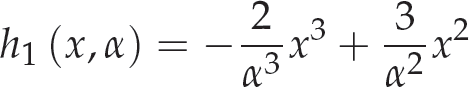
To model the behaviour required by the constraints: (i) we first propose the use of a polynomial as a template function, and (ii) we then find the coefficients of the polynomial, so that the constraints are satisfied. In this case, we use a third-degree polynomial divided into two parts as our template function (a lower-degree polynomial gives negative values):

$$f=\{\begin{array}{cc}{A}_1{x}^3+B_1{x}^2+C_{1}x+D_1\mathrm{,}& 0<x\le \alpha \\ A_2{x}^3+B_2{x}^2+C_{2}x+D_2\mathrm{,}& \alpha <x<1\end{array}$$

(3)

Substituting the constraints (2) in function (3) and its derivative, we get a system of four equations and four variables (the coefficients) for each polynomial. Solving the systems, we find the coefficients. Next, substituting the coefficients in (3) leads to equation (4), formed by expressions (5) and (6). It is worth noting that equation (4) depends only on α and x - this makes it possible to adjust the desired percentage (α) for each voxel-type:

$$f\left(x\mathrm{,}\alpha \right)=\{\begin{array}{cc}{h}_1\left(x\mathrm{,}\alpha \right)\mathrm{,}& x\le \alpha \\ h_2\left(x\mathrm{,}\alpha \right)\mathrm{,}& x>\alpha \end{array}$$

(4)

where:

$$h_1\left(x\mathrm{,}\alpha \right)=-\frac{2}{{\alpha }^3}{x}^3+\frac{3}{{\alpha }^2}{x}^2$$

(5)

and:

$$\begin{array}{r}{h}_2\left(x\mathrm{,}\alpha \right)=-\frac{2}{{\left(\alpha -1\right)}^3}{x}^3+\frac{3\left(\alpha +1\right)}{{\left(\alpha -1\right)}^3}{x}^2\\ -\frac{6\alpha }{{\left(\alpha -1\right)}^3}x+\frac{3\alpha -1}{{\left(\alpha -1\right)}^3}\end{array}$$

(6)

Here, we have already defined f, which evaluates a voxel percentage depending upon the desired percentage. As such, the area factor is defined as follows:

$$f_{area}=f\left(x_{oc}\mathrm{,}{\alpha }_{oc}\right)+f\left(x_{op}\mathrm{,}{\alpha }_{op}\right)$$

(7)

where x_oc is the percentage of occupied voxels, α _oc is the desirable percentage for occupied voxels, x_op is the percentage of occplane voxels, and α _op is the desired percentage for occplane voxels.

In our implementation, we set α _oc = 0.2 and α _op = 0.8.

5.2 Navigation Factor

The objective of the navigation factor is to reduce the navigation distance between the current sensor position and the next view. This factor evaluates as the best view the one that is the closest to the current sensor position. Assuming that a sensor mounted on a robotic arm will move within a spherical surface around the object, the orthodromic distance - defined as the shortest distance between two points on a sphere - is a reasonable option. Therefore, in this work, we use the orthodromic distance. The minimum distance corresponds to the case in which the sensor does not move - it only changes its orientation. A maximum distance is determined by two opposite points on the sphere, and so we can define a normalized orthodromic distance x.

The behaviour of the navigation factor (Figure 6) must satisfy the following constraints: (i) the candidate view with the shortest distance must have the maximum value; (ii) the candidate view with the largest distance must have a minimum value given by ρ; (iii) a candidate view with a larger distance than other must have a smaller value; and (iv) at short distances, the value of the function must decrease more slowly than at large distances. Therefore, the constraints for the function are:

Figure 6.

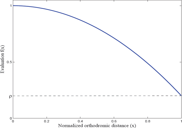
The graph shows the desired behaviour for the navigation factor

$$\begin{array}{ll}\hfill & f\left(0\right)=1f^{\prime }(0)=0\hfill \\ \hfill & f\left(1\right)=\rho \mathrm{,}0\le \rho <1\hfill \\ \hfill & f^{\prime }\left(x\right)<\mathrm{0,}\forall x\in \left(\mathrm{0,1}\right)\hfill \\ \hfill & \hfill \end{array}$$

(8)

We use a second-degree polynomial to model the desired behaviour:

$$\begin{array}{c}f\left(x\right)=A{x}^2+Bx+C\\ f^{\prime }\left(x\right)=2Ax+B\end{array}$$

(9)

Similar to the area factor, we substitute the constraints (8) in the polynomial (9). Next, we solve the system of equations. Finally, we find the expression of the navigation factor (10) in the function of x and ρ as follows:

$$f_{navigation}=\left(\rho -1\right)x^2+1$$

(10)

where x is the normalized orthodromic distance and ρ is the smallest value for the function.

5.3 Quality Factor

According to [6], a good scan is produced when the sensor is orthogonal to the surface; thus, the quality factor aims to place the sensor perpendicular to the surface. To achieve this, we use the already scanned area (the occupied voxels) to make a prediction regarding the new surface. Thus, the best view has an orientation which is orthogonal to the scanned area. Therefore, the quality factor is defined by equation (11), as previously used by Lozano in [22]:

$$f_{quality}=\frac{{\displaystyle {\sum }_{i=1}^{n_{oc}}\cos ({\alpha }_i)}}{n_{oc}}$$

(11)

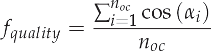
where α _i is the angle formed between the sensor's orientation and the surface normal of the occupied voxel i, and n_oc is the number of occupied voxels detected by ray tracing.

5.4 Occlusion Factor

The occlusion factor aims to determine occluded areas quickly (e.g., an object's self-occlusions). This factor gives a higher value to the view that sees more occplane voxels per ray tracing. Given this, the maximum number of seen occplane voxels might be the number of traced rays - we propose as the factor the ratio of occplane voxels per ray tracing:

$$f_{occlusion}=\frac{n_{op}}{rows\times cols}$$

(12)

where n_op is the number of occplane voxels, and rows and cols are the number of rows and columns of the range image generated by the ray tracing.

5.5 Utility Function

The complete utility function is a combination of the above factors. This combination considers as a primary factor the area factor and the others as secondary factors (the reason for this is that the main objective of the view planning is to reconstruct, as much as possible, the object, while an overlap is provided in each view):

$$f_{utility}=f_{area}*\left(f_{quality}+f_{navigation}+f_{occlusion}\right)$$

(13)

6. Search Strategy

An exhaustive search of the NBV tests each candidate view in V with the full RTR. As such, a densely approximated view sphere and a high RTR guarantees that a good view will be found. However, the computational cost is extremely high. In addition, the NBV algorithm will be implemented in a real robot and must operate in real-time. Therefore, a more efficient alternative is required. We propose a multi-resolution strategy to find the NBV quickly.

6.1 Multi-resolution Strategy

The multi-resolution strategy is based on the variability of the RTR while the number of candidate views and the voxel map remain unchanged. Algorithm 2 resumes the search strategy. This strategy consists of k stages. In each stage, a set of views is evaluated with a RTR for that stage. In the first stage, V is evaluated with a minimal RTR (R_min) (set by the user). The best evaluated views are selected for the next stage. In the next stage, the selected views are evaluated with a higher resolution. Again, the best evaluated views are selected. The process continues until the kth stage is reached whereby a reduced subset of views is evaluated with the ideal RTR (R_ideal):

6.1.1 Ideal Ray Tracing Resolution

The ideal RTR is closely related to the voxel map resolution, and we define it as the lowest resolution required for the ray tracing to cover the voxels of the model. When we use a RTR larger than the ideal, there is information redundancy because the traced rays are too close to each other, ensuring that more than one ray touches the same voxel. With the ideal RTR, the traced rays are separated from each other by a distance equal to the dimension of a voxel (pretending that only one ray touches each voxel).

Algorithm 1:

Computing the NBV with a multi-resolution strategy

Let us consider a voxel map that has a voxel length of len, a sensor that has a horizontal aperture of α and vertical aperture of β, and a sensor positioned at a distance r from the centre of the voxel map; then, R_ideal is computed as follows:

$$cols=\frac{\alpha }{\arcsin \left(\frac{len}{r}\right)}\mathrm{,}rows=\frac{\beta }{\arcsin \left(\frac{len}{r}\right)}$$

(14)

where cols is the number of columns and rows is the number of rows.

6.1.2 Intermediate Resolutions

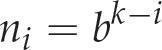
During the strategy, the RTR must be incremented for each stage. We propose a homogeneous increment between the minimal resolution (R_min) and the ideal resolution (R_ideal). As such, the RTR used for stage i is defined by equation (15):

$$R_i=R_{ideal}-(k-i)\times \left(\frac{R_{ideal}-R_{min}}{k-1}\right)$$

(15)

6.1.3 Selected Views

The number of selected views must decrease when the stage is increased. We propose equation (16) to determine how many views should be selected for each stage:

$$n_i=b^{k-i}$$

(16)

where b is a parameter selected by the user.

6.1.4 Number of Stages

The number of stages depends upon the number of candidate views. If the number of candidate views increases, then the number of stages increases. This relationship is defined by equation (17):

$$k=argmax\left(b^k<\left|V\right|\right)$$

(17)

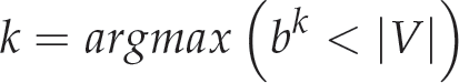
where |V| is the number of candidate views.

This makes the strategy independent from the number of candidate views and leaves the parameters R_min and b for the user.

7. Convolution After Evaluation

Usually, the planned view is not reached by the positioning system. For precise fixed arms, turntables or a Cartesian robots, the error is close to zero, but for low-cost platforms or mobile robots, the error is greater. Some consequences of the positioning error are the increment of the number of required views and the failure of the image registration - in consequence, the failure of the model reconstruction. Scott, in [7], provides a more detailed explanation about the consequences of this error in terms of how it affects: (i) the sensor coverage, (ii) the surface's visibility, and (iii) the precision and sampling density. We propose a method which deals with the positioning error. We alter the definition of the NBV thus: ‘the NBV is the view which is in the centre of a high evaluation region'. We define a region as the set of views which are close to a view according to its Euclidean distance in R³. With the mentioned idea, we want to ensure that although the sensor does not reach the planned position, it will fall into a ‘good’ position.

We propose to re-evaluate the views according to the value of their neighbours and the distribution of the error. To perform this task, it is necessary to increase the value of a view when the neighbours are ‘good’ and to reduce the value when the neighbours are ‘bad'. In addition, the re-evaluation should depend upon how likely it is to fall for one neighbour. One way to perform this task is to make a convolution between the utility function and an error function. The error function represents the distribution of the positioning error. The result is an average of the utility. Below, we detail the performed convolution.

Let x and τ be Cartesian coordinates in R³: x represents the view position and τ the error, f is a multi-dimensional Gaussian function representing the error distribution and g is the utility function. Then, the convolution is given by equation (18):

$$[f*g](x)={\displaystyle \int }f(\tau )g(x-\tau )d\tau$$

(18)

The function f is defined by a multidimensional Gaussian function according to equation (19):

$$f(\mu \mathrm{,}\Sigma \mathrm{,}X)=A\exp \left[-\frac{1}{2}{(X-\mu )}^T{\Sigma }^{-1}(X-\mu )\right]$$

(19)

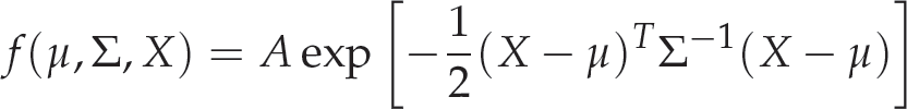
where X is the error random variable, μ is the mean error and Σ is the covariance matrix. For convenience, we have established the parameter A = 1 to keep the maximum value at one.

The NBV is now the view with the highest evaluation after the convolution. Figure 7 shows an example of how the search space is modified by the convolution. In the example, we can see how the NBV is moved to a safe place. With this method, although the planned view could not be reached, it is highly plausible that the sensor will end with a good view.

Figure 7.

Plot of the candidate view's utility before and after convolution Each graph shows the utility of a view. The axes x and y represent the coordinates of the view and axis z (up) represents the utility. The experiment places several views in concentric spheres around the object of interest (the object lies at coordinates (10, 10)), each view was evaluated and, later, the convolution was performed.

Equation (18) computes a continuous convolution. However, for the robotic application, we have implemented the method using the discrete convolution defined by equation (20):

$$(f*g)[v]={\displaystyle \sum _{i=1}^{n^3}}f[m_i]g[v-m_i]$$

(20)

where v belongs to the candidate views set and m_i belongs to M, a set of possible errors.

8. Experiments Without Positioning Error

Our algorithm was first tested in simulation without positioning error. In this part, we describe the three experiments. The first one shows the reconstruction of several objects. The second one shows how the navigation factor affects the reconstruction. Finally, the third one gives a comparison of our approach with previous approaches (Section 9 details the experiments with positioning error and the use of the convolution after evaluation).

8.1 Simulation Configuration

A time-of-flight camera was simulated and the objects were taken from virtual models. The simulated range camera has 45 degrees for the horizontal and vertical apertures and a resolution of 320 × 320 points. The system was implemented in the language C and OpenGL. The machine used for the tests was an AMD Turion64 with 2 GB RAM.

The objects used are shown in Figure 8(a). These objects have different shapes and exhibit incremental difficulty for the reconstruction process: the sphere is a convex simple object; the pear and the banana are non-convex; the mug, bunny and dragon are non-convex with self-occlusions; and, finally, the SGI logo has holes and self-occlusions.

Figure 8.

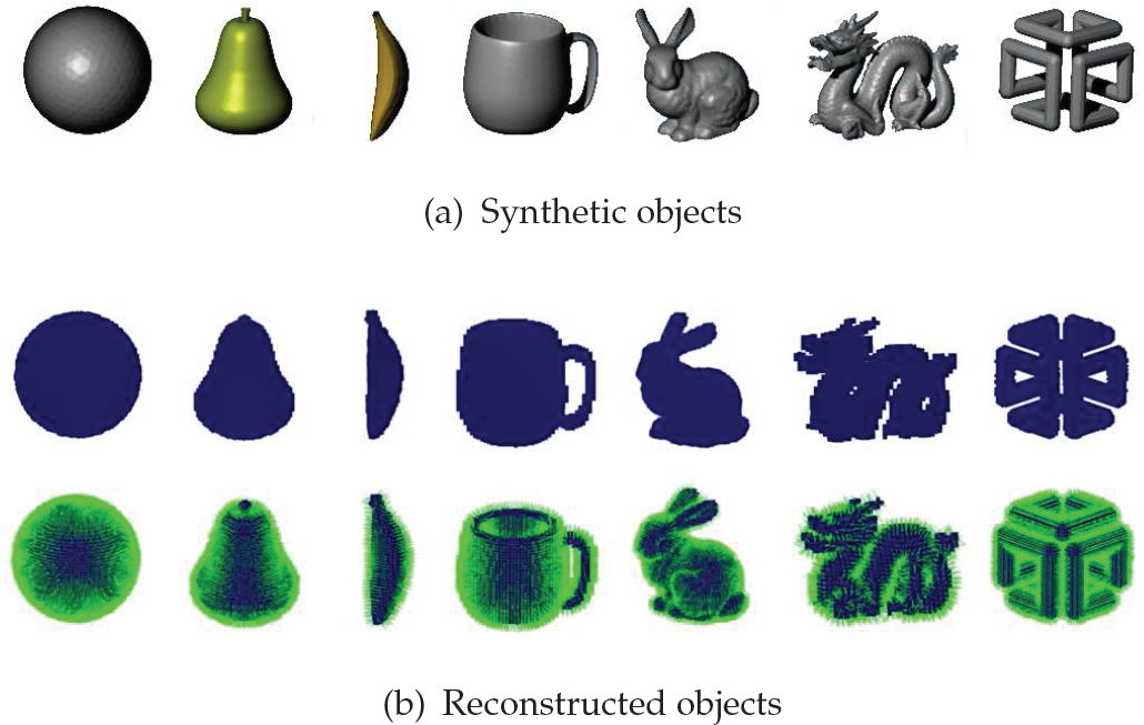
3D Objects. In the top row are the CAD object models used to perform the simulation, in the centre row are the voxel representations of the reconstructed objects, and in the bottom row are the voxel representations with surface normals.

8.2 Reconstruction

In this experiment, we reconstructed the seven different objects. The voxel map dimensions were 205 × 205 × 205 (8 615 125) voxels for the scene and 55 × 55 × 55 (166 375) voxels for the object enclosure. The voxel size was 0.02 m. We used a view sphere with a radius of 2 m and 80 candidate views. We used a multi-resolution strategy with the parameters k = 2, b = 10, R_min = 40×40.

Tables 1 and 2 show the results for the exhaustive and multi-resolution strategies, respectively. Column Views shows the number of views required to complete the model; Occup shows the amount of occupied voxels in the voxel map at the end of the reconstruction; Qual shows the voxel map quality (mean quality of all occupied voxels); and Dist shows the total travelled orthodromic distance measured in metres. Figure 8(b) shows the reconstructed models.

Table 1.

Reconstruction data for each object using the exhaustive strategy

Object	Views	Occup.	Qual.	Dist.(m)
Sphere	6	7200	0.757	17.70
Pear	7	4330	0.803	16.40
Banana	4	1050	0.803	9.54
Mug	8	7736	0.718	21.76
Bunny	9	5392	0.825	21.32
Dragon	9	3595	0.777	24.46
SGI logo	12	11952	0.843	34.02

Table 2.

Reconstruction data for each object using the multi-resolution strategy

Object	Views	Occup.	Qual.	Dist.(m)
Sphere	6	7200	0.757	17.70
Pear	7	4342	0.803	16.40
Banana	4	1049	0.765	7.15
Mug	8	7736	0.718	21.76
Bunny	9	5395	0.821	23.56
Dragon	9	3639	0.798	22.14
SGI logo	12	11900	0.832	32.53

These experiments show that the algorithm has the ability to reconstruct objects of different shapes. Besides this ability, it provides overlap in each scan and reduces the navigation distance. The number of required views is quite similar to those reported in [10], where a similar voxel resolution was used; however, in that work each view does not ensure overlap. In addition, the algorithm fulfills all the constraints of a NBV as described in the introduction.

8.2.1 Multi-resolution Strategy

The average time required to compute each NBV was 6.2 s using the multi-resolution strategy and 135.5 s using the exhaustive strategy. The multi-resolution strategy reduces the required time more than 20-fold while preserving its effectiveness (compare Table 1 with 2). Multi-resolution is faster, given that a large set of views is rapidly evaluated with a low resolution, and only a small set of views is selected for evaluation with a higher resolution. One limitation of the multi-resolution strategy is that, at the end of the reconstruction, there are very small areas of occluded voxels, e.g., one single voxel, and they cannot be seen by the first stage of ray tracing (minimum resolution). Therefore, a trade-off between speed and surface cover should be considered. In our experiments, we achieve a high percentage of coverage for the configured parameters.

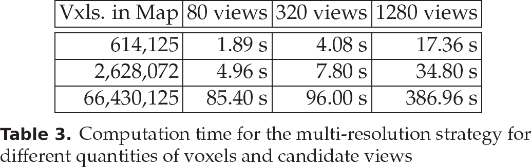
8.2.2 Voxel Map Resolution and Candidate Views

Our algorithm can work with different voxel resolutions and different numbers of candidate views. In Table 3, we show how the time increases when one increases the number of views and the number of voxels in the map. Our search strategy adapts to the configuration of the voxel map and candidate views. We can observe that the time required is proportional to the number of views and the voxel resolution. When we use the multi-resolution strategy, the saving in computation time is at least 20-fold compared to an exhaustive search. For instance, for 1,280 views and 2,628,012 voxels, the computation time of an exhaustive strategy is about 1,247 s; however, using the multi-resolution strategy the computation time is 34 s.

Table 3.

Computation time for the multi-resolution strategy for different quantities of voxels and candidate views

Vxls. in Map	80 views	320 views	1280 views
614,125	1.89 s	4.08 s	17.36 s
2,628,072	4.96 s	7.80 s	34.80 s
66,430,125	85.40 s	96.00 s	386.96 s

8.3 Navigation Factor Behaviour

In this experiment, we show the effect of the navigation factor in the reconstruction process. We ran the algorithm with and without the navigation factor in the utility function. Table 4 shows the results. We used the multi-resolution search strategy.

Table 4.

Comparison when the navigation factor is included (or not) in the utility function. The columns w show the results with the navigation factor and the columns wo show the results without it. In general, when the navigation factor is used, there is a reduction in the navigation distance. Furthermore, the distance reduction does not increase the number of required views.

Object	Views		Qual.		Dist. (m)
	w	wo	w	wo	w	wo
Sphere	6	6	0.75	0.75	17.7	20.9
Pear	7	7	0.80	0.82	16.4	19.7
Banana	4	4	0.76	0.81	7.15	9.50
Mug	8	8	0.71	0.72	21.7	22.7
Bunny	9	9	0.72	0.81	23.5	23.8
Dragon	9	9	0.79	0.78	22.1	28.4
SGI logo.	12	12	0.83	0.83	32.5	37.0

As we can see, there is a significant reduction in the distance travelled in five of the seven objects without increasing the number of required views. Namely, when the navigation factor is used, we can reconstruct the same percentage of the surface with a shorter travelled distance. This occurs because the algorithm prefers views that are closer to the sensor position. Usually, this factor reduces the navigation distance, but there are some cases where there is no reduction and the total distance is similar to that which does not use the factor; this happens because this algorithm is a greedy one and it is locally optimal (in each NBV) but it is not globally optimal (the set of views).

8.4 Comparison with Previous Approaches

In this paper, we use a combination of several factors (area, quality, distance, etc.) to determine the NBV, equation 13. In contrast, the previous works [6, 10, 12, 23] only look for the view that provides the greatest unknown area. In this experiment, we compare our ‘combination of factors’ (CF) approach with the ‘greatest unknown area’ (GUA) approach. We implemented the GUA approach with the utility function (21), which has a higher evaluation when the candidate view observes more occplane voxels.

$$f_{gua}=\frac{n_{op}}{rows\times cols}$$

(21)

where n_op is the number of occplane voxels, rows and cols are the number of rows and columns of the range image generated by the ray tracing.

Given that a reconstruction depends upon the initial view, we reconstructed each object several times from different initial views to make a fair comparison. We reconstructed the object mug (we consider it to be a difficult object due to its self-occlusions and holes) from 20 initial views; therefore, we have 20 reconstructions with the CF approach and 20 with the GUA approach. The results are shown in Figure 9 (the bars have been normalized). In the graph, we can see that, with the CF approach, the navigation distance decreased remarkably, the quality was improved and the number of occupied voxels (the surface seen) was quite similar, but the number of views increased slightly. This happened because, in our approach, we always have an overlap (we configured an overlap of 20%) so more views are needed to see the same area; however, the increase in the number of views is not too great (an average increase of 6%) compared with the overlap of 20%.

Figure 9.

Comparison with previous approaches. Our approach (CF) reduces the navigation distance, improves the quality and sees the same area (occupied voxels) as regards the GUA approach (see text for details).

In conclusion, our approach, generally reduces the navigation distance, improves the quality and sees the same area as compared with the GUA approach.

9. Experiments with Positioning Error

These experiments compare the performance of the convolution after evaluation (CAE) method in a scenario where there is positioning error. The performance is measured with the percentage of reconstructed surface per iteration. The error is simulated as a random variable with zero centred normal distribution. The comparison of the CAE method is made against the standard method (without convolution) in the same scenario with positioning error. We take the performance of the standard method as a baseline which has to be improved by the CAE method. In addition, we make a comparison with an ideal case, where there is no positioning error and the standard method is used. The ideal case will serve as a top-line performance. We expect that the CAE method can improve the baseline significantly and that it will be close to the top-line.

The objects reconstructed in this experiment are the sphere, the mug and the SGI logo (Figure 8) - they provide a sample of objects of different complexities. The reconstruction scene has been configured with the object in the centre and free space surrounding it. The positioning system is a free-flyer of five-DOF (x, y, z, pan, tilt). The utility function does not include the evaluation of the navigation distance, since the candidate views used in this part are not restricted to a sphere.

For these experiments, we have used the set of candidate views generated by the cube. We have divided the cube into 17 cells per dimension, given a total of 4,913 (17³) candidate views (|V| = 4913). For the purpose of speeding things up, we only considered views that were between an interior radius and an exterior radius - the evaluated views were 1,932. Our experiments considered only positioning error in the three axes (x,y,z) - we did not include positioning error in pan or tilt, which will be modelled in future work. Furthermore, we have assumed the following standard deviations: σ _x = 10 cm, σ _y = 10 cm, σ _z = 10 cm and conditional independence between the axes. We used a time-of-flight simulated sensor. It had a horizontal and vertical aperture of 92.5 degrees and 72.32 degrees, respectively, and it had an image resolution of 320 × 240.

The experiments consisted on running the planner three times per object: one with no error (σ₀ = 0 cm), the second with a positioning error with a standard deviation of 10 cm (σ₁ = 10 cm), and the third using the CAE method with the same error. First, we summarize the results for the sphere and the mug, and then we will present a more detailed discussion for the SGI logo reconstruction, given that it provides the most challenging object.

The reconstruction results for the sphere and the mug are summarized in Figure 10. The sphere's reconstruction achieves the same coverage with the three variants, given that it is a simple object and that there are no auto-occlusions. For the mug, the CAE method coverage was higher than the simple method. For both objects, the CAE method stayed closer to the top-line; the benefit is that it converges faster than the standard method when there is positioning error.

Figure 10.

Reconstruction of the sphere and mug objects with positioning error. Comparison of the percentages of reconstruction using: a) σ₀ = 0 cm, σ₁ = 10 cm and the convolution after evaluation (CAE) method with σ = 10 cm. The graphs show the reconstruction percentage against the number of scans. For both reconstructions, the CAE method stays closer to the top-line than the standard method.

The SGI Logo reconstruction shows clearly the benefits of the CAE method. The results are presented in Figure 11, which shows the percentage of reconstruction until 99.5%. It is clear in this experiment that the standard approach with positioning error requires twice as many views to reconstruct this object (18 views compared to nine), while our approach can reconstruct it with a number of views that is close to the ideal (12 compared to nine). Moreover, we noticed that during the reconstruction, the coverage was higher than the standard method, even for a complex object. The behaviour exhibited by the method demonstrates the advantages of smoothing the utility of a view according to its neighbours, especially for complex objects. Therefore, a view that has good neighbours is a better candidate, when there is positioning error, because it is highly plausible that the sensor will end on one of those neighbours.

Figure 11.

Reconstruction of the SGI logo. The figure shows the average reconstruction percentage after each scan for the three methods, until the stop criteria is satisfied, for the object SGI logo. The methods are: NBV without error, NBV with positioning error using σ₁ = 10cm, and the CAE method with positioning error and σ₁ = 10cm.

Based on these experiments, we conclude that the proposed method is robust against positioning errors with a performance close to the ideal case without errors. The advantage is more significant for complex objects, while for simple objects there is not much difference compared to the standard approach. Thus, the main benefits of the CAE method are: (i) complex objects can be reconstructed with a smaller number of views when there is positioning error, (ii) registration errors can be prevented given that the overlap is maintained with greater frequency, (iii) if the reconstruction process has to be interrupted (for instance due to time limitations), the reconstruction percentage is higher than the standard method.

The proposed CAE method is a good solution for robots that move without constraints in the workspace, such as quadcopters and coordinate measurement machines. However, the CAE method is limited and could not be applied directly for errors generated in the configuration space of humanoids or wheeled robots. Another limitation is that the candidate views need to be uniformly distributed in the space and that it is necessary to evaluate all the candidate views before the convolution step. In our implementation, around 20 minutes are needed to compute a NBV on an Intel Core i5 laptop.

10. Conclusions and Future Work

In this paper, a NBV algorithm for 3D object reconstruction which can efficiently reconstruct different types of objects has been presented. The algorithm follows a search-based paradigm. First, a set of candidate views is generated; next, each view is evaluated to determine which is the best one. It uses a novel utility function to evaluate how good a view is, depending upon the reconstruction constraints: new information, positioning, sensing and registration.

Our main contributions are: i) a novel utility function, ii) an efficient search strategy, and iii) a method to deal with positioning error. The utility function, unlike previous functions, incorporates several factors into one expression, making it possible to effectively differentiate the candidate views with a single mathematical function. Furthermore, the utility function incorporates a navigation factor which reduces the navigation distance. We believe that navigation distance reduction is very important for its incorporation in mobile robots. The multi-resolution search strategy allows us to compute the NBV in an acceptable time, even for complex objects. Reducing the required time allows us to implement the algorithm on robots with limited computational power. The method proposed to deal with positioning error re-evaluates the views according to their neighbours - the re-evaluation is based on the convolution of the utility function and a function representing the error distribution.

We have performed several experiments that show the advantages of our approach. The object reconstruction experiment shows that the algorithm can reconstruct objects of different shapes, solving object self-occlusions and fulfilling all the constraints. There is a significant reduction in the computation time to obtain the NBV using the proposed search strategy. In the experiments, this strategy is about 20 times faster than an exhaustive search. In the second experiment, we demonstrated a significant reduction in the distance travelled for most of the objects when we include the navigation factor. A comparison with the previous approach of ‘greatest unknown area’ shows that our algorithm can fulfil more constraints and, in most of cases, improve some aspects of the reconstruction without affecting performance. The experiments with convolution after evaluation to deal with the positioning error show that complex objects can be reconstructed in a smaller number of views when there is positioning error, that registration errors can be prevented given that the overlap is maintained, and that the reconstruction percentage in complex objects is higher than the standard method.

As future work, we plan to estimate the navigation distance in the configuration space of the robot while including collision avoidance. We also want to find the way to extend the convolution according to a model of error depending upon the robot platform.