Sage Journals: Discover world-class research

Abstract

Three-dimensional models from real objects have many applications in robotics. To automatically build a three-dimensional model from an object, it is essential to determine where to place the range sensor in order to completely observe the object. However, the view (position and orientation) of the sensor is not sufficient, given that its corresponding robot state needs to be calculated. Additionally, a collision-free trajectory to reach that state is required. In this article, we directly find the state of the robot whose corresponding sensor view observes the object. This method does not require to calculate the inverse kinematics of the robot. Unlike previous approaches, the proposed method guides the search with a tree structure based on a rapidly exploring random tree overcoming previous sampling techniques. In addition, we propose an information metric that improves the reconstruction performance of previous information metrics.

Keywords

Next best view path planning 3-D reconstruction rapidly exploring random tree 3-D mapping

Introduction

Three-dimensional (3-D) models from real objects have many applications in robotics, for example, manipulation, motion planning, object recognition, and so on. To automatically build a 3-D model from an object, it is essential to determine where to place the range sensor in order to completely observe the object. This problem is known as view planning¹ and it has been an active research area for three decades now. It is worth to say that, during the last 5 years, it has increased its importance due to the decreased price of range sensors and positioning systems like mobile robots or drones.

Previous works have addressed the problem of computing the next best view (NBV) which is the sensor position and orientation that increases the amount of reconstructed surface and satisfies the sensor constraints. Alternatively, the NBV has been defined as the sensor pose that decreases the uncertainty of the model representation.² Some of the reported NBV methods use the surface to synthesize the NBV,^3,4 select the NBV from a set of candidate views,^5,6 or use unsupervised learning.⁷ A more detailed review of recent NBV methods is provided by Chen et al.⁸ and Karaszewski et al.⁹ Besides the advances in NBV planning, the NBV is not sufficient in the cases where the positioning system has a different configuration space with respect to the view space (defined by six degrees of freedom; three for position and three for orientation). For example, our mobile manipulator has eight degrees of freedom. Therefore, the planned NBV needs to be transformed to the robot configuration by inverse kinematics.¹⁰ The inverse kinematics approach has the disadvantage that some sensor poses could not have a matching robot configuration or even if the robot configuration exists, it could not be reached by the robot, for example, an obstacle could be blocking the path.

The problem that we address in the article is, to compute the NBV/state (NBVS) which is a robot state whose corresponding sensor view increases the object surface and satisfies the robot positioning.¹¹ Unlike the NBV approach, the state of the robot is directly computed and inverse kinematics is avoided. In the previous article,¹² a method for computing the NBVS was proposed. In that work, random samples are generated and evaluated, then the best samples are goals to be reached by a motion planner. In this work, we are improving the work of Vasquez-Gomez et al.¹¹ by presenting a method that guides the search of the NBVS by growing a tree structure. The growing process is similar to the way that a rapidly exploring random tree (RRT)¹³ expands in the state space. The tree is rooted at the current robot state and it expands in the state space, each time that a new vertex is added to the tree, it is evaluated by an NBV metric. At the end, the NBVS is the vertex with the highest evaluation (Figure 1). In addition, we propose an information metric, called frustum information gain (FIG), to evaluate how much surface could be observed. This approach has several advantages with respect to the method reported by Vasquez et al.¹²: (i) for each vertex that is evaluated a path exist, (ii) the distance to the current robot state is known, (iii) as the tree grows, the probability of finding the optimal NBVS increases exponentially, demonstrated by LaValle and Kuffner,¹³ and (iv) the frustum information metric avoids the multiple voxel counting presented by previous metrics. We provide a comparison of the proposed object reconstruction tree (ORT) versus the previous approach of random sampling (RS), and the experiments show that the ORT method has a higher surface coverage. Furthermore, we provide a comparison of the proposed metric against the state-of-the-art metrics. In the experiments, the proposed metric increases the object’s surface faster than reported metrics.

Figure 1.

ORT grows from the current state and each of the vertices is tested with a utility function. The figure shows in white the corresponding sensor positions for each vertex of the tree. Red points show the best-evaluated view/states. ORT: object reconstruction tree.

Related work

View planning comprises the problems that require to determine the best sensor pose for 3-D reconstruction or inspection. The reconstruction is characterized by the restricted or absent knowledge about the object’s shape, while the inspection makes use of a previously build 3-D model. View planning is part of a more general area called active vision,¹⁴ where not only the pose is computed but also the intentional sensing includes sensor calibration, light intensity computation, among other parameters that are needed.

Several view planning techniques for object reconstruction have been proposed in the last three decades. They can be classified into three groups: surface based, search based, and hybrid approaches. Surface-based techniques attempt to synthesize the NBV using a geometric analysis of the observed surface. The early works use the occlusions generated by the sensor or the object to guide the NBV.^15,16 New surface-based methods are using unsupervised learning to estimate the best sensor pose.⁷ The search-based methods have evolved from generating view spheres over deterministic volumetric representations¹⁷ to optimization¹⁸ and probabilistic representations.¹⁹ Hybrid approaches combine both ideas by synthesizing candidates and evaluate them with a utility metric.¹⁰ The reader can find a thorough review of view planning methods in the following surveys.^1,9,14,20

Some methods go beyond the NBV calculation and determine the robot state that matches the sensor pose Torabi and Gupta,¹⁰ combines inverse kinematics with a probabilistic road map (PRM), Kriegel et al.,² uses an RRT to get possible paths, and Monica and Aleotti²¹ uses optimal motion planning implemented in the MoveIt! ROS stack. However they do not compute directly the robot state. On the other hand, Vasquez-Gomez et al.¹¹ proposed a method for NBVS planning, which directly computes the robot state, and the method is based on uniformly sampling the state space and connecting each of the best samples with an RRT; unlike that approach, in this article, a unique tree is grown, while each added vertex is evaluated.

The presented ORT bases the reconstruction over a random tree and measures the gain with an information metric. With respect to the first characteristic, there are some approaches that also base the exploration over a random tree structure. The sensor-based random tree (SRT)²² explores a two-dimensional unknown environment by growing a data structure based on the RRT¹³; the SRT grows as new areas of the environment are discovered, it adds to each node of the tree the status of the environment by defining “local safe regions.” Unlike our approach, the SRT grows and perceives the environment at the same time and does not search for the best sensor perception; such search is the objective of our work. Torabi et al.²³ propose a method that discovers the free configuration space using a PRM; it differs from our work where the exploration is based on an RRT and we want to discover the surface of an object. In a subsequent work,¹⁰ Torabi and Gupta perform the reconstruction of an object; however, the determination of the NBV is based on edges of the object point cloud and inverse kinematics is used to find the corresponding robot state. Bircher et al.²⁴ propose a receding horizon NBV planner for exploring the environments based on expanding a tree inside free voxels. It evaluates the nodes by counting the visible unmapped voxels; in addition, it weights the gain depending on the distance with respect to the current vehicle state. Unlike our approach, the receding horizon NBV planner moves the vehicle only one edge of the tree instead of reaching the best-evaluated node; such strategy is not adequate for object reconstruction given that we are dealing with a non-holonomic robot with many degrees of freedom; therefore, sensing at each movement of the robot will provide unnecessary information about the environment.

With respect to the information metric, Isler et al.²⁵ propose several information gain-based metrics; in this article, we have implemented one of their metrics and have compared both information metrics. Isler et al.²⁵ mention that the robot interface, in charge of the robot motion and inverse kinematics, should provide the promising state candidates; however, there are no details on how it is done.

Contributions

The contributions of the work are summarized as follows:

A method for NBVS planning based on a tree structure is presented.

A new information metric called FIG is proposed.

The coverage increment, observation cost, and reconstruction efficiency metrics are proposed as a way to measure the performance of the NBVS methods.

The ORT

Assumptions and concepts

The workspace, $W$ , is a 3-D Euclidean space, $W = ℝ^{3}$ . The object is the entity to be modeled, $W_{obj} \subset W$ . It is assumed that the object shape is unknown but it is enclosed in an object bounding box, $W_{box} \subset W$ , so that $W_{obj} \subset W_{box}$ . The unknown region is the space that hides the object surfaces until a scan is made in that region. Let $W_{unk}$ denote the unknown region. At the beginning of the reconstruction, $W_{unk} = W_{box}$ .

A range sensor, R, is able to acquire a $2 \frac{1}{2}$ -D image from the object and environment, that is, a set of 3-D points with respect to the sensor’s reference frame. It is assumed that the sensor has a perspective geometry, namely, all the sensor rays that pass through the image plane have a common origin, $R = {r_{i} | 0 \leq i < n; r_{i} = [x_{i}, y_{i}, z_{i}]^{T}$ , where x_i, y_i, and z_i are work space coordinates and n is the amount of rays.

The partial model, M, stores the incremental information about the reconstructed surface. In this work, we use a probabilistic occupancy map which was implemented over the octomap octree structure.¹⁹ In this representation, each voxel has an associated probability of being occupied. Depending on the probability of being occupied, we classify each voxel with one of four possible classes: (i) occupied, which represents surface points measured by the range sensor; (ii) free, which represents free; (iii) unknown, whose space has not been seen by the sensor; and (iv) visible unknown, which are unknown voxels that are adjacent to a free voxel (Figure 2). Each class has a defined probability interval that can be adjusted according to the needs. The default values are [0.45, 0.55] for the unknown voxels, less than 0.45 for the free voxels, and larger than 0.55 for the occupied voxels.

Figure 2.

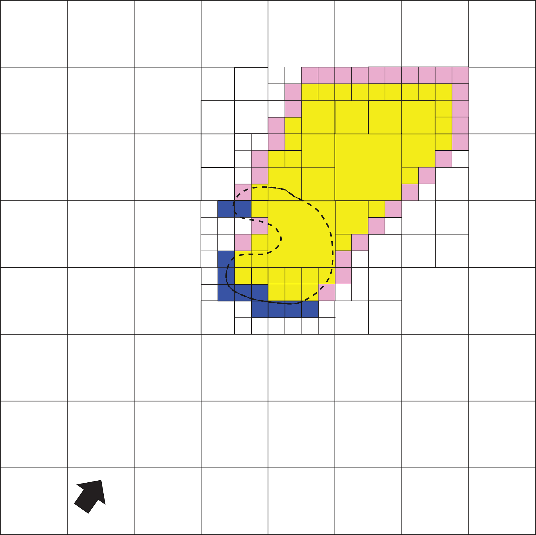
Voxel labels. Occupied voxels are marked in blue, unknown voxels in yellow, and VUVs in pink. VUV: visible unknown voxel.

General workflow

In general, the 3-D reconstruction of an object is an iterative process of sensing and deciding where to move and see next. Algorithm 1 resumes the workflow which is described below.

Algorithm 1

3-D object reconstruction method. It receives the initial robot state, x _init, and the object bounding box, W _box, then it reconstructs the object and returns the object point cloud P _obj.

The reconstruction requires the object bounding box, W_box, and the initial state, x_init, from where the object is visible. Based on W_box, the partial model, M, is initialized by setting all the voxels inside M as unknown. Then, the robot moves to the given state and an observation is made. The observed point cloud (z) is registered to the incremental point cloud of the object, P_obj, using the iterative closest point algorithm.²⁶ During the registration, z is aligned and P_obj is increased. Next, the aligned point cloud, z′, updates the partial model. Then, the next robot state is planned with the ORT. If the ORT returns a valid state and the stop criterion has not been satisfied then the process is repeated.

ORT construction

To compute the NBVS, we propose the ORT. The method is based on the RRT. The original RRT method is an algorithm that is designed for efficiently searching non-convex high-dimensional configuration or state spaces¹³; it grows a tree structure in the collision-free space, each vertex represents a possible state, and each edge represents the control that makes the robot move between vertices. RRT can be considered as a Monte Carlo way of biasing search into largest Voronoi regions. RRT and derived methods have been used in a variety of applications, for instance, motion planning for humanoid robots.²⁷

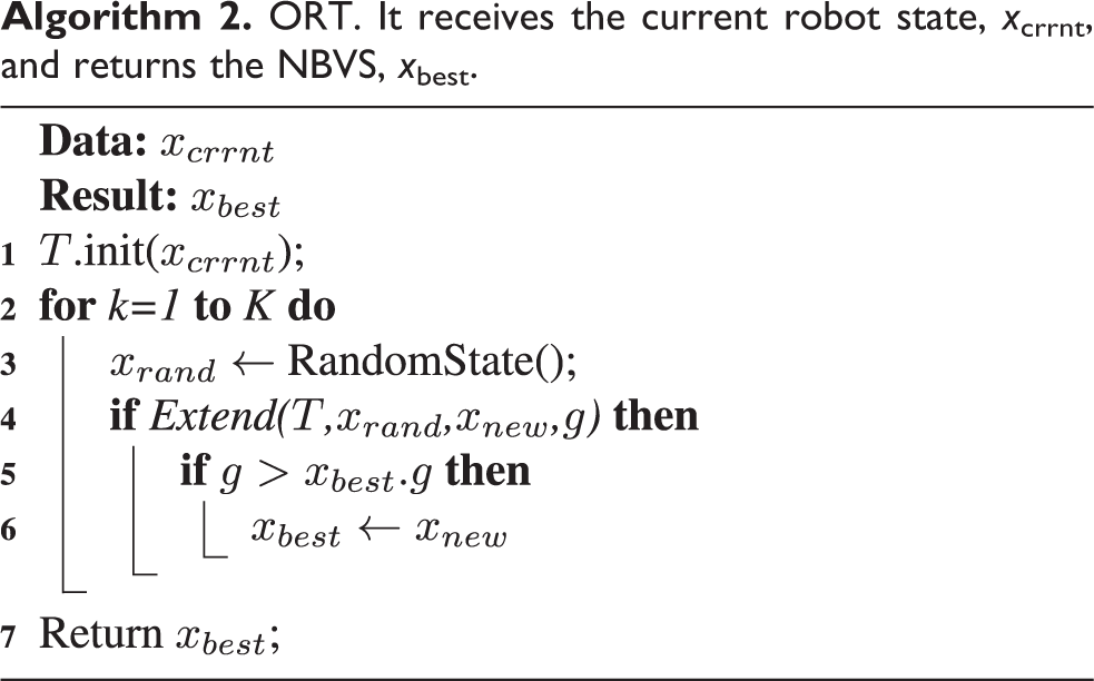
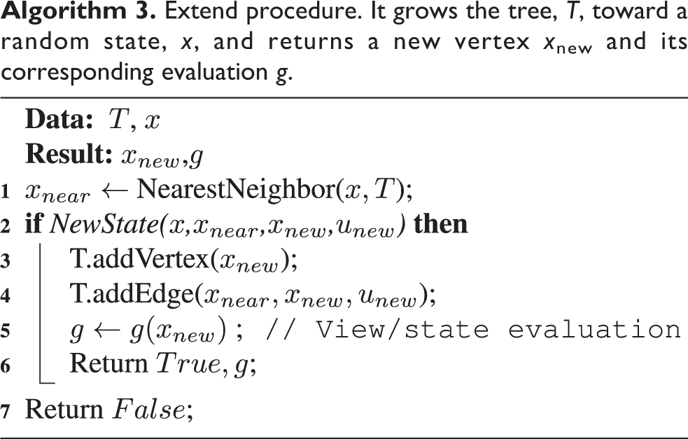
The ORT grows in the state space in the same way that an RRT does, but instead of trying to reach a goal state, the ORT grows until K iteration is met. During the growing, each added vertex is tested with a utility function. At the end, the NBVS is the vertex with the highest evaluation. Algorithm 2 resumes the ORT method. In detail, the ORT grows from an initial state x_crrnt which is the current robot state. Then, a random state, x_rand, is generated, line 3. The extend procedure (Algorithm 3) grows the tree in the direction of x_rand; if the extension operation is successful, the utility, g, of the new vertex is returned. The utility is calculated according to the evaluation described in section “View/state evaluation.” If the utility g is higher than the previous evaluated vertices then x_new is kept as the NBVS (x_best).

Algorithm 2

ORT. It receives the current robot state, x _crrnt, and returns the NBVS, x _best.

Algorithm 3

Extend procedure. It grows the tree, T, toward a random state, x, and returns a new vertex x _new and its corresponding evaluation g.

We have selected the RRT to guide the search for several reasons. It rapidly extends in the state space and with enough vertices it can reach any state (within a certain gap and for reachable states). It allows us to determine the NBVS directly in the state space. We are sure that the candidate states are collision free and reachable given that they are demonstrated properties of the RRT.¹³ In addition, we can easily calculate the distance from the current state using the tree path.

View/state evaluation

The utility function ranks the candidate states according to their goodness for the reconstruction process. Formally, let $g : X \to ℝ$ be the utility function. We use the utility function proposed by Vasquez et al., which is a product of four factors, see equation

g (x) = p (x) \cdot r (x) \cdot d (x) \cdot I (x)

Each factor evaluates a particular constraint of the problem and they are explained below. We implement this function because it allows us to evaluate the factors in cascade, making the evaluation faster. Furthermore, we are proposing a new information metric.

Positioning

p(x) is 1 when the robot state is collision free, and a collision-free path from the current state to the evaluated state is available; otherwise it is 0. This factor has been written in equation (1) to keep the notation described in the previous articles. However, notice that it is no longer needed since the ORT verifies collision after the extension process.

Registration

To register the new scan, previous works have proposed to assure a minimum amount of overlap or consider all causes of failure.²⁸ In this work, we use the registration factor proposed by Vasquez et al., where r(x) is 1 if a minimum percentage of overlap with previous surfaces exists, and 0 otherwise. Such percentage is calculated by dividing the number of occupied voxels per the sum of occupied voxels plus the number of visible unknown voxels (VUVs).

Distance metric

The distance factor, d(x), assesses a state depending on how far it is from the current robot state. The inclusion of this factor has given evidence that it helps to decrease the total traveled distance of the reconstruction and helps to decrease the position uncertainty.¹¹ Some examples of distance factors are an orthodromic distance for free fliers,⁵ a cost that measures the robot path,¹² or a decrement relative to the cost.²⁵ It is worth to say that d(x) requires to be tuned depending on the robot platform and user needs. During the experiments, this factor was set to 1 to reduce the number of addressed variables. A comparison between distance metrics is left for future work.

Information metric

The information metric, I(x), is a function that receives a state and returns a numeric value according to how much new relevant information about the object can be acquired. In this section, we describe a new information metric, called FIG, alongside several reported metrics that are used in the experiments section.

A necessary step for the calculation of the information metric is the ray tracing. It retrieves from the partial model the set of voxels that will be observed by the sensor; in other words, it is a simulation of the scan inside the probabilistic octree. As a result, for each ray, r, of the sensor, R, a set of voxels M_r is obtained. See the work of Amanatides and Woo²⁹ for more details on ray tracing.

Frustum information gain

The FIG is a variant of the information gain metric used by Kriegel et al.² and Isler et al.²⁵ This approach is based on the asseveration that the information contained in each voxel i can be measured by its entropy,² see equation

I (i) = \sum_{i \in f (x)} - p (i) ln (p (i)) - (1 - p (i)) ln (1 - p (i))

where p(i) is the occupancy probability for the voxel i.

The entropy of a voxel, equation (2), is higher when the probability of been occupied is close to 0.5, and it is lower when the probability tends to 0 or 1. Namely, the voxel has more information when it is unknown. Therefore, the FIG sums all the information that is contained in the set of unknown voxels that lie inside the sensor frustum, see equation

I_{f} (x) = \sum_{\forall i | i \in f (x) \land i \in M_{u}} I (i)

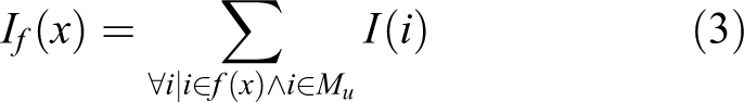
where f(x) is the set of voxels that are touched by the ray tracing

f (x) = \underset{\forall r \in R_{x}}{\cup} M_{r}

and M_u is the set of unknown voxels.

Figure 3 shows an example of the voxels that contribute to the FIG. Unlike Kriegel’s metric, FIG integrates the entropy for each voxel inside the sensors frustum but avoids multiple integration caused by ray tracing,

Figure 3.

Example of FIG. The figure shows in green, the voxels that contribute to the FIG. Each touched voxel contributes only one time to the metric. FIG: frustum information gain.

Scan information gain

The metric, proposed by Kriegel et al.,² calculates the information gain for all voxels touched by the rays of the sensor, see equation (5). Unlike the FIG, in this method, each ray contributes to the computation even if the voxels are touched more than one time (see Figure 4)

I_{s} (x) = \sum_{\forall r_{j} \in R_{x}} \sum_{\forall i \in M_{r_{j}}} I (i)

Figure 4.

Multiple contribution of the same voxel. SIG metric adds for each ray that is traced, causing that the voxels nearest to the sensor will be counted many times. In the figure, as the voxel is counted multiple times, it increased its green saturation. SIG: scan information gain.

Visible unknown voxels

This approach counts the VUVs, see equation (6). According to the study by Vasquez-Gomez et al.,¹¹ the VUVs are the unknown voxels that are first touched by the ray tracing. In the study by Vasquez-Gomez et al.,⁵ the same type of voxels is called occplane (the contraction of occlusion plane) and they are defined as unknown voxels that are adjacent to a free voxel

I_{u} (x) = \sum_{i \in f (x)} I_{o} (i)

So that

I_{o} (i) = {\begin{matrix} 1 & i is a visible unknown voxel \\ 0 & i otherwise \end{matrix}

Rear side voxel

This metric counts the number of voxels behind a seen surface expecting that such voxels will be part of the object, see equation (8). This metric was proposed by Isler et al.²⁵ and it shows a surface coverage advantage with respect to other metrics. See the work of Isler et al.²⁵ for more details.

I_{r} (x) = \sum_{\forall r_{j} \in R_{x}} \sum_{\forall i \in M_{r_{j}}} I_{b} (i)

where

I_{b} (i) = {\begin{matrix} 1 & i is a rear side voxel \\ 0 & i otherwise \end{matrix}

Stop criterion

There are two questions related to the stop criterion: (i) when the ORT should stop growing? and (ii) when the reconstruction should be stopped? In this article, we answer the former question by setting a maximum number of iterations, k. However, an alternative is to have an estimate of the NBVS goodness and then to stop the ORT when the evaluation of the added vertex, x_new, is close to the estimation. Such estimation can be obtained with a synthesis method.³ The latter question is more difficult to answer. It is possible to know when the object is complete,¹⁰ in that case, the reconstruction is stopped. However, if there is no path to the NBVS, the algorithm can run forever given that the RRT is a probabilistic complete algorithm but it cannot detect an unreachable goal.¹³

Experiments

We present several experiments that analyze the proposed tree-based search method. The questions that we want to answer are how does the amount of ORT vertices affect the reconstruction coverage? is the ORT better than the RS proposed in a previous approach? What information metric is best suited for the ORT?

The experiments were made using view planning library which is available as an open source under BSD license (https://github.com/irvingvasquez/vpl). Please see an example of the experiments at the online video: https://youtu.be/zLpubkJc_bc.

Performance metrics

Surface coverage. It is computed as the ratio of correspondent points over the total number of points in the ground truth model; a correspondent point is a ground truth point closer than a threshold (3 mm) to a built model point.¹¹

Coverage increment. The coverage increment is the surface coverage difference between two consecutive scans

Δ c = c_{i} - c_{i - 1}

Observation cost. It quantifies the applied resources to complete an iteration of the reconstruction. To span all the different processes in one single metric, we use the processing time. So that

Δ_{t} = t_{plan} + t_{mov} + t_{update}

where t_plan is the lapse of time to compute the NBVS, t_mov the lapse to reach the NBVS, and t_update the lapse to take the scan, register the point cloud, and update the octomap.

Reconstruction efficiency. It calculates the rate of change in coverage with respect to the cost, namely, the amount of surface that is increased per unit of time.

ζ = Δ c / Δ t

Reconstruction scene configuration

The reconstruction scene is composed of the object, in the center of the scene, and a mobile manipulator robot with an eye in hand sensor (see Figure 5). The mobile manipulator robot has eight degrees of freedom, three in the differential drive base (A MobileRobots Patrol Bot) and five in the arm (Neuronics Katana). The sensor is a time-of-flight camera with 176 × 174 points. The voxel resolution for all the experiments is 2 cm.

Figure 5.

Reconstruction scene. (a) Initial scene. (b) Octree after the first scan.

Effect of the ORT size on the coverage

The objective of this experiment is to observe the impact that the tree size (k vertices) has on the surface coverage. In addition, we want to identify an adequate k threshold that shows a good trade-off between coverage and computational cost. So, we have reconstructed an object 10 times for five different values of k; $k = 2.5 \times 10^{3}, 5 \times 10^{3}, 10 \times 10^{3}, 20 \times 10^{3}, 40 \times 10^{3}$ . Notice that the amount of vertices is doubled each time.

The object to be reconstructed is the Stanford bunny³⁰ which has been placed on a table (Figure 5). The information metric used in this experiment was VUV. The stop criterion of the reconstruction is 25 iterations or when none of the vertices provides new information. Distance factor was set to 1 to decrease the variables of the experiment. NBVS computation times per iterations were 176 s, 192 s, 220 s, 564 s, and 1364 s, respectively.

First, we analyze the surface coverage. Figure 6 displays the reconstruction coverage. It shows only the first 15 iterations, because in some cases (with a large k), the reconstruction ends before the 25th iteration. We observe that as the number of vertices is increased, the reconstruction effectiveness, in terms of coverage, is also increased. However, the experiment suggests that such effectiveness approaches to a limit, noticing that the coverage using 40 × 10³ vertices is similar to the coverage using 20 × 10³ even that the number of vertices is doubled. We also found that the length of the trajectories to the NBVS increases as the amount of vertices increases (see Figure 7); the reason for this fact is that with a larger k, a better NBVS is found; however, it is usually further with respect to the current robot state.

Figure 6.

Mean surface coverage that is reached using different amounts of vertices (k) in the ORT. We observe that as the number of vertices is increased, the effectiveness of the ORT, in terms of reconstruction coverage, is increased. ORT: object reconstruction tree.

Figure 7.

Mean length of the trajectories to the NBVS using different amounts of vertices (k) in the ORT. The experiment shows that usually the length of the trajectory to the NBVS is larger as the ORT grows, given that it usually finds the NBVS in a further state. NBVS: next best view/state; ORT: object reconstruction tree.

Second, we analyze the reconstruction efficiency (see Figure 8). We notice that a small or too large k provides a poor efficiency. This phenomenon is due to the fact that small trees have a short processing time but poor coverage, due to the short expansion of the tree (see Figure 9(a)). On the other hand, a large tree provides good coverage but it will consume large processing times (see the tree in Figure 9(e)). So there is a trade-off between coverage and processing time. In this experiment, 10 × 10³ vertices show a good trade-off.

Figure 8.

Reconstruction efficiency. The experiment provides evidence that, at the initial iterations, investing more time in searching a better NBVS could not be the best deal, given that the coverage efficiency is decreased. NBVS: next best view/state.

Figure 9.

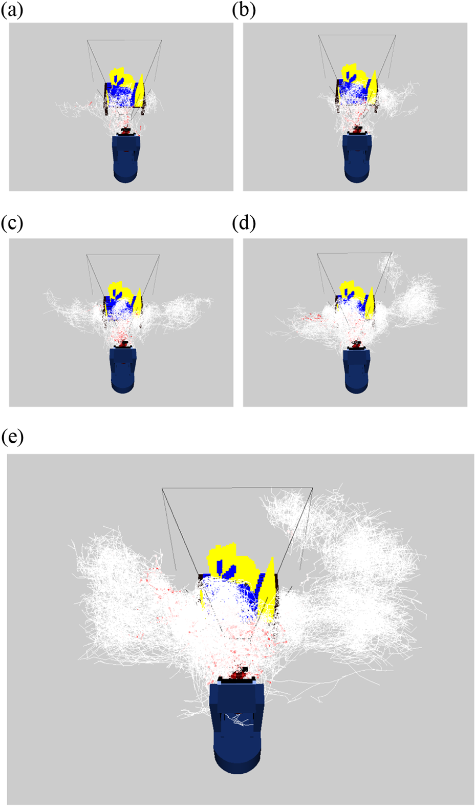
Projection of the end-effector poses for each vertex in the ORT. The red points are the poses with higher evaluation. (a) ORT with 2.5 × 10³ vertices, (b) ORT with 5 × 10³ vertices, (c) ORT with 10 × 10³ vertices, (d) ORT with 20 × 10³ vertices, and (e) ORT with 40 × 10³ vertices. ORT: object reconstruction tree.

Additionally, we have found that in early stages of the reconstruction, the NBVS is usually close to the current robot state; see in Figure 9 that even when the number of vertices is increased, the best-evaluated poses are close to the current robot state. So, to improve the reconstruction efficiency, we recommend a small tree in early iterations. On the other hand, at the latest iterations, a large tree may be needed given that the NBVS could be far from the current robot state.

During the experiments, we have observed that while the tree is expanding in the state space, in the work space, the poses of the sensor are not been distributed uniformly (see the snapshots in Figure 9). This phenomenon is caused by the redundancy of the system.

ORT versus RS

In the previous work,¹² an NBVS planning method based on RS was proposed. In this experiment, we compare the ORT with that approach. The main difference between approaches is that while the RS makes a uniform sampling of the state space and tries to connect the best-evaluated states, the ORT evaluates the vertices that are added to the tree. In this experiment, the number of samples for RS was 20 × 10³, and the value for k, the tree size, was also 20 × 10³. Ten reconstructions per approach were done. The object reconstructed was the bunny. The information metric was VUV. The stop criterion was 25 scans and the distance factor was set to 1 to decrease the variables of the experiment.

The results, condensed in Figure 10, show that the ORT beats the performance of RS. The reason for this phenomenon is that the ORT is adding states that are relatively close to the current state; such states are promising because likely they will observe some new surface but surely they will satisfy the registration constraint. On the other hand, the RS could provide states that are better in terms of information but they could not satisfy the registration constraint since they could be too far from the current robot state; furthermore, such samples cannot be always reached with the RRT. In the study by Vasquez et al.,¹² a similar performance of the ORT was obtained but 100 × 10³ samples were required.

Figure 10.

Comparison of the ORT versus RS. Both methods were set with 20 × 10³ samples. ORT beats the RS for the reconstruction of the bunny object, see the text for more details. ORT: object reconstruction tree; RS: random sampling.

Information metrics comparison

In this experiment, we compare the performance of the proposed FIG against several state-of-the-art metrics. The objective is to get evidence of what metric is best suited for the ORT. In this experiment, the bunny object was reconstructed using an ORT of 20 × 10³ nodes. Distance factor was set to 1 to decrease the variables of the experiment. The information factor of the utility function was replaced by each metric described in section “Information metric.” Ten reconstructions were run for each metric. Figure 11 shows the surface coverage for each metric. Figure 12 shows the remaining unknown volume inside the object bounding box.

Figure 11.

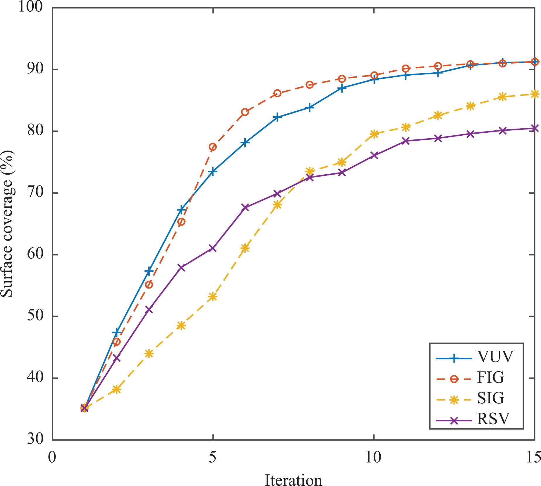
Information metrics comparison based on the coverage. The figure shows the mean surface coverage that is reached per iteration. See the text for more details.

Figure 12.

Information metrics comparison based on the remaining unknown volume. The figure shows the amount of unknown volume that is left inside the bounding box per iteration.

The experiments show that FIG and VUV metrics have better performance over the scan information gain (SIG) and rear side voxel (RSV) metrics. This phenomenon is due to the fact that the former metrics “counts” over unrepeated touched voxels, unlike the latter metrics that could count one single voxel multiple times, comparing equation (3) versus equation (5). Therefore with SIG and RSV metrics, the robot tends to get the sensor close to the unknown volume because this behavior gets better evaluations but some voxels are counted many times for different rays of the ray tracing (see Figure 4). The situation for SIG and RSV metrics gets worse because when the sensor is too close to the unknown volume, where it is more difficult to the ORT to get out from that state (it can easily collide with the object or table). On the other hand, FIG and VUV metrics tend to put more voxels inside the sensor frustum; this behavior provokes a higher surface coverage. With respect to the remaining unknown volume, RSV metric shows a poor performance given that, in some cases, clusters of unknown volume are not seen by the sensor during the reconstruction, given that, some of those clusters do not have occupied voxels and by definition they do not contain rear side voxels (see the Online Supplementary Material).

The difference between metrics found in this experiment has not been reported in previous articles,^11,25 because the set of evaluated views is usually restricted, for example, a convenient distance to the object could be fixed during the view/states generation. In this article, the ORT is in charge of generating such view/states.

Experiment analysis

The experiments provide evidence that the ORT is capable of reconstructing an unknown object. In addition, the method has shown a better performance against an RS scheme for the same number of samples (vertices). We also have found that in the early iterations of the reconstruction, a large tree that spans the state space and finds a better evaluated NBVS is not necessarily the best, given that the reconstruction efficiency is compromised. Therefore, we recommend that in early iterations, a small tree will be grown; it will provide in a short computation time an NBVS that is close to the current robot state, improving the reconstruction efficiency. On the other hand, the proposed FIG metric has shown a better performance with respect to the state-of-the-art metrics. In the experiment, we have observed that FIG metric tends to cover bigger unknown volumes; in consequence, the object is reconstructed faster. A current drawback of the whole method is the large computation time, given that each vertex of the tree is evaluated and we are using a detailed voxel resolution; however, this issue can be addressed using some strategies like hierarchical ray tracing, parallel processing, or reconfigurable hardware implementations. Finally, we remark that this method is better suited for robots with many degrees of freedom whose inverse kinematics is not trivial; otherwise, surface-based methods could perform better.

Future research directions are (i) to adjust the ORT growing depending on the partial model state. We believe that in early iterations, only a small tree is needed to find a good NBVS, given that the unknown voxels can be reached even with a small sensor movement, while for the last iterations, a large tree should be required and (ii) to bias the ORT exploration in order to explore the view space instead of exploring the state space.

Conclusions and future work

The ORT method for computing the NBVS for 3-D object reconstruction was presented. The ORT explores the robot’s state space using a tree structure; each vertex that is added to the tree is evaluated depending on how much it contributes to the reconstruction. The vertex with the highest evaluation is selected as the next view/state. The method is able to compute the NBVS and its corresponding collision-free trajectory directly in the state space avoiding inverse kinematics calculation. Furthermore, we have presented a new information metric, called FIG. The FIG avoids the multiple counting of voxels that is made by previous metrics. The experiments shown that the method is capable of reconstructing an arbitrary object even with the use of a non-holonomic robot of eight degrees of freedom. The experiments also shown that the proposed information metric improves the reconstruction performance, given that, by not making multiple counting, the sensor’s frustum is filled with a bigger amount of unknown voxels. A drawback of the method is that it requires high computational resources when for very fine resolutions, however, parallel programming or hierarchical ray tracing can be used to reduce the computation time.

In a future work, we will extend the ORT to optimal motion planning and uncertainty during the execution of the planned trajectories. In addition, we would like to investigate strategies to bias the ORT exploration to the view space instead of exploring the state space.

Footnotes

Acknowledgment

The authors would like to thank CONACYT.

Declaration of conflicting interests

The author(s) declared no potential conflicts of interest with respect to the research, authorship, and/or publication of this article.

Funding

The author(s) disclosed receipt of the following financial support for the research, authorship, and/or publication of this article: This work was supported by CONACYT for the project cátedra 1507.

ORCID iD

J Irving Vasquez-Gomez

References

Scott

Roth

Rivest

. View planning for automated three-dimensional object reconstruction and inspection. ACM Comput Surv 2003; 35: 64–96. DOI:10.1145/641865.641868.

Kriegel

Rink

Bodenmuller

. Next-best-scan planning for autonomous 3d modeling. In: Proceedings IEEE/RSJ international conference on intelligent robots and systems, Vilamoura, Algarve, Portugal, 7–12 October 2012, pp. 2850–2856. IEEE. DOI:10.1109/IROS.2012.6385624.

Chen

. Vision sensor planning for 3-D model acquisition. IEEE Trans Syst Man Cybern 2005; 35(5): 894–904.

Zhang

Miao

. Determining next best view based on occlusion information in a single depth image of visual object. Int J Adv Robot Syst 2017; 14(1): 1–11. DOI:10.1177/1729881416685672.

Vasquez-Gomez

Lopez-Damian

Sucar

. View planning for 3D object reconstruction. In: Proceedings IEEE/RSJ international conference on intelligent robots and systems, St. Louis, MO, USA, 10–15 October 2009, pp. 4015–4020.

Cieslewski

Kaufmann

Scaramuzza

. Rapid exploration with multi-rotors: a frontier selection method for high speed flight. In: IEEE/RSJ international conference on intelligent robots and systems (IROS), Vancouver, BC, Canada, 24–28 September 2017, pp. 2135–2142. IEEE.

Doumanoglou

Kouskouridas

Malassiotis

. Recovering 6D object pose and predicting next-best-view in the crowd. In: 2016 IEEE conference on computer vision and pattern recognition, Las Vegas, NV, USA, 27–30 June 2016, pp. 3583–3592.

Chen

Zhang

. Active sensor planning for multiview vision tasks. Berlin, Heidelberg: Springer-Verlag, 2008.

Karaszewski

Adamczyk

Sitnik

. Assessment of next-best-view algorithms performance with various 3D scanners and manipulator. ISPRS J Photogramm Remote Sens 2016; 119: 320–333. DOI:10.1016/j.isprsjprs.2016.06.015.

10.

Torabi

Gupta

. An autonomous six-DOF eye-in-hand system for in situ 3D object modeling. Int J Robot Res 2012; 31(1): 82–100.

11.

Vasquez-Gomez

Sucar

Murrieta-Cid

. View/state planning for three-dimensional object reconstruction under uncertainty. Auton Robot 2015; 41: 89–109. DOI:10.1007/s10514-015-9531-3.

12.

Vasquez

Sucar

Murrieta-Cid

. View planning for 3D object reconstruction with a mobile manipulator robot. In: Proceedings IEEE/RSJ international conference on intelligent robots and systems, Chicago, IL, USA, 14–18 September 2014, pp. 4227–4233.

13.

LaValle

Kuffner

. Randomized kinodynamic planning. Int J Robot Res 2001; 20(5): 378–400.

14.

Chen

Kwok

. Active vision in robotic systems: a survey of recent developments. Int J Robot Res 2011; 30(11): 1343–1377. DOI:10.1177/0278364911410755.

15.

Maver

Bajcsy

. Occlusions as a guide for planning the next view. IEEE Trans Pattern Anal Mach Intell 1993; 15: 417–433. DOI: 10.1109/34.211463.

16.

Pito

. A solution to the next best view problem for automated surface acquisition. IEEE Trans Pattern Anal Mach Intell 1999; 21(10): 1016–1030. DOI:10.1109/34.799908.

17.

Connolly

. The determination of next best views. In: Proceedings IEEE international conference on robotics and automation, Vol. 2. St. Louis, MO, USA, 25–28 March 1985, pp. 432–435.

18.

Foissotte

Stasse

Escande

. A two-steps next-best-view algorithm for autonomous 3D object modeling by a humanoid robot. In: Proceedings IEEE international conference on robotics and automation, Kobe, Japan, 12–17 May 2009, pp. 1078–1083. ISBN 978-1-4244-2788-8.

19.

Hornung

Wurm

Bennewitz

. Octomap: an efficient probabilistic 3D mapping framework based on octrees. Auton Robot 2013; 34(3): 189–206. DOI:10.1007/s10514-012-9321-0.

20.

Tarabanis

Allen

Tsai

. A survey of sensor planning in computer vision. IEEE Trans Robot Autom 1995; 11: 86–104.

21.

Monica

Aleotti

. Contour-based next-best view planning from point cloud segmentation of unknown objects. Auton Robot 2017; 1–16. DOI:10.1007/s10514-017-9618-0.

22.

Oriolo

Vendittelli

Freda

. The SRT method: randomized strategies for exploration. In: IEEE international conference on robotics and automation, Vol. 5, New Orleans, LA, USA, 26 April–1 May 2004, pp. 4688–4694. IEEE.

23.

Torabi

Kazemi

Gupta

. Configuration space based efficient view planning and exploration with occupancy grids. In: IEEE/RSJ international conference on intelligent robots and systems, San Diego, CA, USA, 29 October–2 November 2007, pp. 2827–2832.

24.

Bircher

Kamel

Alexis

. Receding horizon “next-best-view” planner for 3D exploration. In: 2016 IEEE international conference on robotics and automation (ICRA), Stockholm, Sweden, 16–21 May 2016, pp. 1462–1468. DOI:10.1109/ICRA.2016.7487281.

25.

Isler

Sabzevari

Delmerico

. An information gain formulation for active volumetric 3D reconstruction. In: 2016 IEEE international conference on robotics and automation, Stockholm, Sweden, 16–21 May 2016, pp. 3477–3484. IEEE.

26.

Besl

McKay

. A method for registration of 3-D shapes. IEEE Trans Pattern Anal Mach Intell 1992; 14: 239–256. DOI:10.1109/34.121791.

27.

Kuffner

Nishiwaki

Kagami

. Motion planning for humanoid robots. In: Proceedings the eleventh international symposium on robotics research. Siena, Italy, 2003, pp. 365–374. Berlin, Heidelberg: Springer.

28.

Low

Lastra

. An adaptive hierarchical next-best-view algorithm for 3D reconstruction of indoor scenes. In: Proceeding 14th pacific conference on computer graphics and applications, Taipei, Taiwan, October 2006, pp. 1–8.

29.

Amanatides

Woo

. A fast voxel traversal algorithm for ray tracing. In: Eurographics, August, 1987, pp. 3–10.

30.

Levoy

Gerth

Curless

. The Stanford 3D scanning repository, 2005. URL http://www-graphics.stanford.edu/data/3dscanrep (accessed september 2017).

Tree-based search of the next best view/state for three-dimensional object reconstruction

Abstract

Keywords

Introduction

Related work

Contributions

The ORT

Assumptions and concepts

General workflow

ORT construction

View/state evaluation

Positioning

Registration

Distance metric

Information metric

Frustum information gain

Scan information gain

Visible unknown voxels

Rear side voxel

Stop criterion

Experiments

Performance metrics

Reconstruction scene configuration

Effect of the ORT size on the coverage

ORT versus RS

Information metrics comparison

Experiment analysis

Conclusions and future work

Footnotes

Acknowledgment

Declaration of conflicting interests

Funding

ORCID iD

References