Control of Open Contour Formations of Autonomous Underwater Vehicles

Abstract

In this paper, we propose a distributed elastic behaviour for a deformable chain-like formation of small autonomous underwater vehicles with the task of forming special shapes which have been explicitly defined or are defined by some iso-contour of an environmental concentration field. In the latter case, the formation has to move in such a way as to meet certain formation parameters as well as adapt to the iso-line. We base our controller on our previous models (for manually controlled end points) using general curve evolution theory but will also propose appropriate motions for the end robots of an open chain.

1. Introduction

Exploration and mapping of the underwater environment using autonomous vehicles has gained a lot of momentum in the past decade. Numerous robotic platforms have been designed, fabricated and used for practical purposes. One important aspect of mapping is to identify and track boundaries of environmental features. These, in particular, include isolines (level curves) of concentration fields (such as temperature or salinity) (Okubo, A., 1980) as well as bathymetric contours. In (Bennett, A., Leonard, J.J., 2000), a single vehicle tracks bathymetric contours provided by an altitude map (the robot marked 1 in figure 1). Due to inherent limitations of a single vehicle, multi-robot systems have been proposed and studied in recent years, although real-world implementations still lag behind.

In (Ogren, P., Leonard, N.E., 2002) and (Ogren, P., Fiorelli, E., Leonard, N.E., 2004), a small group of robots form special shapes, suitable for estimating local gradients, and localize the source of the field (formation marked 2 in figure 1). In (Zhang, F., Leonard, N.E., 2005), a formation of four robots converge to and track a desired isoline (formation 3 in figure 1), creating contour maps of the environment. These approaches are not scalable. The latter one, although addressing boundary tracking, suffers from the same limitations as the single robot case.

Fig. 1:

Adaptation to contours

In (Robinett, R.D., Hurtado, J.E., 2004), an arbitrary number of robots individually localize and move to a source by field gradient estimation, attaining a particular formation at the source. The setting in (Christopoulos, V., Roumeliotis, S., 2005) is similar but they are mainly interested in estimating parameters of the diffusion process. There is no tight coupling between the robots in these two approaches and cooperation is not explicitly defined.

(Gazi, V., Passino, K.M., 2002) studies large swarms of mobile sensors but their approach is more suitable for modelling animal flocks (group marked 4). (Cortes, J., Martinez, S., Bullo, F., 2004) and (Belta, C., Kumar, V., 2002), among others, study large assemblies of robots, especially suitable for covering extended areas. Finally, (Zarzhitsky, D., Spears, W., Spears, W., 2005) use fluxotaxis with relatively large number of robots for source localization. This list is not exhaustive but is indicative of the state of the art.

On the other hand, the approach studied in (Kalantar, S., Zimmer, U., 2005a), (Kalantar, S., Zimmer, U., 2005b), (Kalantar, S., Zimmer, U., 2006a), and (Marthaller, D., Bertozzi, A.L., 2002) is, in our opinion, a more natural choice for the task of boundary tracking. These specific types of formation are composed of a chain of mobile platforms, cooperatively moving towards the feature of interest, mimicking an elastic band. Apart from being especially suited to isoline tracking, the method is scalable and lends itself to distributed control strategies. We dubbed them contour formations in previous publications (formation 5 in figure 1). The idea, that of evolving an elastic band in such a way that it eventually adapts to a boundary was originally suggested by machine vision researchers in (Caselles, V., Kimmel, R., Sapiro, G., 1997) for segmentation but, nevertheless, the same abstract model can be used for our purposes. This, in turn, inspired the authors of (Marthaller, D., Bertozzi, A.L., 2002) to apply the same concept to robotics straightforwardly. We took this idea further in previous publications, focusing on the problem from a robotics point of view. It should be mentioned that the approach proposed in (Michael, N, Kumar, V., 2005) is very similar but it lacks the elegant inter-robot interaction which is provided by curve evolution schemes.

Here, we will first review the basic concepts, summarize the control scheme developed in (Kalantar, S., Zimmer, U., 2006b) for formations with fixed end points and then propose appropriate motions for free-moving boundary robots. Simulation runs show the effectiveness of the approach.

As in previous papers, we will use Serafina (the autonomous underwater vehicle developed at our lab and shown in figure 2) as the model. To make the presentation simpler, it is assumed that the vehicles are capable of tracking a desired trajectory with negligible dynamics. Thus, the motion of a robot R, with position q, is described by ̇q = τ(q, t), where τ(q, t) represents the designed trajectory. It is also assumed that the robots are individually capable of measuring the local gradient of the field V_qF(q).

Fig. 2:

Serafina

2. Contour formations

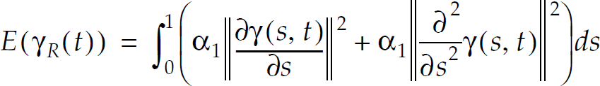
It turns out to be beneficial to model a contour formation by a continuous curve ${\gamma }_R:[0,1]\times T\to {\mathrm{\Re }}^2$ , in the plane, parametrized by s, with boundary condition γ _R (0, t) = γ _R (1, t), for a closed curve, and γ _R (0, t) = γ _R (1, t) = 0, for an open curve, for all t ≥ t₀. Such a curve should ideally act like an elastic band being deformed by an external force Δ_xF(x) which is the local gradient of a concentration field $F:{\mathrm{\Re }}^2\to \mathrm{\Re }$ . As will be seen shortly, a recipe for realizing such behaviour will lead to a distributed control scheme for contour formations. The most general motion for a curve is

$$\dot{{\gamma }_R}(s,t)={\eta }_N(s,t)\stackrel{\rightharpoonup }{N}(s,t)+{\eta }_T(s,t)\stackrel{\rightharpoonup }{T}(s,t)$$

(1) where $\stackrel{\rightharpoonup }{T}(s,t)=\dot{{\gamma }_R}(s,t)/\parallel \dot{{\gamma }_R}(s,t)\parallel$ is the unit tangent vector and $\stackrel{\rightharpoonup }{N}(s,t)$ (the unit normal vector) is such that $(\stackrel{\rightharpoonup }{N}(s,t),\stackrel{\rightharpoonup }{T}(s,t))$ form a basis for ${\mathrm{\Re }}^2$ . Note that, for open curves, these vectors are not defined. Now note that the tangential velocity only changes the parametrization and has no effect on the image of the curve.

η_N(s, t) should include internal as well as external forces:

$${\eta }_N(s,t)=\beta ={\beta }_{1}I(s,t)-{\beta }_{2}E(s,t)$$

(2)

Among the models proposed are the traditional elastic snake model

$$\begin{array}{rl}& I_S(s,t)=({\alpha }_1\frac{{\mathrm{\partial }}^2}{\mathrm{\partial }{s}^2}{\gamma }_R(s,t)-{\alpha }_2\frac{{\mathrm{\partial }}^4}{\mathrm{\partial }{s}^4}{\gamma }_R(s,t))\cdot \stackrel{\rightharpoonup }{N}(s,t)\\ & E_S(s,t)={\mathrm{\nabla }}_{{\gamma }_R(s,t)}F({\gamma }_R(s,t))\cdot \stackrel{\rightharpoonup }{N}(s,t)\end{array}$$

(3) and the one based on general curve evolution

$$I_C(s,t)=g(F({\gamma }_R(s,t))-F_d\kappa (s,t)$$

(4)

$$E_C(s,t)=\dot{g}(F({\gamma }_R(s,t))-F_d)E_S(s,t)$$

(5) where

$$\kappa (s,t)=\frac{(\mathrm{\partial }/\mathrm{\partial }s)({\gamma }_R(s,t))\times ({\mathrm{\partial }}^2/\mathrm{\partial }{s}^2)({\gamma }_R(s,t))}{\parallel (\mathrm{\partial }/\mathrm{\partial }s)({\gamma }_R(s,t)){\parallel }^3}$$

(6) is the curvature at γ _R (s, t). g(·) goes to zero as F(γ _R (s, t)) → F_d. F(q) = F_d defines a level set which we represent with the curve ${\gamma }_{F_d}:[0,1]\to {\mathrm{\Re }}^2$ . In the snake formulation, special balloon forces are used, depending on whether the closed curve is inside the level curve or not. The snake equation is the gradient descent for the energy functional

$$E({\gamma }_R(t))={\int }_0^1({\alpha }_1{\parallel \frac{\mathrm{\partial }\gamma (s,t)}{\mathrm{\partial }s}\parallel }^2+{\alpha }_1{\parallel \frac{{\mathrm{\partial }}^2}{\mathrm{\partial }{s}^2}\gamma (s,t)\parallel }^2)ds$$

while the equation for curve evolution minimizes ${\int }_0^{1}g(\gamma (s,t))ds$ . We will base our methods on the more general curve evolution model. Translating back to the case of a collection R of robots R_i, i = 0, …, N − 1, with positions $q_i\in {\mathrm{\Re }}^2$ , measured with respect to an inertial coordinate system γ, we will have the general for

$$\begin{array}{rl}& {\dot{q}}_i(t)={\eta }_{N_i}(t){\stackrel{\rightharpoonup }{N}}_i(q_{i-1}(t),q_{i+1}(t))\\ & \hspace{0.17em}+{\eta }_{T_i}(q_i(t),q_{i-1}(t),q_{i+1}(t)){\stackrel{\rightharpoonup }{T}}_i(q_{i-1}(t),q_{i+1}(t))\end{array}$$

(7)

$${\eta }_i(t)={\eta }_{N_i}(q_i(t),q_{i-1}(t),q_{i+1}(t),{\mathrm{\nabla }}_{q_i(t)}F(q_i(t)))$$

(8) is a function of the discrete curvature. An estimate for curvature is given by

$${\kappa }_i(t)=sign(⟨q_{i+1}-q_i,q_i-q_{i-1}⟩)|{\kappa }_i(t)|$$

(9) where

$$|{\kappa }_i(t)|=\frac{1}{\parallel q_{i+1}-q_{i-1}\parallel }\text{acos}\left(\frac{⟨q_{i+1}-q_i,q_i-q_{i-1}⟩}{\parallel q_{i+1}-q_i\parallel \parallel q_i-q_{i-1}\parallel }\right)$$

(10)

Also,

$${\stackrel{\rightharpoonup }{T}}_i(t)=(q_{i+1}-q_{i-1})/\parallel q_{i+1}-q_{i-1}\parallel$$

(11) and ${\stackrel{\rightharpoonup }{N}}_i(t)={\stackrel{\rightharpoonup }{T}}_i(t{)}^{\perp }$ . Note that, in the discrete case, the tangential speed has again appeared. This is due to the fact that normal motion alone does not guarantee uniform tangential distribution.

Now, let every robot be equipped with a compass and define a local coordinate system γ _i attached to robot R_i. Let ${\tilde{q}}_j^i$ denote the position of robot R_j with respect to γ_i. Then the velocity of R_i in the north-south and west-east directions would be

$$\begin{array}{rl}& v_i(t)={\eta }_{N_i}((\genfrac{}{}{0ex}{}{0}{0}),{\tilde{q}}_{i-1}^i,{\tilde{q}}_{i+1}^i,{\mathrm{\nabla }}_{q_i}F(q_i)){\stackrel{\rightharpoonup }{N}}_i({\tilde{q}}_{i-1}^i,{\tilde{q}}_{i+1}^i)\\ & \hspace{0.17em}+{\eta }_{T_i}((\genfrac{}{}{0ex}{}{0}{0}),{\tilde{q}}_{i-1}^i,{\tilde{q}}_{i+1}^i){\stackrel{\rightharpoonup }{T}}_i({\tilde{q}}_{i-1}^i,{\tilde{q}}_{i+1}^i)\end{array}$$

(12) which is not dependent on the location of an inertial global coordinate system. In the rest of he paper, though, we will use the fixed frame for clarity.

The polyline approximating γ _R is defined by

$$\begin{array}{rl}& {\tilde{\gamma }}_R(s)=\\ & \{\begin{array}{ll}{\sum }_{i=0}^{N-2}{\delta }_i(s)\frac{q_{i+1}(t)-q_i(t)}{\parallel q_{i+1}(t)-q_i(t)}(s-s_i);& s\ne s_{N-1}\\ \gamma s_{N-1};& \text{otherwise}\end{array}\end{array}$$

(13) where s_i = γ_R (q_i), and δ _i (s) = 1 if s_i ≤ s < s_i+1 and is 0 otherwise.

The configuration space for ${\tilde{\gamma }}_R$ is

$$S(q)=SE(2)\otimes \prod _{i=1}^{N-2}{S^1}_{(-\pi ,\pi )}\otimes {\mathrm{\Re }}^{N-2}\otimes \mathrm{\Re }$$

(14)

We would naturally want to keep q in a subset of S(q) based on requirements on smoothness and inter-robot distances.

Definition 1

A formation R is called valid at time instant t if q(t) ∈ Ω., where $\mathrm{\Omega }\subset S(q)$ and is defined as the set of q's satisfying the following conditions:

${\tilde{\gamma }}_R(q)$ is simple (non-intersecting),

For every i = 1, …, N − 1, d₁ ≤ ||q_i(t) – q_i−1(t)|| ≤ d₂, for given bounds d₁ and d₂,

For every i = 1, …, N − 2, |κ _i (t)| ≤ κ _M ,

${\tilde{\gamma }}_R(q)$ has the property that for every $i=1,\dots ,N-2,|{\kappa }_i(t)|\le {\kappa }_M$ where ${\hat{x}}_j$ denotes the x-component of R_z^T(θ_j)q_j where R_z^T(θ _j ) is the inverse rotation around z axis by θ_j = atan((y_j+1 – y_j−1)/(x_j+1 – x_j−1)).

3. Controlling formations

The problem of controlling a contour formation can now be stated as:

Problem 1

Given that

${\gamma }_{F_d}$ is closed, simple and smooth (C²),

q(t₀) ∊ Ω.,

R_i can only communicate with R_i−1 and R_i+1, find control laws ${\eta }_{N_i}$ and ${\eta }_{T_i}$ such that, for some finite time t_f and tolerance bound ε,

q(t) ∊ Ω., ∀t > 0,

$\mathrm{\forall }t>t_f,q(t)\in B_{\epsilon }({\gamma }_{F_d})$ , where

$$B_{\epsilon }({\gamma }_{F_d})=\{q\mid {\int }_0^1\parallel {\gamma }_{F_d}-{\tilde{\gamma }}_r(q)\parallel \le \epsilon \}$$

(15)

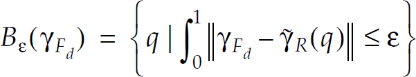
The condition defining $B_{\epsilon }({\gamma }_{F_d})$ can be replaced by the simpler condition $\parallel q_i-Q(q_i,{\gamma }_{F_d})\parallel \le {\epsilon }^{\mathrm{\prime }}(Q(q_i,{\gamma }_{F_d})$ denotes the closest point on ${\gamma }_{F_d}$ to q_i, for every i, which is equivalent to |F(q_i) – F_d| < εʺ. This last condition corresponds to what we can actually achieve as no information about ${\gamma }_{F_d}$ is available. Such a control should try to minimize the energy functional

$$\begin{array}{rl}& E_O(q(t))={\sum }_{i=0}^{N-1}(F(q_i(t))-F_d{)}^2\\ & +{\sum }_{i=1}^{N-2}(\text{acos}({\phi }_i(t))-\pi {)}^2+{\sum }_{i=0}^{N-1}({\lambda }_i(t)-d{)}^2\end{array}$$

(16) where $d=(d_1+d_2)/2,{\lambda }_i(t)=\parallel q_i(t)-q_{i-1}(t)\parallel$ , and ${\phi }_i(t)=\mathrm{\angle }((q_{i+1}-q_i)\cdot (q_{i-1}-q_i))$ . This implies that, in the absence of external tangential and normal forces, respectively, the curvature at each node should converge to zero and the robots be exactly d units apart. External normal forces are, in this simplified setting, the gradient forces. External tangential forces, on the other hand, could for instance be exerted by obstacles.

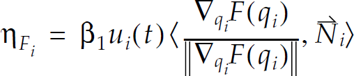
In (Kalantar, S., Zimmer, U., 2006b), we proposed a distributed control strategy for an open contour with fixed end points. In this paper, we will extend it to the case of moving end robots. First, consider the motion of interior robots. We state the equations governing the motion and refer to (Kalantar, S., Zimmer, U., 2006b) for details. Define, for i = 1, …, N − 2,

$${\dot{q}}_i(t)=v_N{\varphi }_B({\alpha }_N{\eta }_{N_i}){\stackrel{\rightharpoonup }{N}}_i+v_T{\varphi }_B({\alpha }_T{\eta }_{T_i}){\stackrel{\rightharpoonup }{T}}_i$$

(17) where ${\eta }_{N_i}(t)=({\zeta }_i{\chi }_{F_i}{\eta }_{F_i}+{\chi }_{{\kappa }_i}){\varsigma }_i$ and ${\eta }_{T_i}(t)={\chi }_{T_i}{\varsigma }_{T_i}{\eta }_{v_i}$

The symbols are explained as follows:

${\eta }_{F_i}$ is an external force (disturbance) given by

$${\eta }_{F_i}={\beta }_1{\mu }_i(t)⟨\frac{{\mathrm{\nabla }}_{q_i}F(q_i)}{\parallel {\mathrm{\nabla }}_{q_i}F(q_i)\parallel },{\stackrel{\rightharpoonup }{N}}_i⟩$$

(18) u_i(t) determines the way convergence to the isoline is to be done and a good choice for it is

$$u_i(t)=-\frac{(F(q_i)-F_d)}{{\sigma }^2}{g}_i(t)$$

(19) where $g_i(t)=G_{\sigma }(F(q_i)-F_d),G_{\sigma }(x)=1-N(0,\sigma )$ .

${\eta }_{{\kappa }_i}$ is the internal restoring force given by ${\eta }_{{\kappa }_i}={\beta }_2{v}_i(t)$ where ν _i (t) = κ _i (t)g_i(t)

${\eta }_{v_i}$ is a tangential force for uniformly distributing the robots. For the tangential motion, we put ${\eta }_{v_i}={\beta }_3{w}_i(t)$ where w_i(t) is a decreasing function of the error between the left and right energies, i.e., w_i(t) = ( e _{i, i+1} – e _{i, i−1})H^s( e _i , σ) where e _i = E_{i, i+1}(t) – E_{i, i−1}(t) is the energy difference. The energy is defined as E_{i, iω1}(t) = (1/2)e_{i, iω1}² where ω ∊ {-, +}, and e_{i, iω1} = || q_iω1, – q_i|| – d.

Finally, $H^s(x,\sigma )=1-e^{-\parallel x{\parallel }^2/{\sigma }^2}$

φ _B is a bounding function (such as tanh(αx)).

ν_N and ν_T are nominal maximum speeds for normal and tangential motions, respectively.

α _N and α _T determine the slope of the bounding function.

${\chi }_{F_i}={\chi }_{F_i^{+}}{\chi }_{F_i^{-}}$ restricts the external force to satisfy inter-robot distance constraint, where

$${\chi }_{F_i^{\omega }}=Z_{[d_1,d_2],{\epsilon }_d,\epsilon }(\parallel q_{i\omega 1}-q_i\parallel ,{\eta }_{F_i}{\stackrel{\rightharpoonup }{N}}_i,(q_{i\omega 1}-q_i))$$

(20)

Denoting Ω = [q₁, q₂], the function $Z_{\mathrm{\Omega },{\epsilon }_q,\epsilon }$ is defined by

$$Z_{\mathrm{\Omega },{\epsilon }_q,\epsilon }(q,\eta \stackrel{\rightharpoonup }{u},\stackrel{\rightharpoonup }{v})=(1-u(\tilde{\eta }))+u(\tilde{\eta })V_{\mathrm{\Omega },{\epsilon }_q,\epsilon }(q)$$

(21) where $\tilde{\eta }=W_{\mathrm{\Omega }}(q)\eta ⟨\stackrel{\rightharpoonup }{u},\stackrel{\rightharpoonup }{v}⟩$ and

$$V_{\mathrm{\Omega },{\epsilon }_q,\epsilon }(q)=1-\frac{1}{1+e^{-4\sigma Q}}$$

(22)

W_Ω(q) is zero when q ∊ Ω., is −1 when q ≥ q₂, and is equal to 1 when q ≤ q₁.

${\chi }_{{\kappa }_i}={\chi }_{{\kappa }_i^{+}}{\chi }_{{\kappa }_i^{-}}$ restricts the internal force, where

$${\chi }_{{\kappa }_i^{\omega }}=Z_{[d_1,d_2],{\epsilon }_d,\epsilon }(\parallel q_{i\omega 1}-q_i\parallel ,{\eta }_{{\kappa }_i}{\stackrel{\rightharpoonup }{N}}_i,(q_{i\omega 1}-q_i))$$

(23)

${\chi }_{T_i}={\chi }_{T_i^{+}}{\chi }_{T_i^{-}}$ constrains the tangential motion, where

$${\chi }_{T_i^{\omega }}=Z_{[d_1,d_2],{\epsilon }_d,\epsilon }(\parallel q_{i\omega 1}-q_i\parallel ,{\eta }_{v_i}{\stackrel{\rightharpoonup }{T}}_i,(q_{i\omega 1}-q_i))$$

(24)

ζ _i balances the external and internal forces to satisfy the smoothness constraint and is given by ζ _i = ζ⁰ _i ζ⁻ _i ζ⁺ _i where ${{\zeta }^0}_i=Z_{[-{\kappa }_M,{\kappa }_M],{\epsilon }_{\kappa },\epsilon }({\kappa }_i,{\eta }_{F_i}{\stackrel{\rightharpoonup }{N}}_i,{\stackrel{\rightharpoonup }{N}}_i)$ and ${{\zeta }^{\omega }}_i=V_{[-{\kappa }_M,{\kappa }_M],{\epsilon }_{\kappa },\epsilon }({\kappa }_{i\omega 1})$

${\varsigma }_{T_i}={\varsigma }_{T_i^{+}}{\varsigma }_{T_i^{-}}$ prevents any tangential motion which increases the curvature at the two neighboring robots

$${\varsigma }_{T_i^{\omega }}=Z_{-{\kappa }_M^{\mathrm{\prime }},{\kappa }_M^{\mathrm{\prime }}],{\epsilon }_{\kappa },\epsilon }({\kappa }_{i\omega 1},{\eta }_{v_i}{\stackrel{\rightharpoonup }{T}}_i-(q_i-q_{i\omega 1}{)}^{\perp })$$

(25)

ς _i is a decreasing function of e_i and is used to dampen the normal motion when the energy difference is high, thus giving tangential motion more priority. Refer to figure 3 for the visual demonstration of various forces and gains.

Fig. 3:

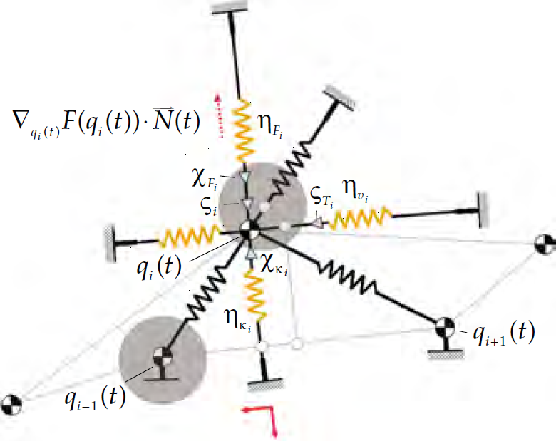
Acting forces and control terms

In this paper, to better study the behaviour of an isolated formation, we will focus on internal forces and ignore external forces which may give rise to anomalous situations. In the next section, appropriate motions for the end robots are explored.

4. Open Contours

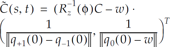
In the mathematical treatment of curve evolution by curvature, the two end points are kept fixed to symmetrize and periodize the curve. The steady state of the evolution process can then be proved to be a straight line segment (Caselles, V., Kimmel, R., Sapiro, G., 1997). In this section, we will examine various candidate motions for the end robots and will pick the most appropriate one. Consider the simplest case of a three-robot formation with just one interior robot, shown in figure 4. Let the curve Ċ(s, 0), composed of the two links connecting q₋₁(0) and q₊₁(0) to q₀(0), be evolved according to the law

$$\dot{C}(s,t)=\kappa (s,t{)}^{\lambda }{\stackrel{\rightharpoonup }{N}}_i(s,t)$$

(26)

Fig. 4:

Three-robot system

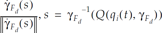
The transformed and scaled curve

$$\begin{array}{rl}& \tilde{C}(s,t)=(R_z^{-1}(\varphi )C-w).\\ & {(\frac{1}{\parallel q_{+1}(0)-q_{-1}(0)\parallel },\frac{1}{\parallel q_0(0)-w\parallel })}^T\end{array}$$

(27) will also go through the same motion. $\tilde{C}(s,0)$ can be regarded as the graph of the function $u(x,0):[-1,1]\to \mathrm{\Re }$ defined by u(x, 0) = 1 – |x|. The evolution of u would thus be

$$\frac{\mathrm{\partial }u(x,t)}{\mathrm{\partial }t}=\sqrt{1+u_x^2}{\left(\frac{u_{xx}}{(1+u_x^2{)}^{3/2}}\right)}^{\lambda }$$

(28) in (−1, 1), where u_x = ∂u/∂x and u_xx = ∂²/∂x², while u(−1, t) = u(1, t) = 0. Under these settings, convergence properties for u (and thus C) can be rigorously proved.

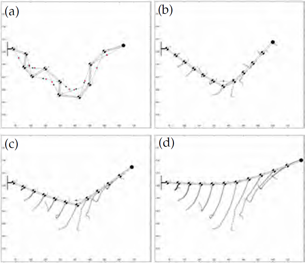
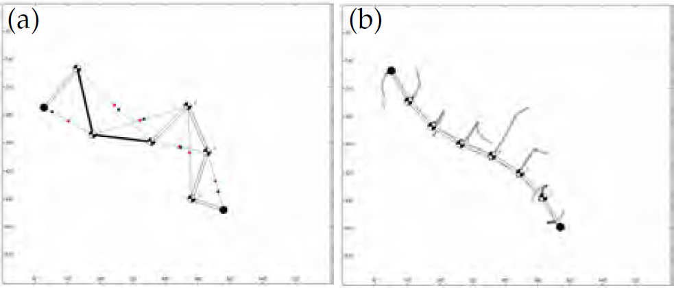
1. Figure 5(a) shows the motion of the robots following the evolution of u. q₀(t) is attached to C(1/2, t). q₋₁(t) and q₊₁(t) move in such a way that their link with q₀(t) pass through q₋₁(0) and q₊₁(0), respectively. Thus

   $$q_i(t)=\parallel q_i(0)-q_0(0)\parallel \frac{q_i(0)-q_0(t)}{\parallel q_i(0)-q_0(t)\parallel }$$
   (29) where i = −1, +1, and
   $$q_0(t)=R_z(\varphi )u(0,t)\parallel q_0(0)-w\parallel (\genfrac{}{}{0ex}{}{0}{1})+w$$
   (30) where u(0, t) is the solution of equation (28) at x = 0. As can be seen from the figure, q₋₁ and q₊₁ go through a path with considerable curvature. The tangent to the path taken by them starts from being nearly equal to (q_i – q₀)/||q_i – q₀|| to ((q_i – q₀)/||q_i – q₀||)┴ at the end of the path when the curvature at q₀ becomes zero. Also, keeping the initial start point fixed is not practical.

2. Figure 5(b) shows a situation where the motion of the two end robots is in the direction of (q_i – q₀)/||q_i – q₀|| and there are no fixed points. In this case, the line the robots converge to is shifted down considerably as a function of the initial curvature.

3. In figure 5(c), the direction of motion is (q₊₁ – q₋₁)/||q₊₁ – q₋₁||, and thus the normals at each end robot are defined to be the same as the middle robot. Although the paths of the end robots are minimal, they need to know the positions of each other and the way the normal direction is defined is, in principle, at odds with inter-robot distance constraints.

4. Figure 5(d) is a variant of that in figure 5(b), where the end robots apply a moment proportional to minus the speed function for q₀ in the direction ((q_i – q₀)/||q_i – q₀||)^⊥. This seems to be an appropriate motion in the absence of external forces. Note that, for low curvatures, the behaviour of these four strategies are basically the same.

Fig. 5:

Motions for end robots

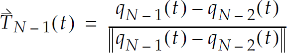
Based on these observations, we define the tangents at the two end robots of a general contour formation by

$${\stackrel{\rightharpoonup }{T}}_0(t)=\frac{q_1(t)-q_0(t)}{\parallel q_1(t)-q_0(t)\parallel }$$

(31)

$${\stackrel{\rightharpoonup }{T}}_{N-1}(t)=\frac{q_{N-1}(t)-q_{N-2}(t)}{\parallel q_{N-1}(t)-q_{N-2}(t)\parallel }$$

(32)

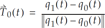
We will also artificially define

$${\kappa }_0(t)=-{\kappa }_1(t),{\kappa }_{N-1}(t)=-{\kappa }_{N-2}(t)$$

(33)

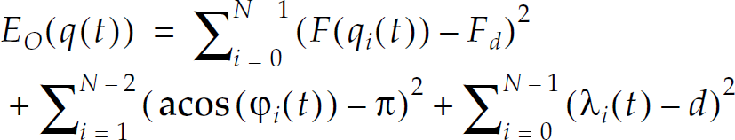
The energy errors would be

$$e_0=E_{0,1}(t),e_{N-1}(t)=-E_{N-1,N-2}(t)$$

(34) and e _{N−1, N} = e_{−1, 0} = 0. There is no need to constrain the normal motion of the end robots for satisfying inter-robot distances as, in this case, the normal direction is orthogonal to the q₁ – q₀ (respectively, q_N−1 – q_N–2) and so we define

$${\chi }_{F_0}={\chi }_{F_{N-1}}={\chi }_{{\kappa }_0}={\chi }_{{\kappa }_{N-1}}=1$$

(35)

The same is true about the tangential motion of the end robots and the constraint related to the curvature of the neighboring robots and thus ${\varsigma }_{T_0}={\varsigma }_{T_{N-1}}=1$ . Finally, define ${\chi }_{T_0^{-}}={\chi }_{T_{N-1}^{+}}=1$ and

$${{\zeta }^{+}}_{N-2}={{\zeta }^{-}}_1={{\zeta }^{+}}_{N-1}={{\zeta }^{-}}_0=0$$

(36)

ς₀ and ς_N−1 remain unchanged. See figure 6 for forces acting on an end robot.

Fig. 6:

Forces acting on end robots

5. Simulation results

Some example simulation runs are given here to demonstrate the behaviour of the discussed elastic model.

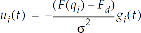
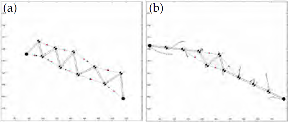
Figure 7 shows the evolution of a contour formation, fixed at one end (R₀), with no pressure from the environment, i.e., we have set ▽_qF(q) = 0 (or, more accurately, u_i(t) = 0 and g_i(t) = 0). The final configuration is a straight line. The constraints are d₁ = 60, d₂ = 120, and κ _M = 0.01. Moreover, ε _κ = 0.03 − 0.01 and ε _d = 0.1d₁. Also, β₁ = 10⁸, β₂ = 10⁴, and β₃ = 10. Figure 8 shows the evolution of a longer formation and with more initial energy. Since only one end is moving, the transmission of tangential energy dissipating pulses takes time. In this run, we have increased β₃ to 10⁵. Black lines in the snapshots indicate that the corresponding distance constraint has been violated. Similarly, darker triangles (formed by vertices q_i, q_i−1, and q_i+1) indicate higher curvatures.

Figure 9 shows the converging of a formation, with both end robots moving, to a straight line.

In figure 10, the formation stops moving before dissipating the internal energy. This is because the moving end robot (R_N−1) is constrained to remain with the framed area. Any movement of the interior robots will violate some of the constraints.

It is possible to have a formation with desired shapes. To do this, we need to designate desired curvatures for individual robots. Note that any shape can be uniquely determined by its local curvature. This can be achieved by defining $v_i(t)={\kappa }_i(t)-{\kappa }_{d_i}$ .

For example, letting ${\kappa }_{d_i}=0.01$ (for i = 0, …, N − 1), will result in an arch, as shown in figure 11. Similarly, let ${\kappa }_{d_i}=0.01$ , for $i=0,\dots ,\lceil N/2\rceil -1$ , and ${\kappa }_{d_i}=-0.01$ , for $i=\lceil N/2\rceil ,\dots ,N-1$ , to get the formation shown in figure 12. Note that, for this operation to be stable, the end points have to be kept fixed.

Figure 13 shows the motion towards and subsequent adaptation to an external profile represented by the curve ${\gamma }_{F_d}$ . Here, we use the formula

$$\frac{q_i(t)-Q(q_i(t),{\gamma }_{F_d})}{\parallel q_i(t)-Q(q_i(t),{\gamma }_{F_d})\parallel }$$

(37) for $({\mathrm{\nabla }}_{q_i}F(q_i))/\parallel {\mathrm{\nabla }}_{q_i}F(q_i)\parallel$ , where $Q(q_i(t),{\gamma }_{F_d})$ denotes the closest point on ${\gamma }_{F_d}$ to q_i(t). Also, in place of F(q_i) – F_d, we use $q_i(t)-Q(q_i(t),{\gamma }_{F_d})$ . Figure 14 shows another example.

An adapted formation can slide along the tangent to the boundary using ${\eta }_{v_i}(t)={\beta }_3{w}_i(t)+{\beta }_4{c}_T$ where c_T is a constant speed of traversal. For proper motion, we have to set c_T = 0 whenever w_i(t)c_T < 0, i.e., when they have different directions, thus giving w_i(t) higher precedence. Figure 15 shows this behaviour. Note that the robots move along the local tangent to the contour, i.e. ${\stackrel{\rightharpoonup }{T}}_i(t)$ , and not

$$\frac{{\dot{\gamma }}_{F_d}(s)}{\parallel {\dot{\gamma }}_{F_d}(s)\parallel },s={{\gamma }_{F_d}}^{-1}(Q(q_i(t),{\gamma }_{F_d}))$$

(38) assuming that the formation is sufficiently close to ${\gamma }_{F_d}$ . Normal motion will drag the robots to the boundary.

Fig. 7:

Simulation 1

Fig. 8:

Simulation 2

Fig. 9:

Simulation 3

Fig. 10:

Simulation 4

Fig. 11:

Simulation 5

Fig. 12:

Simulation 6

Fig. 13:

Simulation 7

Fig. 14:

Simulation 8

Fig. 15:

Simulation 9

6. Conclusions and future research

We defined appropriate boundary conditions for free moving open contours of robotic vehicles in the plane. The designed motion is consistent with motion of interior robots and respects the constrains imposed. This was put into the context of adaptation of these chain like formations to iso-clines or boundaries of environmental advection-diffusion processes. We have assumed no a-priori information about the process. The gradient of such field, though, should be measurable by each individual vehicle. Among the topics addressed in sequel papers are extensions to the case of non-holonomic vehicles with considerable dynamics, as well as motion constrained to manifolds, rigorous results for stability and convergence, interaction with humans, gradient estimation by groups of robots, implementation on real robots, methods for dealing with the effect of turbulence, and obstacle avoidance.