A Stable Formation Control Using Approximation of Translational and Angular Accelerations

Abstract

In this paper, a stable leader-following formation control for multiple non-holonomic mobile robot systems using only limited on-board sensor information is proposed. The control can be used for the conventional single leader – single follower (SLSF) or for novel two leaders – single follower (TLSF) schemes. The control algorithm utilizes estimations of the leaders' translational and angular accelerations in a simple form to reduce the measurement of indirect information. Simulation results show that the TLSF scheme can suppress the oscillation and damping in formation of large robot teams.

1. Introduction

In recent years, control and coordination of multi-agent systems has emerged as a topic of major interest (Liu, B.; Chu, T.; Wang, L.; & Xie, G., 2008). This is partly due to broad applications of multi-agent systems in cooperative control of unmanned vehicles, formation control of swarms, where collective motions may emerge from groups of simple individuals through limited interactions. Many swarm systems, such as flying wild geese, fighting soldiers, and robots performing a task, always form and maintain a certain kind of formation according to overlapping information structure constraints (Xu, W.B. & Chen, X.B., 2008). In practice, forming and maintaining desired formations would have great benefits for the system to perceive unknown or partially known environment, to perform its tasks. In the formation control design of mobile robots, there are various control approaches such as the behaviour-based method (Lawton, J. R. T.; Beard, R. W. & Young, B. J., 2003; Monteiro, S. & Bicho, E., 2002; Reynolds, C. W., 1987), the leader-follower method (Das, A. K., et al., 2002; Gustavi, T. & Hu, X., 2008; Wang, P. K. C., 1991), the artificial potential field method (Barnes, L.E.; Fields, M.A. & Valavanis, K.P., 2009; Wang, J.; Wu, X. & Xu, Z., 2008), the bio-inspiration method (Tanner, H. G.; Jadbabaie, A. & Pappas, G. J., 2005; Warburton, K. & Lazarus, J., 1991), the virtual-structure method (Egerstedt, M.; Hu, X. & Stotsky, A., 2001; Lewis, M. A. & Tan, K. H., 1997), the graph-based method (Desai, J. P., 2002; Fierro, R. & Das, A. K., 2002), and swarm intelligence (Gerasimos, G. R., 2008; Kwok, N. M.; Ha, Q. P. & Fang, G., 2007). Among these, due to its wide domain of application and easiness to understand and implement, the leader-follower formation control problem has received special attention and has stimulated a great deal of research. In a robot formation with leader-follower configuration, one or more robots are selected as leaders, and track predefined trajectories while the other robots, named followers, track transformed versions of the states of their leaders according to given schemes.

From the leader-following formation control strategy based on a unicycle model discussed in (Das, A. K., et al., 2002), many other papers, for instance (Kang, W.; Xi, N.; Zhao, Y.; Tan, J. & Wang, Y., 2004; Tanner, H. G.; Pappas, G. J. & Kumar, V., 2004; Vidal, R.; Shakernia, O. & Sastry, S., 2003), have also treated formation control of multiple mobile robots with unicycle dynamics. A different approach, relying on the neighbourhood-based control algorithm, has been used for the formation control law in (Jadbabaie, A.; Lin, J. & Morse, A. S., 2003; Olfati-Saber, R. & Murray, R. M., 2002), and many papers that have followed them; however, this control scheme applies to linear systems only. Other researchers have proposed the use of a second-order model of the robot for SLSF scheme and used feedback, robust and adaptive control methods (Liu, S.C.; Tan, D.L. & Liu, G.J., 2007) which analyze the acceleration of the robot in detail, even if the leader has complex trajectories (straight paths, curved paths, circular paths) but the relative orientation between the follower robot and its leader robot cannot be converged to zero.

One of the latest researches is artificial force based approach (Samitha, W. E. & Pubudu N. P., 2010) has many potential real-world applications, but the assumption that agents/members have identical physical properties limits the application of this method.

Other recent researches, such as (Sun, D.; Wang C.; Shang W. & Feng G., 2009; Wang, C. & Sun, D., 2008), transfers the formation problem to a synchronization control problem, and a synchronous controller is developed to converge both the position and synchronization (formation) errors toward zero in formation switching tasks, but they used a centralized cooperative control scheme which is susceptible to bandwidth limitation as well as external disturbances and hence is not scalable for a team with a large number of mobile agents. The drawback of complexity and resource assumption in aforementioned research is also the disadvantage of using neural networks as in (Chen, X. & Li, Y., 2008).

Besides complexity of controller, another problem is that the majority of these existing results require the measurement of the leader's speed as input to the feedback controller. The reason is that the absolute velocity of the leader cannot be measured directly by local sensors carried by the follower robot and it must be estimated by positioning measurements, which tend to enhance measurement noise dramatically; therefore, the estimation of absolute speed is difficult to obtain because it is required simultaneously in all the robot's own speed controllers. The above problems motivate the contribution of this paper.

A novel approach to this problem has recently been developed by (Gustavi, T. & Hu, X., 2008), which presents dynamic feedback controllers that do not require direct measurement of the leader's speed, but instead a method to predict that speed. However, their scheme of SLSF, which theoretically does not depend on the number of robots, is still not scalable for a big group of robots due to the accumulated errors and resulting oscillations.

This paper proposes a new stable leader-follower formation control algorithm for multiple non-holonomic mobile robots systems, which utilizes both translational acceleration and angular acceleration to control the damping/oscillations and eliminates the need to measure the leader's velocity. In addition, the control law can be quickly calculated with some basic operations and uses only some information such as distances and angles, which are easily acquired by on-board sensors. A novel TLSF scheme is also proposed to take advantage of the conventional SLSF scheme in order to deal with the unwanted oscillations and the convergence rate of all followers except the first one. The algorithm is common to both SLSF and TLSF schemes so that global formation of the local control laws can be formed flexibly and stably. It is proven that all errors in the relative states will converge to zero quickly, and the TLSF formation can have a higher rate of convergence.

This paper is organized as follows. Section 2 gives the mathematical background of the problems studied and Section 3 presents the new proposed method along with an examination of its stability and parameter tuning methodology. Section 4 will have some simulation results which show the merits of the proposed control law and this is followed by a summary and conclusions which are provided in Section 5.

2. Problem Statement

2.1. Formation

We consider a group of non-holonomic mobile robots move along a desired trajectory while maintaining a desired formation. In any case and at any time, the group of robots must do two basic tasks: forming and maintaining. Fig. 1 illustrates an example where a robot team moves along a road with a requirement to maintain a pyramid formation when the road is wide enough and a sequential formation when the road is narrow. The formation is, therefore, required to switch back and forth between the two configurations. With the leader-follower formation strategy, there is defined a group leader R0 which leads the group bulk motion, and the other robots, labelled as R _i (i = 1, 2, … n) are the followers that maintain the respective relationships with the group leader R₀, in general. However, when the number of robots in the group is large, the relationships of some followers with R₀ are hard to define due to the limitation of sensors' working range. Therefore, the definition of whole group relationships is a combination of unit relationships. Each unit contains one follower and one leader (SLSF) or two leaders (TLSF). The leaders here are local leaders, which are the robots physically close to the follower for easy sensorial connection. Hence, all robots in the group are linked, either directly or indirectly. Without loss of generality, we assume that the desired formation configurations are designed in a feasible way such that the robots can form the required formations without conflicts with each other.

Figure 1.

Motion and formation process of a group of robots with two basic tasks: forming and maintaining

This paper focuses on the formation task control only and is neither going into the details of the formation protocols for coordinating and organizing the grouped robots to accomplish the formation task, nor collision avoidance. The environment is also assumed to be obstacle free. The problem to be investigated is formulated as follows: a group of n non-holonomic mobile robots are controlled to follow a group leader R₀, which moves along a desired trajectory, and to maintain a desired form implicitly defined by the relative distance and angle between each follower and its leader (in the SLSF scheme) or the relative distances between a follower and its two leaders, as well as the relative angle with one of those two leaders (in the TLSF scheme). The SLSF and TLSF schemes are shown in Fig. 2.

Figure 2.

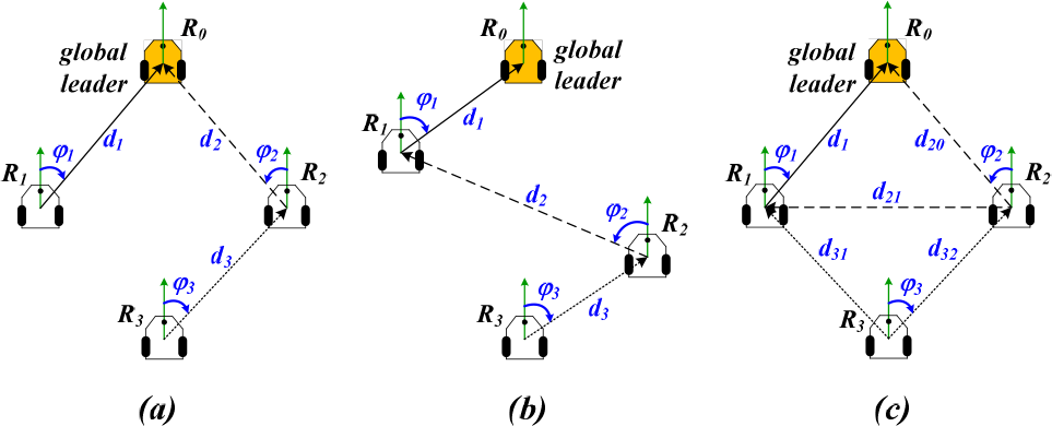
(a) SLSF scheme in diamond formation, (b) SLSF scheme in zigzag formation, and (c) TLSF scheme in diamond formation of a four-robot team.

In Fig. 2, the robot R _i (i = 1, 2, 3) must keep a relative distance d _i and a relative bearing angle φ _i with its leader in SLSF scheme. Robot R₂ and R₃ can have many choices of its leader, e.g. the leader of R₂ is R₀ in Fig. 2(a) while its leader in Fig. 2(b) is R₁. In TLSF scheme, the follower R₂ is required to follow two leaders at a distance of d₂₀ and d₂₁, respectively, as well as a bearing angle φ₂ with one of them. By changing required relative distances and a relative bearing angles, it is easily to switch from diamond form to zigzag form and vice versa.

2.2. Robot Model

This section considers a system of n non-holonomic mobile robots labelled as R₀,…, R_n-1, where R₀ is the global leader. The problem of this study deals with wheeled mobile robots with two degrees of freedom and the dynamics of the ith robot are described by the unicycle model, as follows:

$\left[\begin{array}{c}{\stackrel{.}{x}}_i\\ {\stackrel{.}{y}}_i\\ {\stackrel{.}{\theta }}_i\end{array}\right]=\left[\begin{array}{cc}\cos {\theta }_i& 0\\ \sin {\theta }_i& 0\\ 0& 1\end{array}\right]\left[\begin{array}{c}{v}_i\\ {\omega }_i\end{array}\right]$

(1)

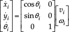
where v _i is the linear velocity, ω _i is the angular velocity of the mobile robot, θ _i is the angle between the heading direction and the x axis, and (x _i ,y _i ) are the Cartesian coordinates of the centre of mass of the vehicle (see Fig. 3).

Figure 3.

SLSF scheme

2.3. Formation Control Framework for SLSF scheme

In SLSF configuration (shown in Fig. 3), R _i is leader robot and R _k is follower robot. Let d _ki denote the actual distance between R _i and R _k , φ _ki is the actual bearing angle from the orientation of R _k to the d _ki -axis (the axis connecting R _i and R _k ). The definition of the SLSF formation scheme requires that distance between R _i and R _k to be equal to d _k0 and the bearing angle from the orientation of R _k to the d _ki -axis is desired to be φ _k0 .

The difference between headings of two robots is defined as:

$\mathrm{\Delta }{\theta }_k={\theta }_k-{\theta }_i$

(2)

Based on the configuration and these definitions, the dynamics of the system are expressed as:

${\stackrel{.}{d}}_{ki}=-v_k\cos {\phi }_{ki}+v_i\cos \left({\phi }_{ki}+\mathrm{\Delta }{\theta }_k\right)$

(3)

${\stackrel{.}{\phi }}_{ki}=-{\omega }_k+v_k\frac{\sin {\phi }_{ki}}{d_{ki}}-v_i\frac{\sin \left({\phi }_{ki}+\mathrm{\Delta }{\theta }_k\right)}{d_{ki}}$

(4)

$\mathrm{\Delta }{\stackrel{.}{\theta }}_k={\omega }_k-{\omega }_i$

(5)

where (5) can be derived easily from (2) by taking the derivative of both sides. Equation (3) is found from the observation that on d _ki -axis, the change of relative distance between two robots (d _ki ) is the difference in the velocities of R _i and R _k . To derive equation (4), note that the change of bearing angle (φ̇ _ki ) is caused by three components: the angular velocity of R _k , the relative motion of R _i to R _k , and the relative motion of R _k to R _i . The objective of the leader–follower control in SLSF scheme, therefore, is stated as following:

Control objective 1: Given v _i (t) and ω _i (t), find control v _k (t) and ω _k (t) for SLSF scheme such that

$\begin{array}{l}{d}_{ki}\to d_{k0},{\phi }_{ki}\to {\phi }_{k0},\mathrm{\Delta }{\theta }_k\to 0\text{\hspace{0.17em}\hspace{0.17em}as\hspace{0.17em}\hspace{0.17em}\hspace{0.17em}\hspace{0.17em}}t\to \infty ,\\ i=\overline{0,n-1},k=\overline{1,n}\text{\hspace{0.17em},\hspace{0.17em}\hspace{0.17em}\hspace{0.17em}\hspace{0.17em}}\left|{\phi }_{k0}\right|\le \frac{\pi }{2}.\end{array}$

(6)

In order to solve this problem, a reference point M(x _km , y _km ) is chosen (see Fig. 3) at a distance d _k0 from the leader in the direction whose angular deviation with the orientation of the follower robot is φ _k0 . Hence, the coordinates of reference point can be calculated by:

$\left[\begin{array}{c}{x}_{km}\\ y_{km}\end{array}\right]=\left[\begin{array}{c}{x}_i\\ y_i\end{array}\right]+\left[\begin{array}{c}-\cos \left({\theta }_k+{\phi }_{k0}\right)\\ -\sin \left({\theta }_k+{\phi }_{k0}\right)\end{array}\right]d_{k0}$

(7)

With the definition of this reference point, the desired control of the follower robot can be obtained by controlling the position of follower (x _k , y _k ) towards (x _km , y _km ). This means that the distance d _ki and the angle of orientation, φ _ki , can be simultaneously controlled so that the relative distance d _ki and relative bearing angle φ _ki approaches d _k0 and φ _k0 respectively.

3. Proposed Control

3.1. Formation Control Framework for TLSF Scheme

The system of n mobile robots is the same as SLSF scheme and the robot R _j is required to keep a distance d _j0 from its leader R _i and its bearing angle at φ _j0 . However, the robot R _k in this scheme must simultaneously follow two leaders with two desired separations to R _i and R _j of d _k0 and l _k0 , respectively, besides the desired bearing angle φ _k0 from the orientation of R _k to the d _ki -axis.

As shown in Fig. 4, the three robots are currently located at A, B, and C, and the desired formation is the triangle ΔADE (d_j0 = AE, d_k0 = AD, l _k0 = DE). The triangle ΔAMN is found by rotating the triangle ΔADE an angle Ψ so that the side AE always lies on the d _ji -axis. By this definition, the robot R _j is controlled to reach E (N comes towards E) and the robot R _k is controlled to reach M (M will come towards D because of N). When R _j is at E, R _k is obviously at D, as is required. Therefore, TLSF helps both followers reach the desired points nearly at the same time, and the oscillations in the motion of R _k on the way to reach a stable state are restricted by the constraint with the second leader R _j . This is the major difference between the two schemes. In the SLSF scheme, the second follower can be only at a stable state after the first follower is stable. However, the TLSF scheme implicitly requires that the two leaders must be well configured and controlled, or the follower may encounter difficulties.

Figure 4.

TLSF scheme

The pair R _i - R _j is the SLSF scheme, then the remaining is finding the reference point for R _k . From two required separations d _k0 and l _k0 , and desired bearing angle φ _k0 , the instantaneous bearing angle φ _km can be calculated as follows:

${\phi }_{km}=\arccos \left(\frac{x_i-x_m}{d_{k0}}\right)-{\theta }_k$

(8)

where $x_m=\frac{{\alpha }_2\pm ({\alpha }_2^2-4{\alpha }_1{\alpha }_3)}{{\alpha }_1}$ , with

${\alpha }_0=\frac{1}{2}\left[\left(x_i^2-x_n^2\right)+\left(y_i^2-y_n^2\right)-d_{k0}^2+l_{k0}^2\right]$

${\alpha }_1=2\left(\mathrm{\Delta }{x}^2+\mathrm{\Delta }{y}^2\right)$

${\alpha }_2=2\left[{\alpha }_0\mathrm{\Delta }x-\mathrm{\Delta }y\left(y_i\mathrm{\Delta }x-x_i\mathrm{\Delta }y\right)\right]$

${\alpha }_3={\left({\alpha }_0-y_i\mathrm{\Delta }y\right)}^2-{\left(x_i\mathrm{\Delta }y\right)}^2-{\left(d_{k0}\mathrm{\Delta }y\right)}^2$

$\mathrm{\Delta }x=x_i-x_n$

$\mathrm{\Delta }y=y_i-y_n$

$x_n=x_i+\frac{d_{j0}}{d_{ji}}(x_j-x_i)$

$y_n=y_i+\frac{d_{j0}}{d_{ji}}(y_j-y_i)$

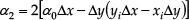
To choose the unique value of φ _km , we need to compare directions of the two vectors AN→ and AM→, as shown in Fig. 4, which are defined as

$\{\begin{array}{c}\overrightarrow{AN}=\left(\left(x_n-x_i\right),\left(y_n-y_i\right)\right)\\ \overrightarrow{AM}=\left(\left(x_m-x_i\right),\left(y_m-y_i\right)\right)\end{array}$

These give a criterion of

${\alpha }_4=(x_m-x_i)(y_n-y_i)-(x_n-x_i)(y_m-y_i)$

(9)

When M is at the left-hand side of AN→, select x _m such that α₄ > 0, and vice versa.

The objective of the leader–follower control in TLSF scheme is re-stated from SLSF scheme as following:

Control objective 2: Given v _i (t) and ω _i (t), find control v _k (t) and ω _k (t) for TLSF scheme such that

$\begin{array}{l}{d}_{ki}\to d_{k0},\hspace{0.17em}{\phi }_{ki}\to {\phi }_{km},\hspace{0.17em}\mathrm{\Delta }{\theta }_k\to 0\text{\hspace{0.17em}\hspace{0.17em}\hspace{0.17em}as\hspace{0.17em}\hspace{0.17em}\hspace{0.17em}}t\to \infty ,\\ i=\overline{0,n-1},\hspace{0.17em}k=\overline{2,n}.\end{array}$

(10)

Compared with the SLSF scheme, the only difference is that the bearing angle in the SLSF scheme is a constant, but the bearing angle in the TLSF is not. This is an advantage in building the control rule because the control rule just needs to deal with the time-variant bearing angle φ _km then it can apply to both schemes, so that the bearing angle in the proposed control algorithm, which is presented in the next section, is time-varying.

3.2. Proposed Control Law

Fig. 5 is redrawn from Fig. 4 with some supporting information in order to find the following control: as t→∞, the follower robot's position (x _k (t),y _k (t)) can be controlled to reach the reference point (x _km (t),y _km (t)), i.e. the point C needs to approach the point M.

Figure 5.

TLSF scheme with detailed information

Now consider the d _k0 -axis. On this direction, the change of position from C to M is mirrored as the change from F to M and the component on the d _k0 -axis of the relative velocity between v _k and v _i will do this task. Therefore, the following is obtained:

$v_k\cos \left({\phi }_{km}\right)-v_i\cos \left({\phi }_{km}+\mathrm{\Delta }{\theta }_k\right)=k_1\left[d_{ki}\cos \left({\phi }_{ki}-{\phi }_{km}\right)-d_{k0}\right]$

(11)

where k₁ is a postitive tuning coefficient.

Next, in order to find ω _k , the a _k -axis should be considered, as shown in Fig. 5 to be perpendicular to v _k . Similar to the way of calculating v _k , the change of velocity on this axis (C→G) is caused by the rotation with angular velocity ω _k and v _i which gives:

$\begin{array}{c}\left({\omega }_k+{\omega }_i\right)d_{ki}\cos \left({\phi }_{km}\right)=k_1\left[d_{ki}\cos \left({\phi }_{ki}\right)-d_{k0}\sin \left({\phi }_{km}\right)\right]\\ \hspace{1em}\hspace{1em}-v_i\sin \left(\mathrm{\Delta }{\theta }_k\right)\end{array}$

(12)

One problem is that the above control rule and most other controllers in the literature require the measurement of the leader's speed v _i which is practically impossible using only onboard sensors particularly if the speed is supposed to be fed back into the robot's own speed regulation, as in equations (11) and (12). In addition, ω _i is also impossible to measure.

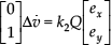
In (Gustavi, T. & Hu, X., 2008), the authors tried to estimate only v _i by mathematically transform the system model into a cascade system for easier analysis. However, they must assume that ω _i = 0 and v̇ _i = 0 to decouple the system for proving stability by Lyapunov theory. The aim of our method is to build a control law that can both compensate the change of v _i and ω _i , and drive the follower to the desired position, without knowing the exact value of v _i and ω _i , based on a kinematic analysis (Fig. 5). In order to do this, R _k should be considered in the coordinate of R _i , i.e. the coordinate (x _i , y _i ), instead of (x,y). In this coordinate, R _i is not moving and there is a velocity -v _i applied to R _k . Assuming that v _i at time t becomes v _i + Δv _i at time t + Δt which will put into the control of R _k a component Δv to adaptively compensate the change of v _i . This is the change of velocity in the time step, so it is also the instantaneous translational acceleration of leader robot, and can be approximated by:

$\begin{array}{l}{\stackrel{.}{v}}_a=k_2\mathrm{sgn}\left[\cos \left(2{\theta }_i\right)\right]\\ \hspace{1em}\hspace{0.17em}\times \left[d_{ki}\cos \left({\phi }_{ki}+\mathrm{\Delta }{\theta }_k\right)-d_{k0}\cos \left({\phi }_{km}+\mathrm{\Delta }{\theta }_k\right)\right]\end{array}$

(13)

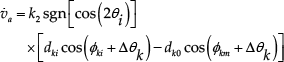
where k₂ > 0 is another tuning coefficient, and v _a = v _i + Δv. Using the same technique as applied with the leader's velocity, that is, the change Δω of ω _km is also considered from time t to time t+Δt and Δω is then the angular acceleration of the reference point and can be approximated by:

$\begin{array}{l}{\stackrel{.}{\omega }}_a=k_x\frac{e_x\left(\sin \left(\mathrm{\Delta }{\theta }_k\right)\sin {\phi }_{km}-\cos \left(\mathrm{\Delta }{\theta }_k\right)\right)}{d_{k0}\cos {\phi }_{km}}\\ \hspace{1em}\hspace{0.17em}-k_y\frac{e_y\left(\cos \left(\mathrm{\Delta }{\theta }_k+{\phi }_{km}\right)\sin {\phi }_{km}+\sin \left(\mathrm{\Delta }{\theta }_k\right)\right)}{d_{k0}\cos {\phi }_{km}}\end{array}$

(14)

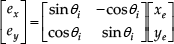
where k _x and k _y are tuning coefficients. ω _a = ω _km + Δω, e _x = -d_k0 sin(Δθ _k + φ _km ) + d _ki sin(Δθ _k + φ _ki ), and e _y = d_k0 cos(Δθ _k + φ _km ) - d _ki cos(Δθ _k + φ _ki ).

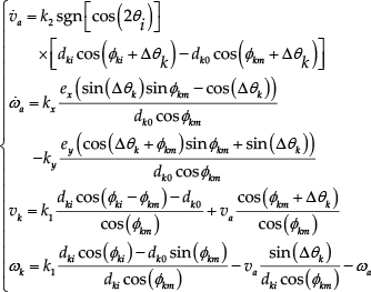
In summary, the proposed leader-follower control is equation (15). As seen in equation (15), the control law requires values of d _ki , φ _ki , Δθ _k which are assumed to be available by measurements from the on-board sensors.

$\{\begin{array}{ll}{\stackrel{.}{v}}_a\hfill & =k_{2}sgn[cos(2{\theta }_i)]\hfill \\ \hfill & \hspace{0.17em}\hspace{0.17em}\times [d_{ki}cos({\varphi }_{ki}+\Delta {\theta }_k)-d_{k0}cos({\varphi }_{km}+\Delta {\theta }_k)]\hfill \\ {\stackrel{.}{\omega }}_a\hfill & =k_x\frac{e_x(sin(\Delta {\theta }_k)sin{\varphi }_{km}-cos(\Delta {\theta }_k))}{d_{k0}cos{\varphi }_{km}}\hfill \\ \hfill & -k_y\frac{e_y(cos(\Delta {\theta }_k+{\varphi }_m)sin{\varphi }_{km}+sin(\Delta {\theta }_k))}{d_{k0}cos{\varphi }_{km}}\hfill \\ {\nu }_k\hfill & =k_1\frac{d_{ki}cos({\varphi }_{ki}-{\varphi }_{km})-d_{k0}}{cos({\varphi }_{km})}+{\nu }_a\frac{cos({\varphi }_{km}+\Delta {\theta }_k)}{cos({\varphi }_{km})}\hfill \\ {\omega }_k\hfill & =k_1\frac{d_{ki}cos({\varphi }_{ki})-d_{k0}sin({\varphi }_m)}{d_{ki}cos({\varphi }_{km})}-{\nu }_a\frac{sin(\Delta {\theta }_k)}{d_{ki}cos({\varphi }_{km})}-{\omega }_a\hfill \end{array}$

(15)

The necessary information includes only distance and angles, and many kinds of sensor can be used to gather those data. In the SLSF scheme, φ _km = φ _k0 = const. and ω _a = 0, so it is not necessary to use the second equation of (15). Our approach is based on the approximation of accelerations, which helps to build a common control law for both SLSF and TLSF schemes. Therefore, it is generally different from the control law in (Gustavi, T. & Hu, X., 2008) which can be applied to an SLSF scheme only.

Theorem : Suppose that the motion of the leader robot R _i satisfies the following condition:

v _i (t) ⩾ v₀ > 0, v̇ _a (t) ∈ L₂[0, ∞), ω _i (t) ∈ L₂[0,∞), ω̇ _a (t) ∈ L₂[0,∞). Then, with the control (15), where we let

$\{\begin{array}{l}0<k_x<k_1^2\\ -k_2\mathrm{sgn}\left[\cos \left(2{\theta }_i\right)\right]<k_y<k_1^2-k_2\mathrm{sgn}\left[\cos \left(2{\theta }_i\right)\right]\end{array}$

(16)

as t → ∞ we will have globally (x _k , y _k ) → (x _km , y _km ), i.e. d _ki → d _k0 and φ _ki → φ _km .

Proof: Let

$\left[\begin{array}{c}{x}_e\\ y_e\end{array}\right]=\left[\begin{array}{c}{x}_k\\ y_k\end{array}\right]-\left[\begin{array}{c}{x}_{km}\\ y_{km}\end{array}\right]$

(17)

and define

$\left[\begin{array}{c}{e}_x\\ e_y\end{array}\right]=\left[\begin{array}{cc}\sin {\theta }_i& -\cos {\theta }_i\\ \cos {\theta }_i& \sin {\theta }_i\end{array}\right]\left[\begin{array}{c}{x}_e\\ y_e\end{array}\right]$

(18)

Equations (3), (4) and (5) can be rewritten as

$\left[\begin{array}{c}{\stackrel{.}{e}}_x\\ {\stackrel{.}{e}}_y\end{array}\right]=-k_1\left[\begin{array}{c}{e}_x\\ e_y\end{array}\right]+\mathrm{\Delta }v\left[\begin{array}{c}0\\ 1\end{array}\right]-\mathrm{\Delta }\omega d_{k0}\left[\begin{array}{c}\cos \left(\mathrm{\Delta }{\theta }_k+{\phi }_{km}\right)\\ \sin \left(\mathrm{\Delta }{\theta }_k+{\phi }_{km}\right)\end{array}\right]$

(19)

Consider a Lyapunov function candidate as

$V={\left(e_x+\frac{{\omega }_c}{k_1}\right)}^2+{\left(e_y-\frac{\mathrm{\Delta }v}{k_1}+\frac{{\omega }_s}{k_1}\right)}^2+\frac{1}{k_1^2}{\left({\omega }_s-\mathrm{\Delta }v\right)}^2$

(20)

where ω _c = Δωd_k0 cos(Δθ _k + φ _km ), ω _s = Δωd_k0 sin[Δθ _k + φ _km ). Before examining this Lyapunov function, there are several matrices, and a number which needs to be defined:

$\gamma =\mathrm{\Delta }{\theta }_k+{\phi }_{km}$

(21)

$P=\left[\begin{array}{cc}{k}_x& 0\\ 0& k_y\end{array}\right]=P^T$

(22)

$s=\mathrm{sgn}\left[\cos \left(2{\theta }_i\right)\right]$

(23)

$G=\left[\begin{array}{cc}sin\gamma & -cos\gamma \\ cos\left(\mathrm{\Delta }{\theta }_k\right)& sin\left(\mathrm{\Delta }{\theta }_k\right)\end{array}\right]$

(24)

$\Rightarrow G^{-1}=\frac{1}{cos\left({\phi }_{km}\right)}\left[\begin{array}{cc}sin\left(\mathrm{\Delta }{\theta }_k\right)& cos\gamma \\ -cos\left(\mathrm{\Delta }{\theta }_k\right)& sin\gamma \end{array}\right]$

(25)

$Q=\left[\begin{array}{cc}0& 0\\ 0& -s\end{array}\right]$

(26)

$W=\left[\begin{array}{c}{\omega }_c\\ {\omega }_s\end{array}\right]$

(27)

The derivation of this Lyapunov function is long but not difficult, so only some of the key steps are shown here, in which the derivative of a scalar variable is denoted by a dot, while the derivative of a matrix valued function is denoted by a prime. The variable in scalar is in lower case, and the matrix is presented in capital letters (except V).

Taking derivative of V, we have

$\begin{array}{l}\frac{\stackrel{.}{V}}{2}=\left[\begin{array}{cc}{e}_x+\frac{{\omega }_c}{k_1}& e_y-\frac{\mathrm{\Delta }v}{k_1}+\frac{{\omega }_s}{k_1}\end{array}\right]{\left(\left[\begin{array}{c}{e}_x\\ e_y-\frac{\mathrm{\Delta }v}{k_1}\end{array}\right]+\left[\begin{array}{c}{\omega }_c\\ {\omega }_s\end{array}\right]\right)}^{\text{'}}\\ \hspace{1em}+\frac{1}{k_1^2}\left(-\mathrm{\Delta }v+W^T\right)\left(-\mathrm{\Delta }\stackrel{.}{v}+W^{\text{'}}\right)\end{array}$

(28)

By noting the following properties,

$\left[\begin{array}{c}0\\ 1\end{array}\right]\mathrm{\Delta }\stackrel{.}{v}=k_{2}Q\left[\begin{array}{c}{e}_x\\ e_y\end{array}\right]$

(29)

$Q\left[\begin{array}{c}0\\ 1\end{array}\right]\frac{\mathrm{\Delta }v}{k_1}=\left[\begin{array}{c}0\\ -s\end{array}\right]\frac{\mathrm{\Delta }v}{k_1}$

(30)

$Q\left[\begin{array}{c}{\omega }_c\\ {\omega }_s\end{array}\right]=0$

(31)

$W\text{'}={\left[\begin{array}{c}{\omega }_c\\ {\omega }_s\end{array}\right]}^{\text{'}}=P\left[\begin{array}{c}{e}_x\\ e_y\end{array}\right]=\left[\begin{array}{cc}{k}_x& 0\\ 0& k_y\end{array}\right]\left[\begin{array}{c}{e}_x\\ e_y\end{array}\right]\Rightarrow \{\begin{array}{c}{\stackrel{.}{\omega }}_c=k_x{e}_x\\ {\stackrel{.}{\omega }}_s=k_y{e}_y\end{array}$

(32)

$\begin{array}{r}\frac{1}{k_1^2}\left(-\mathrm{\Delta }v+W^T\right)\left(-\mathrm{\Delta }\stackrel{.}{v}+W^{\text{'}}\right)=\left[\begin{array}{cc}{e}_x& e_y\end{array}\right]\left(-\frac{k_{2}Q}{k_1}+\frac{P}{k_1}\right)\\ \hspace{0.17em}\times \left(\frac{1}{k_1}\left[\begin{array}{c}{\omega }_c\\ {\omega }_s\end{array}\right]-\left[\begin{array}{c}0\\ 1\end{array}\right]\frac{\mathrm{\Delta }v}{k_1}\right)\end{array}$

(33)

it is easily to derive

$\begin{array}{l}\frac{\stackrel{.}{V}}{2}=-\left(k_1-\frac{k_x}{k_1}\right){\left(e_x+\frac{{\omega }_c}{k_1}\right)}^2\\ \hspace{1em}\hspace{1em}-\left(k_1-s\frac{k_2}{k_1}-\frac{k_y}{k_1}\right){\left(e_y-\frac{\mathrm{\Delta }v}{k_1}+\frac{{\omega }_s}{k_1}\right)}^2\\ \hspace{1em}\hspace{1em}-\frac{k_x}{k_1^3}{\omega }_c^2-\frac{1}{k_1^2}\left(s\frac{k_2}{k_1}+\frac{k_y}{k_1}\right){\left({\omega }_s-\mathrm{\Delta }v\right)}^2\end{array}$

(34)

It is obvious that if the condition (16) is satisfied, v̇ ⩽ 0. This implies that e _x and e _y are exponentially convergent to zero. ▪

4. Simulations and Analysis

In order to show the validity, quality and feasibility of the proposed leader-follower control method, we carried out several simulations. We will compare our new control law (15) with the control law proposed in (Gustavi, T. & Hu, X., 2008) (which will be called control law [Ref] from now on). The time step is chosen at 0.2s, which assumes 0.1s for the measurement and communication, and 0.1s for the driving and transportation. The leader is controlled to follow a sinusoidal path, which is similar to (Gustavi, T. & Hu, X., 2008) for purpose of comparison, with a slowly varying speed. Besides those parameter settings, we will compare the performance of control laws in both forming and maintaining tasks in small-scale as well as large-scale robot teams.

4.1. First Simulation

A simulation with control law (15) is performed to form a line formation of the three robots, where robot R₀ is the global leader. At the beginning the three robots may be placed anywhere in the field. However for this simulation, we will specify the initial states of the three robots as [x₀, y₀, θ₀] = [0, 0, 0], [x ₁ , y ₁ , θ ₁ ] = [−1.5, −2.6, 0], and [x₂, y₂, θ₂] = [−3, −5.2, 0]. The desired distance between the follower R₁ and R₀ is 3m and the desired bearing angle is π/6. The follower R₂ is required to keep a distance of 3m and 6m to R₁ and R₀ respectively, and a bearing angle of π/6 with R₀. Another simulation using control law [Ref] is also conducted with a similar configuration and the only difference is that R₂ is not required to keep a distance of 6m with R₀.

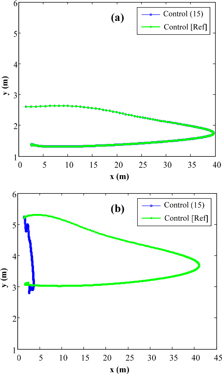
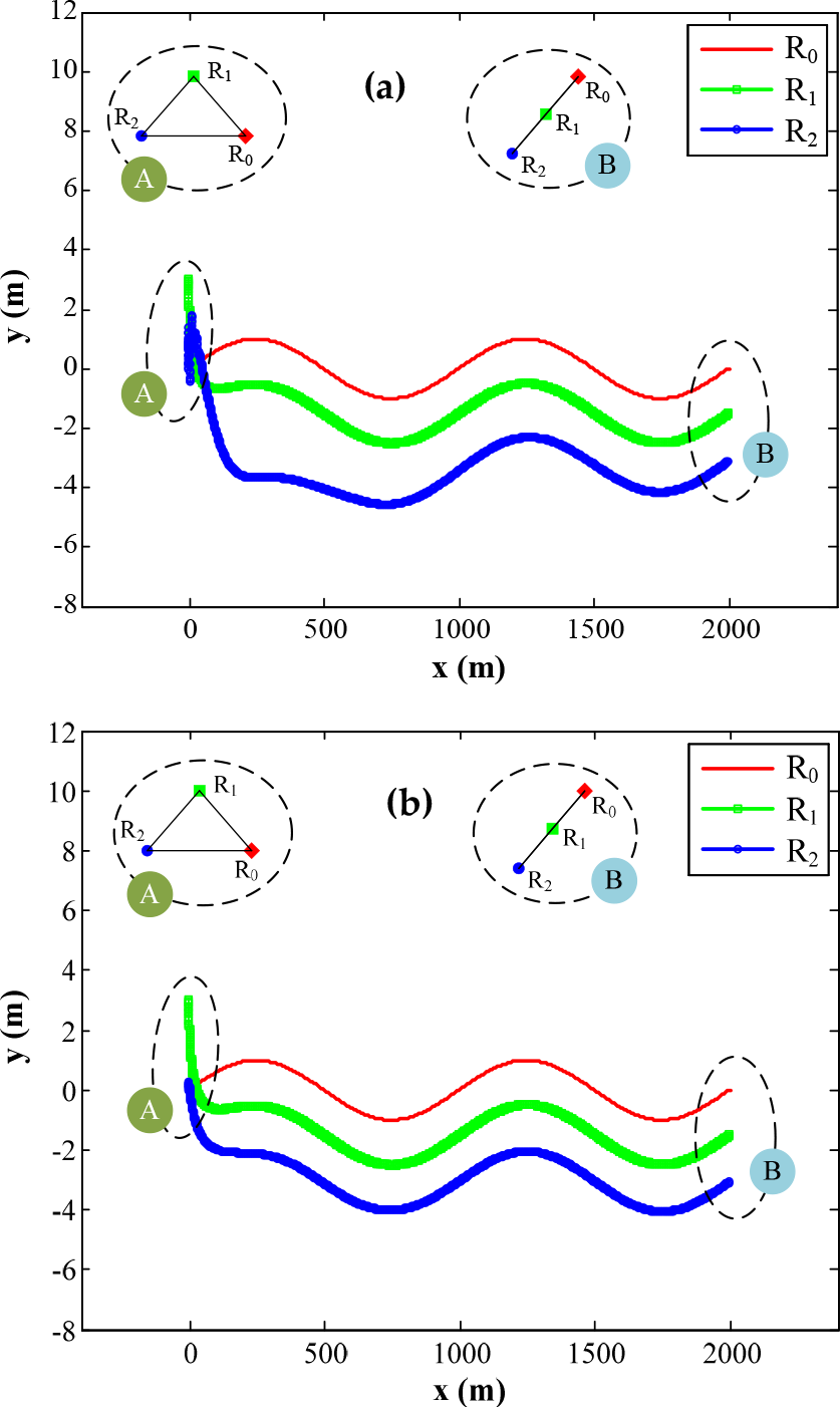
Fig. 6 shows the performance of the two control laws in the global x-y coordinates. There is only a small difference in the trajectory of robot R₂ can be seen from Figs. 6(a) and 6(b). It is not apparent that R₂ tracks the leaders better (quicker convergence) when using control law (15) than when using control law [Ref]. Figs. 7, 8 and 9 will show this more clearly. As seen from Figs. 7(a), 8(a) and 9(a), the robots' performance based on the new control law (15) is not significantly different from performance based on control law [Ref] because this is the SLSF scheme in both cases.

Figure 6.

Performance of (a) control law [Ref] and (b) control law (15).

Figure 7.

Trajectory seen from leader robot R₀ of (a) R₁ and (b) R₂.

Figure 8.

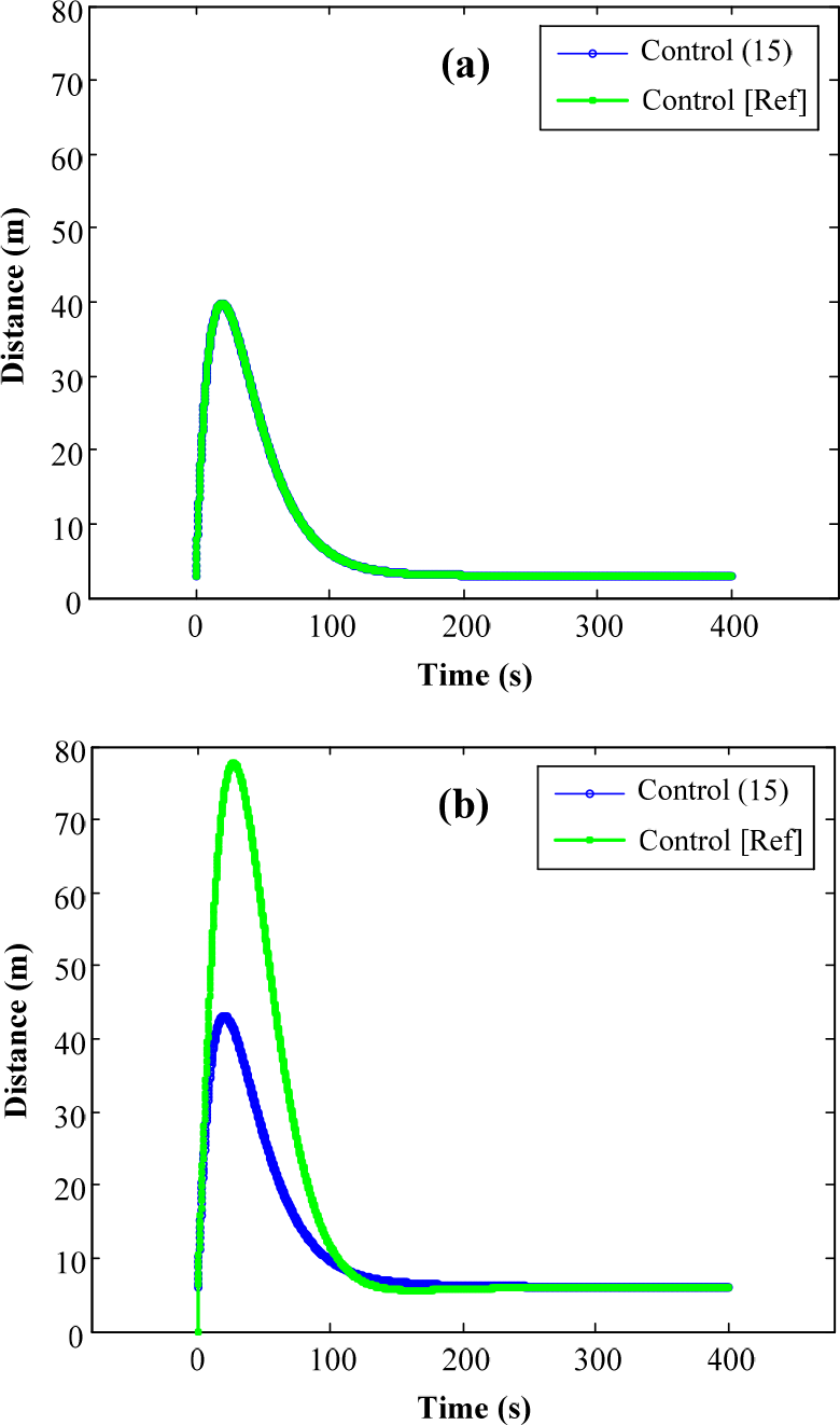
Relative distance over time between (a) R₁ and R₀ and (b) R₂ and R₀.

Figure 9.

Relative bearing angle over time between (a) R₁ and R₀, and (b) R₂ and R₀.

However, there is an advantage of the new control law (15) in the TLSF scheme, as seen in Figs. 7(b), 8(b) and 9(b). In Fig. 7(b), the robot R₂ quickly approaches the desired position with the trajectory being nearly a straight line due to the existence of the constraint about the distance with R₁, while robot R₂ using control [Ref] moves in a long curve before reaching the desired position. In Fig. 8(b), the error of R₂ in the SLSF seems to be cumulative with the error of R₁, so the farthest distance that it has with R₀ is about double. Meanwhile the TLSF scheme causes R₂ to have a similar behavior as R₁, and to converge to a stable state nearly at the same time as R₁. These are two advantages of the new controller (15) within the TLSF scheme. Fig. 9(b) shows the advantage of the approximation of the angular velocity. In the SLSF scheme, there is no constraint for the bearing angle, so oscillations easily occur.

By approximating the angular acceleration of the reference point in the new control law (15) and choosing appropriate parameters, the oscillations and damping can be reduced.

4.2. Second Simulation

The second simulation demonstrates that it is possible and beneficial to apply the algorithm to a large team of robots. The number of robots is now 5 and the trajectory of the leader is still sinusoidal and the robots form a line with the distance between each adjacent robot being 3m, and the bearing angle is π/6. The performance of the controller [Ref] and the new controller (15) are compared in Fig. 10.

Figure 10.

Performance of a team of 5 robots using (a) the control law [Ref] and (b) the control law (15) in the TLSF scheme.

From Fig. 10 and the displacement error values presented in Tables 1 and Table 2, it can be seen that the controller (15) has better performance, especially for robots which are at greater distance from the global leader. The convergence rate is faster and the transient errors are smaller. The mean and standard deviation of both distance and angular errors of the second, third and fourth follower robots using controller (15) are much less than when using controller [Ref]. Moreover, those values do not show much difference nor are they incremental as when using controller [Ref]. This means that the TLSF scheme simply keeps the errors away from cumulation.

Table 1.

Displacement errors of control law [Ref]

Follower no.	mean Λ/dk0	std Δ/dk0	mean Δφ km	std Δφ km
1	0.6539	2.2384	−0.0982	0.2514
2	0.6595	2.3966	−0.0624	0.2653
3	0.6790	2.5985	0.0429	0.5103
4	0.7543	2.8104	0.1909	0.9620

Table 2.

Displacement errors of control law (15)

Follower no.	mean Δd/dk0	std Δd/dk0	mean Δφ km	std Δφ km
1	0.6536	2.2384	−0.0982	0.2514
2	0.3229	1.1045	−0.0798	0.2139
3	0.3203	1.1910	−0.0804	0.2318
4	0.3212	1.1895	−0.0786	0.2216

4.3. Third Simulation

In above two simulations, the formation-maintaining task is shown. In third simulation, the forming task is performed. A four-robot team will change from a triangular form to a line form (Fig. 11). At first, the three robots are keeping the triangular form (form A), where R₀ is the global leader. The initial poses of R₀, R₁, and R₂ are (0, 0, 0), (−2, 2, 0), and (−2, −2, 0), respectively. The team is required to change to a line form (form B) where R₁ follows R₀ with a distance of 3m and bearing angle π/4; R₂ follows R₀ with bearing angle of π/4 and distance of 6m, and simultaneously keeps a distance 3m with R₁. The results are depicted in Fig. 11. It is shown that the formation is switched well and quickly. The trajectory of R2 when using controller (15) is not as smooth as when using controller [Ref], but the overall error is smaller. All the advantages of TLSF scheme and controller (15) stated in section 4.2 above are also shown in this simulation (see Table 3 and Table 4).

Figure 11.

Performance of a team of 3 robots in switching from a triangular formation to a line formation using (a) control law [Ref] and (b) control law (15)

Table 3.

Displacement errors of control law [Ref] in forming task

Follower no.	mean Δd/dk0	std Δd/dk0	mean Δφ km	std Δφ km
1	2.4222	4.9308	−0.2771	0.3772
2	2.4602	5.2911	−0.1560	0.4420

Table 4.

Displacement errors of control law (15) in forming task

Follower no.	mean Δd/dk0	std Δd/dk0	mean Δφ km	std Δφ km
1	2.1946	4.6062	−0.2610	0.3709
2	1.3069	2.4982	−0.2038	0.3831

5. Conclusions

In this paper, we propose a new leader-following control method for swarm formation using the approximation of translational and angular accelerations. The control law can be applied to both SLSF and TLSF schemes. Simulations have been presented which show that the stability of the control algorithm can be achieved by tuning the parameters properly, and the algorithm can work well in any scale of formation. The TLSF scheme is better for larger groups of robots because the approximation of the angular acceleration can help to suppress the damping and oscillations and increase convergence rate of the third, fourth, and succeeding follower robots. In addition, the controller uses only available data of the distances and the angles, acquired from onboard sensors. No indirect data such as the translational velocity and angular velocity of the leader robot are required. Thus the number of measurements is reduced, the errors from the measurements are smaller and as a consequence the calculation time is shorter.