
Abstract
In this article, we present a human experience–inspired path planning algorithm for service robots. In addition to considering the path distance and smoothness, we emphasize the safety of robot navigation. Specifically, we build a speed field in accordance with several human driving experiences, like slowing down or detouring at a narrow aisle, and keeping a safe distance to the obstacles. Based on this speed field, the path curvatures, path distance, and steering speed are all integrated to form an energy function, which can be efficiently solved by the A* algorithm to seek the optimal path by resorting to an admissible heuristic function estimated from the energy function. Moreover, a simple yet effective fast path smoothing algorithm is proposed so as to ease the robots steering. Several examples are presented, demonstrating the effectiveness of our human experience–inspired path planning method.
Introduction
The path planning, which refers to designing a path for navigating an agent toward a desired location from a start position, has been widely applied in robotics community and other real application fields, 1 such as window cleaning, 2 exploration of Mars, and video game. 3 Among these applications, path planning for service robots plays a central role in complex indoor and outdoor environments. 4
In general, path planning is to find a sequence of location transition actions that transform a start position to a goal position, where each transition action has an associated cost, and the sum of costs of all transition actions represents some measurement for the path. Designing transition actions for path planning generally concerns on following aspects: (i) travel time between the start position and the goal position (also referred as the time factor); (ii) energy spent of an agent traveling a path; (iii) robots do not collide with other objects; and (iv) smoothness of a path is desired to ease steering of robots. Currently, main path planning methods aim at designing an optimization model which considers one or more of the above-mentioned aspects, and then performing a minimization procedure to achieve an optimal path. 1,4 –7 For example, the shortest path, minimum time-consuming path, minimal energy cost, and coverage path planning are, respectively, studied in the literature 6,8,9 for a given navigation task. Path planning involves four developing stages: graph-based methods (e.g. Dijkstra, Voronoi, 10 A* and its variants 5,11,12 ), artificial potential method, 7,13 probabilistic methods (e.g. probabilistic roadmap method (PRM), 14 rapidly exploring random tree (RRT) 15,16 ), and machine learning-based methods. 17,18 Tthe developing process of path planning is shown in Figure 1.

The developing process of path planning.
While existing methods give available solutions for practical applications, neither of them has considered the safety of navigation. In practice, the safety requirement is very important. For example, a relatively narrow space between a robot and persons may easily cause collision between them especially when persons are playing regular activities (e.g. hand waving), resulting in an uneasy environment for humans. Therefore, a safety requirement is explicitly considered along with the distance and smoothness of a path for service robots in this article.
Our scheme is partly inspired by the human experience, because humans seem to be experts in path selection and could well analyze and synthesize diverse factors (e.g. distance, smoothness, and safety) in mind to make a proper decision for path planning. We therefore design a new path planning algorithm for robots by learning from human experience especially in terms of safe driving. Take the scene in Figure 2 as an example, where a service robot is ordered to fetch several cups of coffee for participants of a party. While a traditional algorithm may plan the path Ps, the human experience–inspired algorithm tends to select the path Po which should be more safe although taking a little longer distance.
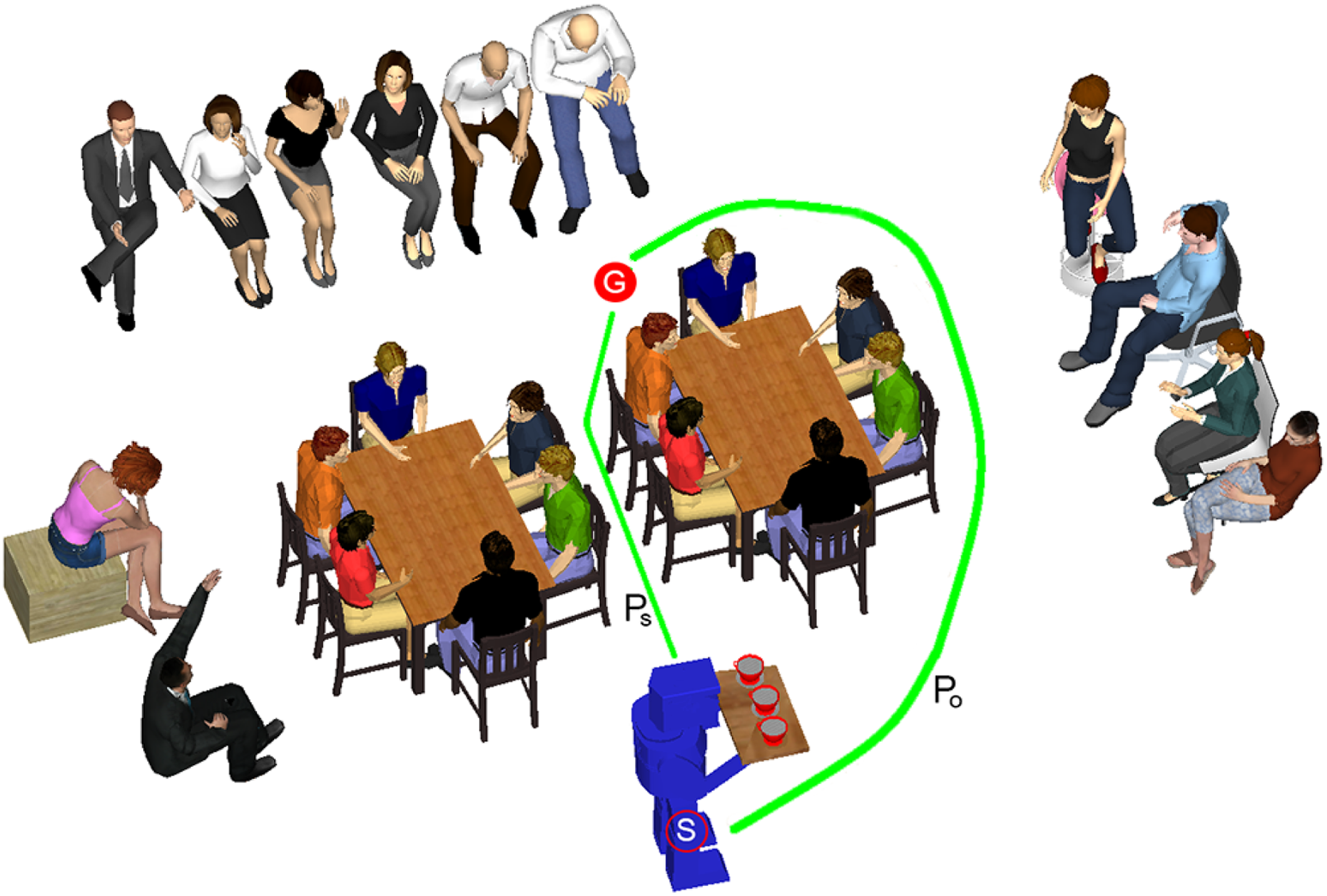
Illustration of human experience–inspired path planning. In this scene, a service robot carrying several cups of coffee on a plate is serving at a party and is required to traverse from the current position S to the target position G. The shortest path Ps is selected by the traditional algorithms, and the path Po is selected by the human experience–inspired algorithm.
In fact, a large number of robots has been built that explicitly mimic biological navigation behaviors for obstacle avoidance, such as the ones emulating an annual migration of seabirds 19,20 and ant-like behavior navigation model. 21 Inspired by the social interactions in human crowds or animal swarms, Savkin and Wang 22 proposed an efficient obstacle avoidance algorithm in dynamic environments by integrating representation of the information about the environment. Typically, the development of robotics has been directly or indirectly affected by human’s experiences and behaviors. 23 –25 However, these methods 24 –27 mainly focus on the motion modeling of robot’s body parts (e.g. arms) and the interactive applications between robots and humans. In this article, we emphasize and learn from human driving experiences. Let’s take some discussion on the human’s driving experiences. Generally, a person prefers reducing the driving speed when passing neighboring areas of obstacles, while speeding up in wide areas with safe enough distance to obstacles. Furthermore, in front of a very narrow aisle, a person like to select another wide path even with a little longer distance. Yet, she/he may determine to continue the narrow path if the wide one is too much long compare with the narrow one. Passive human walking has been studied by many researchers, 28 and it simulates human’s behavior by considering the potential energy consuming when human walking. In a word, path planning by humans is not only related to the time cost, path distance, and ease steering but also relevant to the safety.
Inspired by human’s experiences, we develop a safety-related path planning method. We construct a speed field that can efficiently simulate slowing down and detouring behaviors of humans around obstacles and then integrate the distance and smoothness factors with the speed field to form a human experience–inspired energy function model. Based on this model, the optimal path can be efficiently achieved by the well-known A* algorithm. Specially, the lower bound of the energy function, namely the admissible function in A* algorithm, can be easily estimated. We also propose a fast yet effective post-processing to smooth paths generated by the A* method. In summary, the main contributions of this article include: A human experience–inspired path planning algorithm that considers the safety factor is presented. A dynamic speed field is constructed to control robot’s speed, which can also adapt to dynamic scenes. An effective post-processing approach is utilized to smooth paths for ease steering of robots.
The rest of this article is organized as follows. In “Related work” section introduces some related works. In “The proposed model” section, an energy functional model of path planning is presented to simulate human’s experience, and speed field computation and a practical feasible curvature computation scheme are also detailed. In “Path planning scheme” section, A* algorithm is applied to the energy function to search an optimal path, and a path smoothing method is also presented. Several path evaluation criteria are introduced in “Path evaluation” section. Experimental results are shown in “Implementation and results” section. Finally, conclusions are made in “Conclusions and future works” section.
Related work
Path planning has been widely studied by robot communities and other researchers, and plenty of methods have been proposed to deal with practical problems. In this section, we mainly focus on representative path planning algorithms in two dimensional scenarios, and more references can be found in the study by LaValle. 1
Visibility graph 29,30 views obstacles in configuration spaces as polygons and then constructs a graph using the start position, the goal position, and vertices of polygons. Then the path is obtained by graph search methods, for example, Dijkstra’s algorithm.
Artificial potential field (APF) 7,13,31,32 is another important method for path planning in robots. In general, obstacles are modeled as repulsive fields in APF, while the goal position is considered as an attractive field. Thus, the repulsive fields avoid agents approaching to obstacles, and the attractive fields move agents to the goal. Paths generated by APF are generally smooth, but the main drawback of APF is that a local minimizer is trapped possibly.
Probabilistic path planning algorithm is an effective method, and its two representative methods are the PRM 14 and the RRT. 15,16,33 The basic idea of probabilistic path planning is to randomly select non-collision points in free motion space and then connect them to get a path. Probabilistic methods are probabilistically complete, and the path generated by them for the same problem is also not unique.
A* method 5,11 is a widely used path planning method since it has many good properties: (1) given start and goal positions in a scene, the path achieved by A* is unique; (2) in a finite time, A* can always return a result even there is no solution; and (3) a good admissible function can lead to an acceptable time-consuming even for a large map. Now many researchers have developed various variants of A* to deal with different situations and tasks, such as D* Lite, 34 any-angle A*, 3 and Field D*. 12
Gradient-based methods 35,36 are a two-step algorithm of designing an optimal path. It first uses a straight line to connect the start and target points (even pass through obstacle regions) and then takes points out of obstacles in the gradient directions. Generally, the raw paths generated by the process are not smooth, thus a post smoothing operation is desired.
When an agent faces a completely unknown environment and equips with some sensors, it requires to deal with all kinds of situations according to the sensed information. In the case, machine learning-based methods 17,18 are a good technology to deal with path planning tasks.
Comparing with other path planning algorithms, A* algorithm is a deterministic and flexible approach, and it is very convenient to search an optimal solution for a concrete path planning problem. In this article, we propose using the A* algorithm to optimize the proposed path planning model.
Our method is partially similar to Dolgov et al.’s method, 10 and both methods consider the practical safe requirement, but their method does not consider the distance factor and causes the generated paths often along with central lines of roads. As compared, our method can flexibly adjust the path by controlling parameters of the speed field.
The proposed model
In this section, we introduce the energy function of our path planning method according to human experiences.
Energy function
The driving path of a person is related to both the smoothness and the psychological speed of the path. Generally, people prefer driving on a wide road with high speed, which motivates us to design the energy function E inversely proportional to the speed v. However, when v is too small,

where M > 0 is a large enough constant.
On the other hand, humans are prevailing to smooth paths with little turnings. An ideal case is that the driving road is almost straight. In fact, the steering experience implies two factors: the driving time is as short as possible, and the driving road is as straight and smooth as possible. Let s be the driving distance, and κ is the path smoothness parameter. We also consider that the energy function E is proportional to the distance s and the parameter κ.
According to the above analysis, the energy cost along a path C is defined as follows
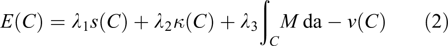
where da represents the line element; λ1 > 0, λ2 > 0, and λ3 > 0 are three trade-off parameters. The energy function relates to two initial conditions, the start position ps and the target position pg. The inequality v ≤ Vmax is also required, where v and Vmax are the scalar values of velocity v(p) and maximal velocity, respectively. We then denote them as the speed and the maximal speed, respectively. κ(C) represents the sum of curvatures along a path C, and v(C) represents the speed sum along a path C.
The objective of this article is to seek an optimal path C* which minimizes the energy cost function defined in equation (2). We also denote the minimal energy as E(C*). Supposing a path

where κ(p) and v(p) are the curvature and speed at point p, respectively.
So far, we have three unknowns s(C), κ(p), and v(p). In the following sections, we give methods to determine the last two quantities. The distance s(C) can be determined by the algorithm automatically.
In the following two subsections, we mainly give details how to compute the speed field v(p) and the computation of curvatures κ(p) at every point p. Here, we just concern the scalar values of v(p) and κ(p).
Dynamic speed field
We assume the map for a robot traversing is a white and black image. The black patches represent obstacles that robots cannot reach, and white parts are available areas that robots can reach.
As we have pointed out, the driving speed of humans is related to driver’s psychology. The speed is high if there are no obstacles around, otherwise it is slow. Thus, the speed is related to the distance between vehicles and obstacles. Therefore, we use the Laplacian equation defined in equation (4) to estimate an impact coefficient map u for an input map. Then u can be viewed as a smooth control function which can simulate the speed field with the maximal speed Vmax

where u(x, y) has the following approximation scheme

where k is the iterative step. The initial conditions are boundaries of obstacles with value 0. The coefficient map is calculated by equation (5) using iterative optimization. In our experiments, the number of iterations is set to 40.
Assuming the maximal speed of a robot as Vmax, the speed field of an input map for a robot is defined as follows

where 0 < ω ≤ 1 is a trade-off coefficient which can control the speed of a robot further.
In practical situations, it is required that the speed of robots is not too slow even it is turning. Thus, the speed field is finally defined by

where 0 < ε < 1 is a constant that control the minimal speed of robots. Essentially, the truncated definition ensures the speed of a robot not too small. Due to the smoothness of Laplacian interpolation, there is not enough discrimination for neighbors of a point in speed map v′. Therefore, a logarithm transformation is performed, and the final speed map is
Dynamic updating
We have presented a static speed field in scenes as earlier, but in practice, dynamic scenes are ubiquitous (e.g. diverse activities of humans) and thus a dynamic updating scheme is required for modern robots with sensors.
For a given map with obstacles O, we first compute the Voronoi diagram Vd of O. If robots detect a new obstacle Os, we then update Vd for Os locally. Denote Cs the Voronoi cell of Os, then the speed field v(x, y) is also updated locally in Cs by the Laplacian equation (5) with zero boundaries of Os.
Curvature computation
As shown in Figure 3, p and q are two points on a curve (blue solid curve), and q is also a neighbor point of p. l′1 and l2 (two green vectors in Figure 2) are two unit tangent lines at p and q, respectively. Translating l′1 to q gets another vector l1, and

where ∥ p − q ∥ is the Euclidean distance of p and q. In this article, we use tangents to approximate curvatures.
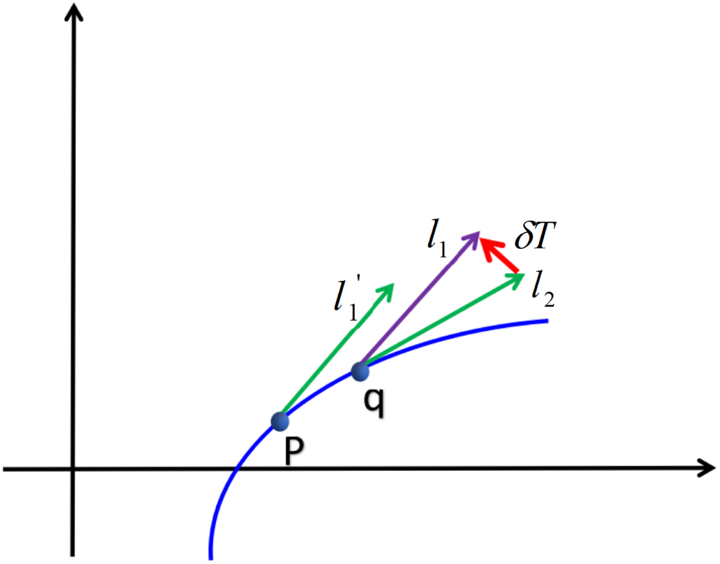
Curvature definition by tangent. l′1 and l2 are the unit tangents of p and q, and translating l′1 to q generates the purple vector l1. δ T is the difference between l1 and l2.
Supposing a robot has been moved i steps which generates i points in the motion space, which are denoted by

where

A benefit of the definition of
Path planning scheme
Based on the proposed model, we search a path by using the A* method that can navigate a robot from any initial position to the target position avoiding collisions.
Formulation in motion space
In this article, robots are assumed to be disk-shaped objects, and obstacles are convex or concave polygons. Assuming a robot centered at x ∈ R2 with radius R > 0 operates in a closed compact space S ⊂ R2, and M polygonal obstacles
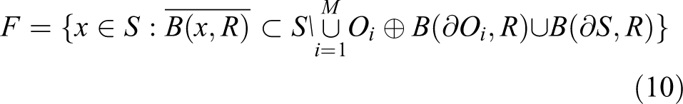
where B(x, r) is an open ball

where
Overall, a robot in theory can walk freely in its free motion space, however, in practice, a more wider space is needed for robots especially when they traverse some obstacles. For example, in Figure 2, rail-mounted robots in an unmanned dinning room generally preserve a certain distance from tables and chairs for safety considerations.
A*-based path planning
Given a target location pg ∈ F and a robot locates at ps ∈ F, we need to find a path that can navigate a robot from ps to pg without collisions. The task can be accomplished by getting a position vector
The A* method selects a path that minimizes

where ∥ ⋅ ∥ is the 2-norm. The heuristic function h(p) designed here is admissible obviously.
On the other hand, if let pk = p, then the function g(p) is defined as

where ss(p) is the length of a polyline
Based on aforementioned formulations, the optimal path can be produced using the standard A* algorithm.
Path smoothing
In most cases, the raw paths generated by A* algorithm are possibly not smooth enough, even the smoothness has been considered. Therefore, a post smooth process is performed to ease driving for robots. Specifically, the path is smoothed by minimizing an energy function under following constraints: (1) paths are smooth enough, (2) point positions in the smoothed path after smoothing are not too far away from original corresponding ones, and (3) smoothed path should also have a strong safe distance to the obstacles.
Assuming the path

where β1, β2 > 0 both are real numbers,
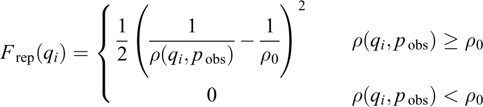
where ρ(·, ·) is the distance function, pobs represents obstacles, and ρ0 > 0 is a constant given by users. The second term of equation (14) guarantees that smoothed paths cannot deviate from original ones too far. The third term guarantees the strong safe distance. The first term attracts the point qi to a Bezier point Bi, which can control the smoothness of the path. Specially, Bi is a Bezier point interpolated by four neighbor points
This formula indicates that Bi is from a cubic Bezier curve. Since Bezier curves are generally smooth, we can desire paths processed by this method are also smooth. In fact, Bezier-based smoothing path generation methods are extensively used in path planning. 37,38
Using the gradient descent algorithm, the energy functional shown in equation (14) can be optimized by the following iterative scheme

where
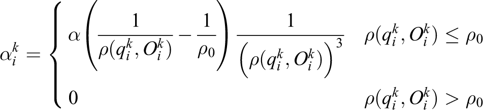
where
Path evaluation
Path Evaluation is very important in path planning study. In the previous work, researchers usually used the following three criteria to measure a path’s quality: the running time T of algorithm, the number of turning points TPN, and the length of a path PL. However, all three aspects do not related to safety. Thus we design following two criteria to measure safety: the minimal distance between a path P and obstacles O: the safety coefficient of a path P and obstacles O:
MD reflects the worst case of a path passing through obstacle regions. SC is used to measure the safety performance which is not considered by previous works to the best of our knowledge. In practice, humans generally desire the path length PL as short as possible and distances to obstacles as long as possible. Therefore, a bigger SC reports a better safety performance.
Implementations and results
In this section, we give implementation details of our algorithm and show the results from our approach. All examples shown in this article are performed on a laptop running on a 3.40 GHz laptop computer with 4 GB of memory. Generally, the path planning algorithm, including A* search and path smoothing, can be accomplished in 0.3 s for an indoor layout map (1026 × 800) and the Paris rendering map (907 × 728) shown in Figures 5 and 6, respectively.
In our implementation, the A* method searches eight directions (8-neighbors) of current position each time, and therefore the step length of every action is 1 or
The proposed optimal path planning algorithm is built on the platform of Visual C++ with Qt 5.3.2 GUI. In the system as shown in Figure 4, we implement the shortest path method and our method, respectively, which are both optimized by the A* search algorithm. On the left working area of the system interface, maps and paths are shown, and the start and target positions S and G can be chosen interactively. On the right panel of the system interface, several widgets are designed to adjust parameters. Once a start position and a target position are chosen, we can choose an algorithm in the process menu to generate a path. For example, in Figure 4, we use our method to generate a path (green curve) that connects S and G.

The interface of our optimal path planning system. The green and blue curves represent our optimal path and the shortest path, respectively.
Experimental results
For given start and target nodes ps = 248, 110 and pg = 669, 653, the example for an indoor scene is shown in Figure 5. The result indicates that our path planning method is feasible for indoor environments. The path (green curve in Figure 5) generated by our method is smooth and extends along boundaries of obstacles, which is very similar to human’s walking habit. Furthermore, the path indeed has a certain distance with boundaries of obstacles, which guarantees strong safety for robot steering. Therefore, it is suitable for robot steering along the path.

Illustration of path planning by our method at an indoor layout scene.
We have also tested the path planning on large-scale scenes. We download a three-dimensional (3-D) Paris model from Internet, and then the model is projected onto the x − z plane orthogonally. The projection is shown in the left of Figure 6. Then the projection is binarized with color clustering operations and manual refinement to extract the transportation road networks of Paris. As shown in Figure 6, red dots indicate the start position (ps = 154, 579) and the target position (pg = 853, 159), and the green and blue curves represent our optimal path and the shortest path, respectively. Note that in this example, the path smoothing is not performed since the width of the road networks is very thin. Note that our path (green curve in Figure 6) contains a long and straight segment comparing with the shortest path (red curve in Figure 6).

Path planning on a large-scale scene. The left is the render map of Paris 3-D model with several path planning results, where the green and blue curves represent our optimal path planning result and the shortest path planning result, respectively. The right-top and the right-bottom are two local zoom-in images.
Path evaluation
We evaluate different paths generated by different path planning algorithms, including RRT method, 16 practical method, 10 fuzzy logic (FL) method, 39 and our method. RRT 16 and the practical search (PS) method 10 are implemented using Matlab [version 2010], and the FL method 39 is implemented by C++. Note that in Figure 7, we set λ3 = 2.0. Paths generated by other methods are smoothed except for RRT, thus a simple mean value filter is used for RRT. Path planning results of these algorithms in maps with size 500 × 500 are shown in Figure 7.

To evaluate path’s quality, five different criteria (see “Path evaluation” section) are computed for paths generated by different algorithms, and the statistical results are reported in Tables 1 and 2. Since RRT is a random algorithm, it is tested ten times in the two static maps, and only one of the results are shown in Figure 7. As shown, RRT method 16 has less turning points comparing to other three algorithms but performs worse with respect to other criteria, especially getting lower safe coefficient. FL method 39 shows a mediocre performance for these criteria. The practical method 10 and our method have a similar safe performance, but our method always have a shorter path length than the practical method. In summary, the method proposed in this article can balance different requirements.
Statistical results of paths are shown in Figure 7(a) to (c), where — means the algorithm fails for the map with given start and target nodes.

RRT: rapidly exploring random tree; FL: fuzzy logic; PS: practical search; TPN: number of turning points; PL: length of a path; MD: minimal distance; SC: safety coefficient.
Statistical results of paths are shown in Figure 7(d) to (g).

RRT: rapidly exploring random tree; FL: fuzzy logic; PS: practical search; TPN: number of turning points; PL: length of a path; MD: minimal distance; SC: safety coefficient.
We have also analyzed influence of different parameters λ1, λ2, and λ3 for optimal path planning, as shown in Figure 8. In this example, we generally set λ1 = 0.01, λ2 = 0.01, and λ3 = 0.01 if without special explanation. The paths shown in Figure 8(a) to (d) tend to be a shorter one with increasing λ1, which agrees with our model designing. With the increasing of λ2, paths shown in Figure 8 (e) to (h) have obvious variations. In fact, since curvature characterizes local shapes of geometry, and it is also very sensitive, thus different λ2 lead diverse results. There is a little special for λ3. When it is bigger than λ1 and λ2, paths shown in Figure 8 (j) to (l) do not show obvious variations. Therefore λ3 is not sensitive if it has a bigger value. Hence choices of λ1, λ2, and λ3 are pivotal for concrete applications. We could set a larger λ1 for a shorter distance requirement. Note that λ2 controls the weight of curvatures of paths which are a local geometrical features. Therefore, we advise a large λ2 if a local smoothness is desired. However, a very large λ2 is not a good choice for smoothness (e.g. Figure 8(g) and (h)). Generally, we suggest a large value of λ3 and a similar value of λ1 and λ2 for a safe path application.
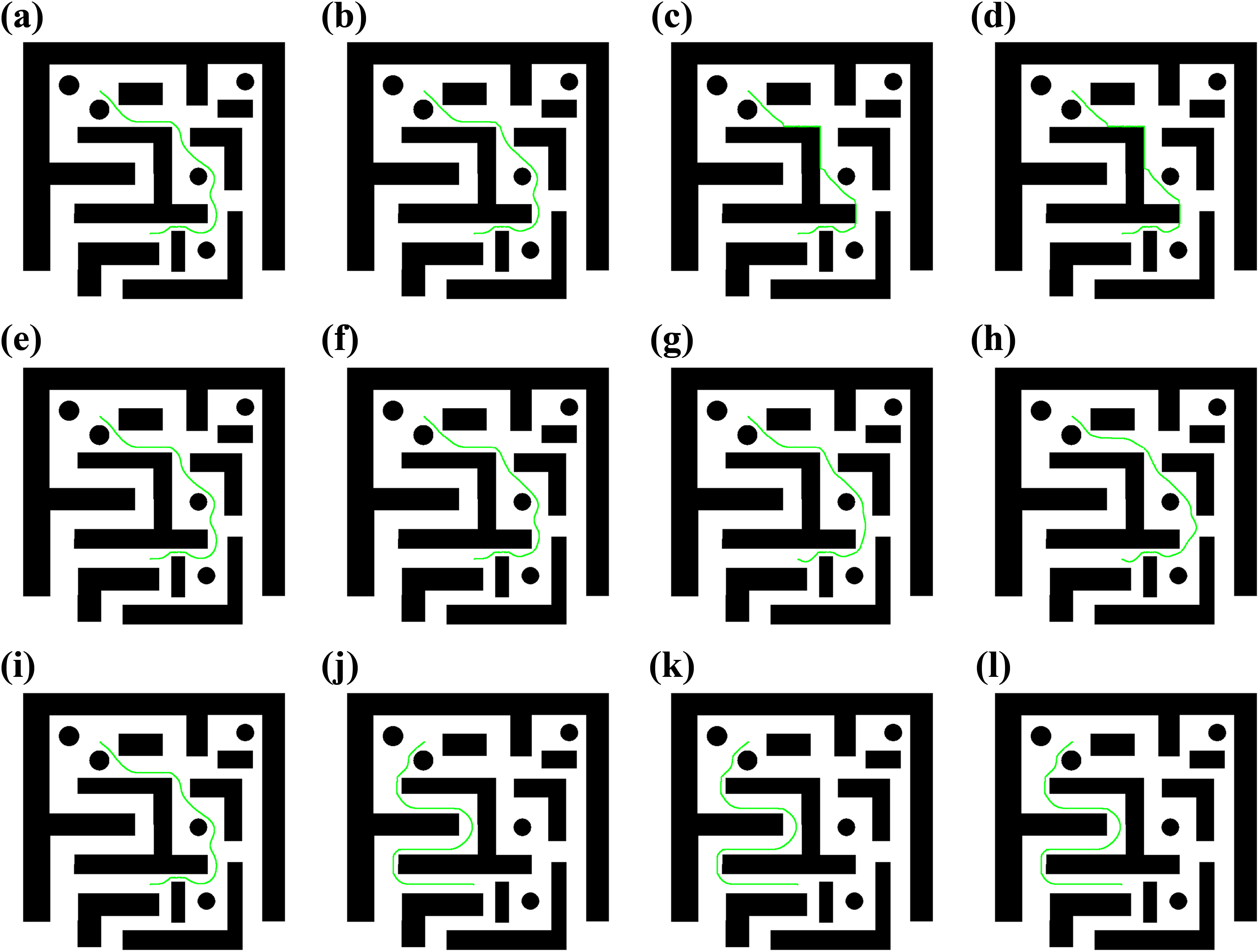
The path planning results by our method with different parameters. (a) λ 1 = 0.01; (b) λ 1 = 0.05; (c) λ 1 = 0.5; (d) λ 1 = 3; (e) λ 2 = 0.01; (f) λ 2 = 0.05; (g) λ 2 = 0.5; (h) λ 2 = 3; (i) λ 3 = 0.01; (j) λ 3 = 0.05; (k) λ 3 = 0.5; and (l) λ 3 = 3.
Dynamic scenes
A dynamic path planning example is tested, and the result is shown in Figure 9. A path is generated and connects S and G in a static scene shown in Figure 9(a). But in Figure 9(b), when robots move to the node M, a new obstacle H is detected, and then the speed field is updated, and the path is also re-computed. The final path is shown in Figure 9(b). The example illustrates that the dynamic updating scheme is useful for dynamic scenes.

Illumination of path planned in dynamic scene by our method. Compared with (a), a new obstacle H appears in (b).
Examples shown in this section demonstrate that our optimal path planning algorithm for robots is practically feasible. Specially, these results also validate that our model can simulate human’s experiences.
Conclusions and future works
In this article, we propose a model to simulate human’s path planning. Specially, the safety of robot navigation is considered. The major technical contributions of the article include the following aspects: A dynamic speed field is proposed, which is incorporated with multiple factors, such as safety, path curvatures and path distance, to model human driving experiences. By adapting parameters (λ1, λ2, λ3), the model can generate diverse paths according to specific requirements. An efficient but easy-to-implement path smoothing algorithm is presented. The smoothed path is more suitable for steering of robots. Experiments on indoor scene and large-scale outdoor scene have demonstrated the effectiveness of our path planning method.
In the future, we would like to develop our method in several aspects, such as smartly selecting parameters λ1, λ2, and λ3, and adapting to usual maps (e.g. maps with non-smoothed obstacles). We also would like to develop our method assisted by scene sematic analysis especially identifying the static objects and persons.
Footnotes
Acknowledgements
We would like to give our thanks to the artist Johnny who shares the 2-D indoor layout map (Figure 5), and Konstantin who shares the 3-D Paris model (![]() ).
).
Declaration of conflicting interests
The author(s) declared no potential conflicts of interest with respect to the research, authorship, and/or publication of this article.
Funding
The author(s) disclosed receipt of the following financial support for the research, authorship, and/or publication of this article: This project was partially supported by the Natural Science Foundation of China (no. 61672544, 61725204, 61661130156), Guangdong Natural Science Foundation (no. 2015A030311047), Tip-top Scientific and Technical Innovative Youth Talents of Guangdong special support program (no. 2016TQ03X263), the Fundamental Research Funds for the Central Universities (no. 11617348), Beijing Higher Institution Research Center of Visual Media Intelligent Processing and Security, and Foundation of Key Laboratory of Machine Intelligence and Advanced Computing of the Ministry of Education (no. MSC-201701A), and Shenzhen Innovation Program (no. JCJY2015040114529008).