Sage Journals: Discover world-class research

Abstract

It is impossible to achieve vertex movement and rapid velocity control in aerial robots and aerial vehicles because of momentum from the air. A continuous-curvature path ensures such robots and vehicles can fly with stable and continuous movements. General continuous path-planning methods use spline interpolation, for example B-spline and Bézier curves. However, these methods cannot be directly applied to continuous path planning in a 3D space. These methods use a subset of the waypoints to decide curvature and some waypoints are not included in the planned path. This paper proposes a method for constructing a curvature-continuous path in 3D space that includes every waypoint. The movements in each axis, x, y and z, are separated by the parameter u. Waypoint groups are formed, each with its own continuous path derived using quadratic polynomial interpolation. The membership function then combines each continuous path into one continuous path. The continuity of the path is verified and the curvature-continuous path is produced using the proposed method.

Keywords

Aircraft navigation Continuous path Interpolation Mobile robot Path planning Robot motion Path-smoothing algorithm Unmanned aerial vehicles

1. Introduction

Path searching is one of the main topics in path-planning research. The primary purpose of path planning is to construct a collision-free path. Commonly used algorithms for path planning include the D^* algorithm [1], potential field algorithm [2], Probabilistic Roadmap Methods (PRM) algorithm [3], and Rapidly exploring Random Trees (RRT) [4]. These algorithms focus on path planning on a 2D plane. For path planning in a 3D space, researchers have proposed algorithms to create various optimal or sub-optimal paths [5] [6]. These algorithms provide a method of creating paths using waypoints for the 3D movement of aerial vehicles and aerial robots [7].

Many forces, such as gravitational, centrifugal, centripetal, and inertia, may obstruct stable movement in a real physical environment. These forces have a greater effect on movements in a 3D space compared to movements on a 2D plane. On a 2D plane, the movements obtain momentum from the ground. Therefore, as long as slippage does not occur or the path is continuous, the effects of these forces can be neglected. On the other hand, in a 3D space the movement of aerial robots or aerial vehicles is unable to obtain momentum from the ground. Instead, momentum is gained from the air; for this, a fixed-wing aircraft must have a larger velocity than stalling velocity [8]. If the velocity drops below the stalling velocity, the fixed-wing aircraft cannot obtain the lift force and will stall. Therefore, the fixed-wing aircraft must fly above the stalling velocity and cannot have any sharp angular movements or stop in the 3D space. A rotary-wing aircraft can hover in 3D space but cannot have any sharp angular movement or rapidly stop. These conditions imply that the movements of aircraft in 3D space should not have vertexes and that the velocity and acceleration should be continuous and maintained above the stalling velocity.

Paths with continuous velocity and acceleration, also referred to as smooth paths or continuous paths, are classified in terms of continuity, G⁰, G¹, G², -, Gⁿ [9]. A G⁰ continuous path is constructed by forming a straight line between the waypoints. PRM [3] produces the G 0 continuous path. A G¹ continuous path matches the first-order differential values at each of the waypoints. This path provides a continuous velocity and a common tangential direction at the waypoint. A G² continuous path has the same second-order differential values and also shares a common centre of curvature. This path has a continuous acceleration, and it is called a curvature-continuous path. A Gⁿ continuous path is defined as a continuity of the n ^th-order differential values. The path must have G² continuity to guarantee smooth movements.

Many studies focus on movements in 2D space and utilize spline-based methods to construct the continuous path. Magid et al. proposed a robot navigation algorithm based on spline [10]. Komoriya et al. proposed trajectory design and control of a wheel-type mobile robot using B-spline [11]. Piazzi et al. demonstrated the use of $η^{3}$ splines in smooth-path generation for wheeled mobile robots [12]. Berglund et al. explored an obstacle-avoiding minimum variation b-spline problem [13]. Anderson et al. studied real-time trajectory smoothing for unmanned air vehicles in a 2D plane [14]. Jung and Tsiotras applied b-spline to generate a path for small unmanned vehicles in a 2D plane [15].

Various algorithms have also been applied for constructing continuous paths in 3D space. Hasircioglu et al. showed 3D path planning for the navigation of UAV by applying evolutionary algorithms using B-spline [5]. Yang et al. demonstrated a 3D path-smoothing algorithm using cubic Bézier spiral curves [16]. Further, Babaei and Mortazavi described 3D curvature-constrained trajectory planning based on in-flight waypoints [6].

Most 2D and 3D continuous path-planning methods use spline interpolation, for example B-spline and Bézier spiral curves. However, such methods are not applicable in path-smoothing methods because some waypoints are not part of the smoothed path. Instead, control points should be used to decide curvature in the path.

This paper expands the quadratic polynomial interpolation (QPMI) path-smoothing method [17] [18], used for path smoothing in a 2D plane, to connect waypoints and form continuous curves in a 3D space.

The rest of the paper is organized as follows: section 2 explains the path-smoothing method using polynomial interpolation. In section 3, the QPMI path-smoothing method is expanded to apply to the 3D space. Section 4 proposes the membership function for the QPMI path-smoothing method in a 3D space. Section 5 discusses continuity and curvature in the proposed method. Section 6 describes a series of 3D path-smoothing simulations using the proposed method. Section 7 provides conclusions.

2. Path-smoothing method using polynomial interpolation

In the case of aerial robots or aerial vehicles polynomial interpolation cannot be applied directly, because in a 3D space the path involves a complex non-linear trajectory where each waypoint has a visit sequence. The planned path must visit every waypoint in sequential order. These conditions make it difficult to apply polynomial interpolation directly to 3D paths. Other spline-interpolation-based methods produce paths that do not visit all waypoints. Instead, control points are either used based on a subset of waypoints or determined using another method. In this case, the planned smooth path may be a shorter path, but it is not a unique path through the waypoints. Essentially, the path should depend on the waypoints only, and visit all waypoints.

General polynomial interpolation involves constructing a polynomial curve that includes every waypoint. Runge's phenomenon [9] occurs when using high-order polynomials. QPMI [17] avoids Runge's phenomenon by using the quadratic polynomial, which is the lowest-order polynomial connecting three waypoints with G² continuity. In addition, it has a unique solution, a shortest path, and can obtain variations in curvature. These features provide high reliability and require only low-performance hardware. However, in order to create a shortest path, the quadratic polynomial should have a rotated form. QPMI [17] can express a 3D path in the 3D space by improving the parameter u, which denotes the distance of the linear path between the neighbour waypoints. This parameter separates the x, y, and z values from the 3D axes. The values and the differential values of each axis can then be obtained. These values provide the variation of curvature and the continuity.

This paper expands the QPMI path-smoothing method [17] and demonstrates how the proposed method can create a smooth path by combining quadratic polynomials sequentially in the 3D space.

3. Continuous path creation using quadratic polynomials

3.1 Smooth path connecting three waypoints using quadratic polynomial

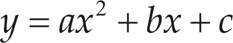
In QPMI [17] the path connecting three waypoints can be expressed using a quadratic polynomial. Equation (1) is the quadratic polynomial for presenting a path on the 2D plane.

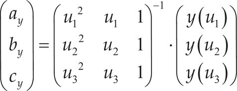
\begin{matrix} P : (x, y) ∊ R^{2} \\ y = a x^{2} + b x + c \end{matrix}

(1)

The quadratic polynomial connecting the three waypoints (P₁:(x₁, y₁), P₂:(x₂, y₂), and P₃:(x ₃, y₃)) can be obtained using the following method:

\begin{array}{l} (\begin{matrix} y_{1} \\ y_{2} \\ y_{3} \end{matrix}) = (\begin{matrix} x_{1}^{2} & x_{1} & 1 \\ x_{2}^{2} & x_{2} & 1 \\ x_{3}^{2} & x_{3} & 1 \end{matrix}) \cdot (\begin{matrix} a \\ b \\ c \end{matrix}) \\ (\begin{matrix} a \\ b \\ c \end{matrix}) = {(\begin{matrix} x_{1}^{2} & x_{1} & 1 \\ x_{2}^{2} & x_{2} & 1 \\ x_{3}^{2} & x_{3} & 1 \end{matrix})}^{- 1} \cdot (\begin{matrix} y_{1} \\ y_{2} \\ y_{3} \end{matrix}) \end{array}

(2)

Equation (2) is an inverse matrix for obtaining the quadratic polynomial. This is the general quadratic polynomial interpolation for connecting three waypoints, which constructs the shortest G² continuous path.

Figure 1.

(a) Quadratic polynomial graph on the 2D plane. (b) Quadratic polynomial connecting three waypoints in the 3D space.

Figure 1 illustrates the quadratic polynomial graph on the 2D plane (a), and, similarly, in the 3D space (b). The waypoints in the 3D space are expressed by equation (3).

P_{n} : (x_{n}, y_{n}, z_{n}) ∊ R^{3}, n = 1, 2, \dots, m

(3)

The aim of this paper is to construct and express smooth paths using quadratic polynomials in the 3D space. To apply this concept to the 3D space, a parametric method is used to express the 3D path.

3.2 Parametric method for 3D path

The parametric method provides a convenient description of the path. The parametric path in the 3D space can be expressed as

P (u) : (x (u), y (u), z (u))

(4)

The parameter u is the linear distance and can be calculated from the linear piecewise path. In the 3D space, there are three waypoints: P₁:(x a t y₁, z ₁), P₂:(x₂, y₂, z₂), and P₃: (x_3, y_3, z₃). The parameter u can then be obtained as:

\begin{matrix} u_{1} = 0 \\ u_{2} = u_{1} + \sqrt{{(x_{2} - x_{1})}^{2} + {(y_{2} - y_{1})}^{2} + {(z_{2} - z_{1})}^{2}} \\ u_{3} = u_{2} + \sqrt{{(x_{3} - x_{2})}^{2} + {(y_{3} - y_{2})}^{2} + {(z_{3} - z_{2})}^{2}} \end{matrix}

(5)

x (u) = a_{x} u^{2} + b_{x} u + c_{x}

(6)

y (u) = a_{y} u^{2} + b_{y} u + c_{y}

(7)

z (u) = a_{z} u^{2} + b_{z} u + c_{z}

(8)

From equations (6), (7), and (8), we obtain the following inverse matrix calculations:

(\begin{matrix} a_{x} \\ b_{x} \\ c_{x} \end{matrix}) = {(\begin{matrix} u_{1}^{2} & u_{1} & 1 \\ u_{2}^{2} & u_{2} & 1 \\ u_{3}^{2} & u_{3} & 1 \end{matrix})}^{- 1} \cdot (\begin{matrix} x (u_{1}) \\ x (u_{2}) \\ x (u_{3}) \end{matrix})

(9)

(\begin{matrix} a_{y} \\ b_{y} \\ c_{y} \end{matrix}) = {(\begin{matrix} u_{1}^{2} & u_{1} & 1 \\ u_{2}^{2} & u_{2} & 1 \\ u_{3}^{2} & u_{3} & 1 \end{matrix})}^{- 1} \cdot (\begin{matrix} y (u_{1}) \\ y (u_{2}) \\ y (u_{3}) \end{matrix})

(10)

(\begin{matrix} a_{z} \\ b_{z} \\ c_{z} \end{matrix}) = {(\begin{matrix} u_{1}^{2} & u_{1} & 1 \\ u_{2}^{2} & u_{2} & 1 \\ u_{3}^{2} & u_{3} & 1 \end{matrix})}^{- 1} \cdot (\begin{matrix} z (u_{1}) \\ z (u_{2}) \\ z (u_{3}) \end{matrix})

(11)

These equations express the G² continuous path in the 3D space using the parametric method. The path has a parabolic curve and the plane of this curve is defined as a triangle made by three waypoints in the 3D space. If variations of each axis are G² continuous, the combined path has G² continuity.

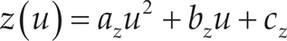
Equation (5) can be generalized as:

\begin{matrix} u_{1} = 0 \\ u_{n} = \sum_{n = 2}^{m} \sqrt{{(x_{n} - x_{n - 1})}^{2} + {(y_{n} - y_{n - 1})}^{2} + {(z_{n} - z_{n - 1})}^{2}} \end{matrix}

(12)

In addition, equations (9), (10), and (11) can be described as follows:

(\begin{matrix} a_{x_{n - 1}} \\ b_{x_{n}} \\ c_{x_{n + 1}} \end{matrix}) = {(\begin{matrix} u_{n - 1}^{2} & u_{n - 1} & 1 \\ u_{n}^{2} & u_{n} & 1 \\ u_{n + 1}^{2} & u_{n + 1} & 1 \end{matrix})}^{- 1} \cdot (\begin{matrix} x_{n} (u_{n - 1}) \\ x_{n} (u_{n}) \\ x_{n} (u_{n + 1}) \end{matrix})

(13)

(\begin{matrix} a_{y_{n - 1}} \\ b_{y_{n}} \\ c_{y_{n + 1}} \end{matrix}) = {(\begin{matrix} u_{n - 1}^{2} & u_{n - 1} & 1 \\ u_{n}^{2} & u_{n} & 1 \\ u_{n + 1}^{2} & u_{n + 1} & 1 \end{matrix})}^{- 1} \cdot (\begin{matrix} y_{n} (u_{n - 1}) \\ y_{n} (u_{n}) \\ y_{n} (u_{n + 1}) \end{matrix})

(14)

(\begin{matrix} a_{z_{n - 1}} \\ b_{z_{n}} \\ c_{z_{n + 1}} \end{matrix}) = {(\begin{matrix} u_{n - 1}^{2} & u_{n - 1} & 1 \\ u_{n}^{2} & u_{n} & 1 \\ u_{n + 1}^{2} & u_{n + 1} & 1 \end{matrix})}^{- 1} \cdot (\begin{matrix} z_{n} (u_{n - 1}) \\ z_{n} (u_{n}) \\ z_{n} (u_{n + 1}) \end{matrix})

(15)

(2 \leq n \leq m - 1)

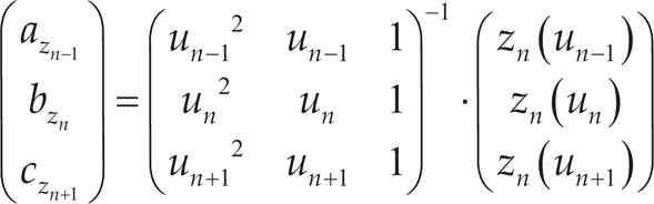
Equations (13), (14), and (15) are the generalized equations of (9), (10), and (11). Path (4) can be changed as follows:

P (u) = {\begin{matrix} q_{2} : (x_{2} (u), y_{2} (u), z_{2} (u)), (u_{1} \leq u_{2} \leq u_{3}) \\ q_{3} : (x_{3} (u), y_{3} (u), z_{3} (u)), (u_{2} \leq u_{3} \leq u_{4}) \\ ⋮ \\ q_{n} : (x_{m - 1} (u), y_{m - 1} (u), z_{m - 1} (u)), (u_{m - 2} \leq u_{m - 1} \leq u_{m}) \end{matrix}

(16)

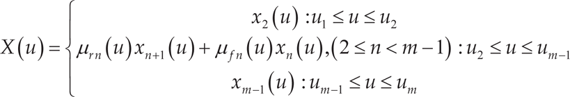
The m^th waypoints require m - 2 polynomials at each axis. In the case of four or more waypoints, the general polynomial interpolation requires an increasing polynomial degree. For four waypoints, two quadratic polynomial paths are available. In this paper, the waypoints are grouped. The first group consists of P₁, P₂, and P₃. The first parametric quadratic polynomials P₂: (x₂(u), y₂(u), z₂(u)) can be obtained by using equations (13), (14), and (15). This path is the G² continuous path connecting P₁, P₂, and P₃. The second group consists of P₂, P₃, and P₄ and the second parametric quadratic polynomials P₃: (x₃(u), y₃(u), z₃(u)) are obtained similarly. These two quadratic polynomial groups overlap between P₂ and P₃. The two paths are then combined using a membership function at the overlapping region.

4. QPMI 3D path-smoothing method

The membership function applied uses a triangular function to distribute the degree of truth in the fuzzy control theory.

Figure 2.

Triangular membership functions. Red dotted line is a variation of P₂(u) degree. Blue dashed line is a variation of P₃(u) degree.

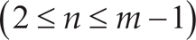
Figure 2 shows variations of the membership functions in the case of four waypoints. The overlapped section P₂ to P₃ is expressed by the parameters u₂ and u₃. The degree of two waypoints varies by parameter u. The red dotted line decreases in the section from u₂ to u₃. In this section, the degree of P₂(u) decreases. The blue dashed line increases in the section from u₂ to u₃. The degree of P3(u) is increasing in this section. The group of paths is defined as

P : (X (u), Y (u), Z (u))

(17)

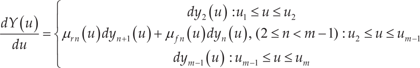
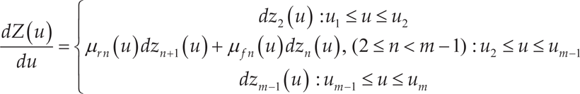
X(u), Y(u) and Z(u) are described as follows:

X (u) = {\begin{matrix} μ_{r}_{1} (u) x_{2} (u) + μ_{f}_{1} (u) x_{1} (u) : u_{1} \leq u \leq u_{2} \\ μ_{r}_{2} (u) x_{3} (u) + μ_{f}_{2} (u) x_{2} (u) : u_{2} \leq u \leq u_{3} \\ μ_{r}_{3} (u) x_{4} (u) + μ_{f}_{3} (u) x_{3} (u) : u_{3} \leq u \leq u_{4} \\ ⋮ \\ μ_{r}_{m - 2} (u) x_{m - 1} (u) + μ_{f}_{m - 2} (u) x_{m - 2} (u) : u_{m - 2} \leq u \leq u_{m - 1} \\ μ_{r}_{m - 1} (u) x_{m} (u) + μ_{f}_{m - 1} (u) x_{m - 1} (u) : u_{m - 1} \leq u \leq u_{m} \end{matrix}

(18)

Y (u) = {\begin{matrix} μ_{r}_{1} (u) y_{2} (u) + μ_{f}_{1} (u) y_{1} (u) : u_{1} \leq u \leq u_{2} \\ μ_{r}_{2} (u) y_{3} (u) + μ_{f}_{2} (u) y_{2} (u) : u_{2} \leq u \leq u_{3} \\ μ_{r}_{3} (u) y_{4} (u) + μ_{f}_{3} (u) y_{3} (u) : u_{3} \leq u \leq u_{4} \\ ⋮ \\ μ_{r}_{m - 2} (u) y_{m - 1} (u) + μ_{f}_{m - 2} (u) y_{m - 2} (u) : u_{m - 2} \leq u \leq u_{m - 1} \\ μ_{r}_{m - 1} (u) y_{m} (u) + μ_{f}_{m - 1} (u) y_{m - 1} (u) : u_{m - 1} \leq u \leq u_{m} \end{matrix}

(19)

Z (u) = {\begin{matrix} μ_{r}_{1} (u) z_{2} (u) + μ_{f}_{1} (u) z_{1} (u) : u_{1} \leq u \leq u_{2} \\ μ_{r}_{2} (u) z_{3} (u) + μ_{f}_{2} (u) z_{2} (u) : u_{2} \leq u \leq u_{3} \\ μ_{r}_{3} (u) z_{4} (u) + μ_{f}_{3} (u) z_{3} (u) : u_{3} \leq u \leq u_{4} \\ ⋮ \\ μ_{r}_{m - 2} (u) z_{m - 1} (u) + μ_{f}_{m - 2} (u) z_{m - 2} (u) : u_{m - 2} \leq u \leq u_{m - 1} \\ μ_{r}_{m - 1} (u) z_{m} (u) + μ_{f}_{m - 1} (u) z_{m - 1} (u) : u_{m - 1} \leq u \leq u_{m} \end{matrix}

(20)

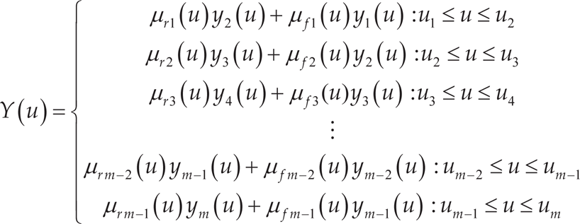
μ_f (u) is a decreasing function and is depicted by the red dotted line in Figure 2. This function starts at one and decreases to zero. On the other hand, μ_r(u) is an increasing function. This function starts at zero and increases to one. The membership functions are as follows.

μ_{r}_{n} (u) = \frac{(u - u_{n})}{(u_{n + 1} - u_{n})}, (1 \leq n \leq m - 1)

(21)

μ_{r}_{n} (u) = \frac{(u_{n + 1} - u)}{(u_{n + 1} - u_{n})}, (1 \leq n \leq m - 1)

(22)

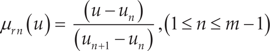
Since there is no overlap in the first and last sections, the polynomials are not affected by other polynomials and the membership function is not required. Therefore, μ_r(u) and μ_fm−1(u). are both one. The general functions 1 can be described as:

X (u) = {\begin{matrix} x_{2} (u) : u_{1} \leq u \leq u_{2} \\ μ_{r}_{n} (u) x_{n + 1} (u) + μ_{f}_{n} (u) x_{n} (u), (2 \leq n < m - 1) : u_{2} \leq u \leq u_{m - 1} \\ x_{m - 1} (u) : u_{m - 1} \leq u \leq u_{m} \end{matrix}

(23)

Y (u) = {\begin{matrix} y_{2} (u) : u_{1} \leq u \leq u_{2} \\ μ_{r}_{n} (u) y_{n + 1} (u) + μ_{f}_{n} (u) y_{n} (u), (2 \leq n < m - 1) : u_{2} \leq u \leq u_{m - 1} \\ y_{m - 1} (u) : u_{m - 1} \leq u \leq u_{m} \end{matrix}

(24)

Z (u) = {\begin{matrix} z_{2} (u) : u_{1} \leq u \leq u_{2} \\ μ_{r}_{n} (u) z_{n + 1} (u) + μ_{f}_{n} (u) z_{n} (u), (2 \leq n < m - 1) : u_{2} \leq u \leq u_{m - 1} \\ z_{m - 1} (u) : u_{m - 1} \leq u \leq u_{m} \end{matrix}

(25)

The polynomial is obtained by finding the quadratic polynomial's solution using the 3×3 inverse matrix, which has a unique and simple solution without high-order polynomials and trigonometric functions. On the other hand, the quadratic polynomials have the cubic polynomial form at the overlapped sections using the membership functions.

5. Continuity and curvature

Path continuity is determined by differential values. If the first-order differential values connect each waypoint, the path is the G¹ continuous path. If the second-order differential values match at each waypoint, the path is the G² continuous path. The first-order differential values of X (u), Y(u), and Z(u) can be obtained as:

\frac{d X (u)}{d u} = {\begin{matrix} d x_{2} (u) : u_{1} \leq u \leq u_{2} \\ μ_{r}_{n} (u) d x_{n + 1} (u) + μ_{f}_{n} (u) d x_{n} (u), (2 \leq n < m - 1) : u_{2} \leq u \leq u_{m - 1} \\ d x_{m - 1} (u) : u_{m - 1} \leq u \leq u_{m} \end{matrix}

(26)

\frac{d Y (u)}{d u} = {\begin{matrix} d y_{2} (u) : u_{1} \leq u \leq u_{2} \\ μ_{r}_{n} (u) d y_{n + 1} (u) + μ_{f}_{n} (u) d y_{n} (u), (2 \leq n < m - 1) : u_{2} \leq u \leq u_{m - 1} \\ d y_{m - 1} (u) : u_{m - 1} \leq u \leq u_{m} \end{matrix}

(27)

\frac{d Z (u)}{d u} = {\begin{matrix} d z_{2} (u) : u_{1} \leq u \leq u_{2} \\ μ_{r}_{n} (u) d z_{n + 1} (u) + μ_{f}_{n} (u) d z_{n} (u), (2 \leq n < m - 1) : u_{2} \leq u \leq u_{m - 1} \\ d z_{m - 1} (u) : u_{m - 1} \leq u \leq u_{m} \end{matrix}

(28)

The second-order differential values are described as:

\frac{d^{2} X (u)}{d u} = {\begin{matrix} d^{2} x_{2} (u) : u_{1} \leq u \leq u_{2} \\ μ_{r}_{n} (u) d^{2} x_{n + 1} (u) + μ_{f}_{n} (u) d^{2} x_{n} (u), (2 \leq n < m - 1) : u_{2} \leq u \leq u_{m - 1} \\ d^{2} x_{m - 1} (u) : u_{m - 1} \leq u \leq u_{m} \end{matrix}

(29)

\frac{d^{2} Y (u)}{d u^{2}} = {\begin{matrix} d^{2} y_{2} (u) : u_{1} \leq u \leq u_{2} \\ μ_{r}_{n} (u) d^{2} y_{n + 1} (u) + μ_{f}_{n} (u) d^{2} y_{n} (u), (2 \leq n < m - 1) : u_{2} \leq u \leq u_{m - 1} \\ d^{2} y_{m - 1} (u) : u_{m - 1} \leq u \leq u_{m} \end{matrix}

(30)

\frac{d^{2} Z (u)}{d u^{2}} = {\begin{matrix} d^{2} z_{2} (u) : u_{1} \leq u \leq u_{2} \\ μ_{r}_{n} (u) d^{2} z_{n + 1} (u) + μ_{f}_{n} (u) d^{2} z_{n} (u), (2 \leq n < m - 1) : u_{2} \leq u \leq u_{m - 1} \\ d^{2} z_{m - 1} (u) : u_{m - 1} \leq u \leq u_{m} \end{matrix}

(31)

On the x axis, the x_n (u) is the quadratic polynomial connecting the (n−1) ^th, n^th, and (n + 1)^th waypoints. This polynomial has maximum degree at the n^th waypoint. At the n^th waypoint, x_n (u) exists and the differential values of x_n (u) are only affected at the n^th waypoint. Therefore, the first-order and second-order differential values at the n^th waypoint are decided by x_n (u). This means the path is the G ² continuous path. The y_n(u) and z_n (u) can be described as the case of x_n (u). These values are as follows:

\frac{d x_{n}}{d u} = 2 a_{x_{n}} u + b_{x_{n}}, \frac{d^{2} x_{n}}{d u^{2}} = 2 a_{x_{n}}

(32)

\frac{d y_{n}}{d u} = 2 a_{y_{n}} u + b_{y_{n}}, \frac{d^{2} y_{n}}{d u^{2}} = 2 a_{y_{n}}

(33)

\frac{d z_{n}}{d u} = 2 a_{z_{n}} u + b_{z_{n}}, \frac{d^{2} z_{n}}{d u^{2}} = 2 a_{z_{n}}

(34)

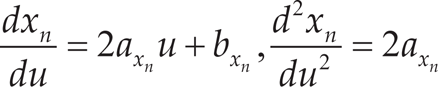
Equations (32), (33), and (34) show the first-order and second-order differential values at the n^th waypoint.

The curvature is related to the differential values. The curvature of the parametric quadratic polynomial can be described by equation (35) using equations (26) to (31).

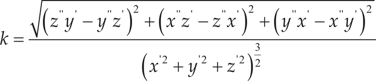
k = \frac{\sqrt{{(z^{″} y^{′} - y^{″} z^{′})}^{2} + {(x^{″} z^{′} - z^{″} x^{′})}^{2} + {(y^{″} x^{′} - x^{″} y^{′})}^{2}}}{{(x^{′ 2} + y^{′ 2} + z^{′ 2})}^{\frac{3}{2}}}

(35)

Equation (35) consists of the differential values and is a function of u. The continuity of curvature is an important part in constructing the smooth path. The G² continuous path is called the curvature continuous path. The continuous curvature is necessary to verify G² continuity. If the curvature graph is continuous, this path is the G² continuous path.

6. Simulation

6.1 Movement of aerial robot in the 3D-space

This simulation assumes that the aerial robot requires a smooth 3D path. Table 1 shows ten waypoints. The proposed method is applied to construct the smooth 3D path from the waypoints and the continuity of the planned 3D path is then verified. In addition, variations of each axis and curvature are obtained.

Table 1.
Waypoints for simulation

	P₂	P₃	P₄	P₅	P₆	P₇	P₈	P₉
x	20	50	80	90	80	50	20	20
y	10	20	20	50	80	80	60	40
z	15	20	15	20	15	20	15	10

This path starts at the origin. The aerial robot flies around an area with variable elevation and returns to the origin. To apply the proposed method, the parameter u was obtained using equation (12).

Table 2.

Parameter u for simulation

u₁	u₂	u₃	u₄	u₅
0	26.93	58.94	89.35	121.37
u₆	u₇	u₈	u₉	u₁₀
153.39	183.80	220.20	240.82	286.64

6.2 3D smooth path planning

The general linear path is shown in Figure 3. In this simulation, we change this linear piecewise path to the G 2 continuous path.

Figure 3.

Linear piecewise path of aerial robot

The first step requires finding variations of x, y, and z using equations (23), (24), and (25). These variations are shown in Figure 4.

Figure 4.

(a) Variation of the x axis. (b) Variation of the y axis. (c) Variation of elevation in the z axis

Figure 5 shows the path on the 2D plane using the variations of x and y. The variation of z is in accordance with the altitude of the aerial robot.

Figure 5.

Aerial robotm's movement on the 2D plane

The 3D path is formed by expressing the path as shown in Figure 5 along with the altitude in the 3D space. Figure 6 displays the 3D path using the proposed method.

Figure 6 has a continuous form, but determining whether it is a G² continuous path requires checking the continuity of the path.

Figure 6.

3D smooth path using the proposed method

6.3 Checking continuity

Continuity can be determined by the first-order and second-order differential values. The graph of the first-order differential values is shown in Figure 7 and the graph of second-order differential values is shown in Figure 8.

Figure 7.

Graphs of the first-order differential values: (a) is the x, (b) is the y and (c) is the z axis

Figures 7 and 8 show continuous graphs in all the axes Since there are no disjointed sections visible in the graphs, the path has G² continuity

These values can create the curvature by using equation (35). The graph of curvature is shown in Figure 9.

The G² continuous path has continuous curvature The planned path in Figure 9 also has continuous curvature The section in which the curvature changes in Figure 9 matches the variation shown in Figure 6 Therefore the planned 3D smooth path is the G² continuous path.

The simulation showed that the proposed method constructs the 3D G² continuous path from the waypoints The continuity is verified by checking the differential values.

Figure 8.

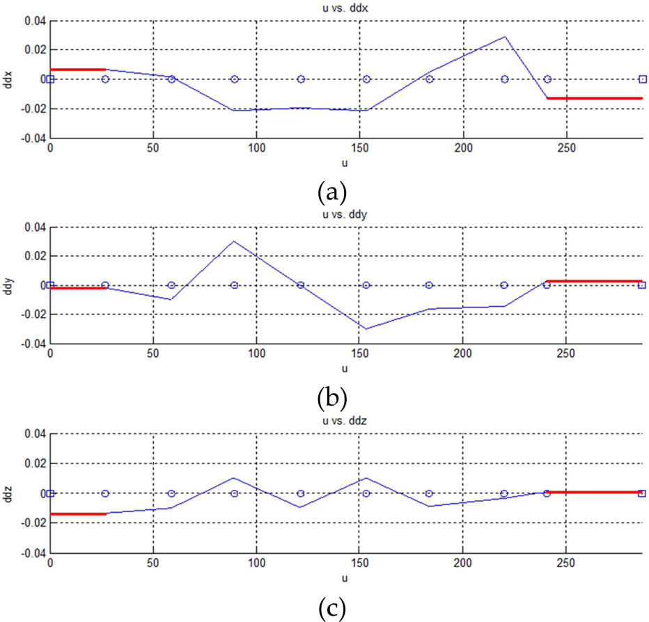
Second-order differential values of the smoothed path: (a) is the x, (b) is the y, and (c) is the z axis

Figure 9.

Graph of curvature

The proposed method does not use trigonometric and high-order functions.

7. Conclusions

Many studies have focused on finding collision-free paths and solving mazes on the 2D plane. However, in real environments, movements are required to be stable. In order to achieve stable movement, paths should be continuous.

For aerial robots and aerial vehicles, the movement must follow a smooth path in the 3D space. They must maintain velocity and cannot change direction rapidly. General waypoint-planning methods form paths only using waypoints without considering the continuity of the path. If aerial robots and aerial vehicles follow a planned continuous path, the flight can be made more stable through optimal movements using the shortest path.

This paper has proposed a method for constructing the 3D smooth path from waypoints in a 3D space. The path must visit every waypoint and have G² continuity. The 3D smooth path is obtained without using complex calculations such as trigonometric functions or using high-order polynomial functions.

The proposed method expands the QPMI path-smoothing method and uses quadratic polynomial interpolation to create the unique, shortest, G² continuous path about three waypoints. This paper takes these advantages of quadratic polynomial interpolation for constructing the 3D smooth path. The proposed method has two steps. The first step is to make waypoint groups that consist in three waypoints. Each group has its own path obtained from the parametric quadratic polynomial interpolation. The 3D path is expressed using a parametric method and is the G² continuous path about each waypoint group having the unique, shortest path. The second step is to combine the planned waypoint group's paths. The membership function uses the parameter u and distributes the degree of each waypoint group's path. Each path is merged into one path to maintain continuity. The planned path is shown to be the G² continuous 3D path.

The proposed 3D path-smoothing method uses only quadratic polynomials and features a relatively simple computation. It produces a unique, shortest, G² continuous path that visits all the waypoints. The curvature of the path is verifiable. This method can also be combined with a waypoint planner or a path-searching method to construct a 3D smooth path. In addition, this method does not require storage for saving path data. These advantages enable the development of a simple system.

8. Acknowledgements

This research was supported by the Inha University.

References

Stentz

, “The focussed D^* algorithm for real-time replanning,” in Artificial Intelligence. International Joint Conference on, pp. 1652–1659, 1995.

Hwang

Y. K.

and Ahuja

, “A potential field approach to path planning,” Robotics and Automation. IEEE Transactions on, vol. 8, pp. 23–32, 1992.

Kavraki

L. E.

Svestka

Latombe

J.-C.

, and Overmars

M. H.

, “Probabilistic roadmaps for path planning in high-dimensional configuration spaces,” Robotics and Automation, IEEE Transactions on, vol. 12, pp. 566–580, 1996.

Kuffner

J. J.

Jr and LaValle

S. M.

, “RRT-connect: An efficient approach to single-query path planning,” in Robotics and Automation (ICRA'00). Proceedings, IEEE International Conference on, pp. 995–1001, 2000.

Hasircioglu

Topcuoglu

H. R.

, and Ermis

, “3D path planning for the navigation of unmanned aerial vehicles by using evolutionary algorithms,” in Genetic and Evolutionary Computation. Proceedings, 10th Annual Conference on, pp. 1499–1506, 2008.

Babaei

and Mortazavi

, “Three-dimensional curvature-constrained trajectory planning based on in-flight waypoints,” Journal of Aircraft, vol. 47, pp. 1391–1398, 2010.

Kim

H. J.

and Shim

D. H.

, “A flight control system for aerial robots: algorithms and experiments,” Control Engineering Practice, vol. 11, pp. 1389–1400, 2003.

Anderson

J. D.

, Fundamentals of Aerodynamics, vol. 2. New York: McGraw-Hill, 2001.

Farin

G. E.

, Curves and surfaces for CAGD: a practical guide. 5th ed. San Francisco, CA, USA: Morgan Kaufmann Publishers Inc., 2002.

10.

Magid

Keren

Rivlin

, and Yavneh

, “Spline-based robot navigation,” in Intelligent Robots and Systems. 2006 IEEE/RSJ International Conference on, pp. 2296–2301, 2006.

11.

Komoriya

and Tanie

, “Trajectory design and control of a wheel-type mobile robot using B-spline curve,” in Intelligent Robots and Systems (IROS'89), The Autonomous Mobile Robots and Its Applications. Proceedings, IEEE/RSJ International Workshop on, pp. 398–405, 1989.

12.

Piazzi

Bianco

C. G. L.

, and Romano

, “Smooth path generation for wheeled mobile robots using <unknown entity>3-splines,” Motion Control, Casolo

Federico

(Ed.), pp. 75–96, 2010.

13.

Berglund

Jonsson

, and Soderkvist

, “An obstacle-avoiding minimum variation b-spline problem,” in Geometric Modeling and Graphics. Proceedings, 2003 International Conference on, pp. 156–161, 2003.

14.

Anderson

E. P.

Beard

R. W.

, and McLain

T. W.

, “Real-time dynamic trajectory smoothing for unmanned air vehicles,” Control Systems Technology, IEEE Transactions on, vol. 13, pp. 471–477, 2005.

15.

Jung

and Tsiotras

, “On-line path generation for small unmanned aerial vehicles using B-spline path templates,” in AIAA Guidance, Navigation and Control Conference, AIAA, vol. 7135, 2008.

16.

Yang

and Sukkarieh

, “3D smooth path planning for a UAV in cluttered natural environments,” in Intelligent Robots and Systems (IROS 2008). IEEE/RSJ International Conference on, pp. 794–800, 2008.

17.

Huh

U. Y.

and Chang

S. R.

, “A G² Continuous Path-smoothing Algorithm Using Modified Quadratic Polynomial Interpolation,” International Journal of Advanced Robotic Systems, vol. 11, p. 25, 2014.

18.

Chang