Sage Journals: Discover world-class research

Abstract

This work is focused on the design, construction and model based control of a biped robot during the walking cycle on the sagittal plane. For the analysis, the single support phase is considered to be the dominating dynamics, by assuming an instantaneous double support phase which is only described by the impact phenomenon. The joint tracking problem is analyzed by means of a model based control strategy, which incorporates a reformulation of the Coriolis matrix that allows the cancellation of non antisymmetric terms in order to formally proof the asymptotic stability of the coordinate error system representation in a local sense. Some experiments are carried out for a pre-defined reference trajectory for the walking cycle of a 4-DOF biped robot.

Keywords

Biped Robot Dynamics Walking Cycle

1. Introduction

It is clear how the legged locomotion systems has had an increasing interest in the last decades; in particular biped robots have gained attention because of their special characteristics regarding their performance on difficult environments. There exists a large variety of works in the literature addressing several approaches of biped locomotion, some of them deal fundamentally with dynamic models; for instance, in [1] and [2] a model of a biped robot is developed and experimentally validated; in [3] it is obtained a dynamic model which is only implemented in a simulation platform; or in [4], the dynamics of the robot is analyzed via systems with impulse effects. Regarding the walking cycle, a typical gait is divided into two phases, the single and the double support [5], [3]; although sometimes it is considered only the single support phase with boundary conditions [2], [4]. In some situations, it is incorporated a third phase [6], which corresponds to a flight phase in a running mode. It is also widely addressed the dynamic walking stability for particular feedback controllers; for example in [7], where it is considered the double support event as a perturbation of the single support dynamics, the stability is analyzed in terms of Lyapunov strategies. The use of Poincare maps and limit cycles has been discussed in [8], [4], [9]. The design of reference trajectories is also an important topic in terms, for example, of optimal performance [5], [10]; natural inspired evolution [11]; or time dependent polynomial design [12]. Additionally, the mechanical design of a biped robot structure has been addressed in order to get special characteristics of mobility; this fact however represents an important energy consumption issue. Many structural designs has been proposed; for instance, in [13] a biped robot is designed with a rickshaw-based mechanism and, in [14], a biped robot is actuated only with one motor by taking advantage of passive characteristics of its structure. In [15], the energy consumption is addressed by means of a special joint and drive mechanism. The use of cables, screw-nut systems, gears and springs have been also widely considered; see for instance [16], [17], [18] and [19].

Concerning control strategies, biped locomotion has been studied with different feedback schemes such as passivity based techniques [20]; adaptive control [21] or sliding mode strategies [22]. In [23], it is presented a dynamic model of a biped robot, and a computed-torque control feedback has been experimentally implemented, taking into account the non-modeled forces on the motor gear on each union. In [24], it is assumed that the mass inertia of the legs is sufficiently small; the design is complemented with a feedback linearization strategy which is experimentally implemented in a physical platform. The classical computed-torque control is also implemented in [25] for a 7-link biped robot by incorporating a gravity compensation scheme.

In this work it is assumed that the biped robot dynamics is totally defined by the single support phase, taking into account the double support as a discontinuous phenomenon, due to the impact of the swing leg with the ground and the swapping of coordinates such that the stance leg becomes the swing leg and vice versa. The control strategy is developed by considering the structural characteristics of the single support phase model and by means of a new representation of the Coriolis matrix. This fact allows to show the asymptotic stability of the error coordinates for the closed-loop system. Also, in the physical platform, the control torque signals are applied by means of screw-nut arrays in order to obtain a low torque demand at the actuators.

The rest of the paper is organized as follows: In Section 2, it is presented a brief description of the considered biped robot and its dynamic model is obtained by an Euler-Lagrange formulation describing also their main structural properties. In Section 3, it is addressed the physical laboratory prototype. It is also stated the mobility characteristics and the type of actuation for each joint. Section 4 describes the design of the feedback control law by taking into account the obtained dynamic model. In this section, a stability analysis is developed by means of a Lyapunov technique. The experimental results for the closed-loop system are presented in Section 5, where the reference trajectory is also defined. Finally, some conclusions are given in Section 6.

2. Class of biped robot

The structure of the biped robot is designed with two degrees of freedom per leg, corresponding to the knee and hip joints. Since torso and ankle are not considered, it is obtained a 4-DOF system. The dynamic analysis is carried out on the sagittal plane with a punctual contact with the ground. In the literature, more complex robot designs have been addressed; however the apparent simplicity of the proposed configuration follows from the attempt to successfully implement, in real time, a particular actuation mechanism with a specific feedback control. The walking cycle is considered as a periodic event defined by a single support phase dynamics, restarted by an instantaneous double support. This restarting phenomenon is described by means of the impact dynamics that produces an instantaneous change on the joint velocities without affecting the robot posture. In addition, it is assumed that the robot does not slip at either the support or the impact point. This fact implies new initial conditions at the beginning of each step. This general control strategy has been implemented following [7].

2.1 Biped robot dynamics

The class of biped robot is depicted in Figure 1.

Figure 1.

Biped robot configuration.

The robot dynamics is obtained by means of the Euler Lagrange formulation [26], under the hypothesis of concentrated mass at each link and the assumption of neglected friction force at joints and actuators. Therefore, the standard representation of the single support phase model is stated as,

D (q (t)) \ddot{q} (t) + C (q (t), \dot{q} (t)) \dot{q} (t) + G (q (t)) = B τ (t),

(1)

where q(t) = [q₃₁(t)q₃₂(t)q₄₁(t)q₄₂(t)]^T is the generalized coordinates vector. As usual, D(q) is the inertia matrix, bounded and positive definite, and C(q,q̇) is the matrix of Coriolis and centripetal forces. G(q) represents a matrix of gravitational effects and B defines the input matrix. The τ(t) = [τ₃₁ (t) τ₃₂ (t) τ₄₁ (t) τ₄₂ (t)]^T defines the applied joint torques of the robot.

After a straightforward computation, matrices D(q),C(q,q̇),G(q) and B involved on the single support model (1), can be defined as,

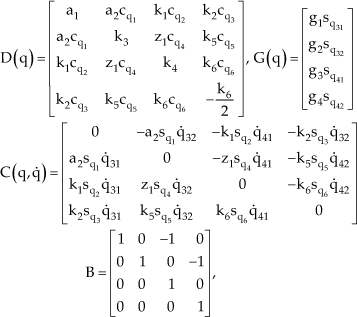
\begin{array}{l} D (q) = [\begin{matrix} a_{1} & a_{2} c_{q_{1}} & k_{1} c_{q_{2}} & k_{2} c_{q_{3}} \\ a_{2} c_{q_{1}} & k_{3} & z_{1} c_{q_{4}} & k_{5} c_{q_{5}} \\ k_{1} c_{q_{2}} & z_{1} c_{q_{4}} & k_{4} & k_{6} c_{q_{6}} \\ k_{2} c_{q_{3}} & k_{5} c_{q_{5}} & k_{6} c_{q_{6}} & - \frac{k_{6}}{2} \end{matrix}], G (q) = [\begin{matrix} g_{1} s_{q_{31}} \\ g_{2} s_{q_{32}} \\ g_{3} s_{q_{41}} \\ g_{4} s_{q_{42}} \end{matrix}] \\ C (q, \dot{q}) = [\begin{matrix} 0 & - a_{2} s_{q_{1}} {\dot{q}}_{32} & - k_{1} s_{q_{2}} {\dot{q}}_{41} & - k_{2} s_{q_{3}} {\dot{q}}_{32} \\ a_{2} s_{q_{1}} {\dot{q}}_{31} & 0 & - z_{1} s_{q_{4}} {\dot{q}}_{41} & - k_{5} s_{q_{5}} {\dot{q}}_{42} \\ k_{1} s_{q_{2}} {\dot{q}}_{31} & z_{1} s_{q_{4}} {\dot{q}}_{32} & 0 & - k_{6} s_{q_{6}} {\dot{q}}_{42} \\ k_{2} s_{q_{3}} {\dot{q}}_{31} & k_{5} s_{q_{5}} {\dot{q}}_{32} & k_{6} s_{q_{6}} {\dot{q}}_{41} & 0 \end{matrix}] \\ B = [\begin{array}{r} 1 & 0 & - 1 & 0 \\ 0 & 1 & 0 & - 1 \\ 0 & 0 & 1 & 0 \\ 0 & 0 & 0 & 1 \end{array}], \end{array}

where, for simplicity of notation, it has been defined s_(·)sin_(·),c_(·)cos(·),and

\begin{array}{l} q_{1} = q_{32} - q_{31}, q_{2} = q_{41} - q_{31}, q_{3} = q_{42} - q_{31} \\ q_{4} = q_{41} - q_{32}, q_{5} = q_{42} - q_{32}, q_{6} = q_{42} - q_{41} . \end{array}

(2)

Beingg the gravity constant, parameters a_i, k_i, z_i and g_i depend on the structural configuration of the robot and they are given in Table 1.

Table 1.

Structural model parameters.

$a_{1} = L \frac{2}{3} (\frac{5}{4} M_{3} + M_{4} + M_{H})$	$k_{1} = L_{4} (\frac{a_{1}}{L_{3}} + L_{3} \frac{1}{4} M_{3})$
$a_{2} = - L \frac{2}{3} (\frac{1}{2} M_{3} + M_{4})$	$k_{2} = - \frac{1}{2} M_{4} L_{3} L_{4}$
$g_{1} = L_{3} g (\frac{3}{2} M_{3} + M_{4} + M_{H})$	$k_{3} = L \frac{2}{3} (\frac{1}{4} M_{3} + M_{4})$
$g_{2} = - L_{3} g (\frac{1}{2} M_{3} + M_{4})$	$k_{4} = L \frac{2}{4} (\frac{5}{4} M_{4} + 2 M_{3} + M_{H})$
$g_{3} = L_{4} g (2 M_{3} + \frac{3}{2} M_{4} + M_{H})$	$k_{5} = \frac{1}{2} M_{4} L_{3} L_{4}$
$g_{4} = - \frac{1}{2} L_{4} M_{4} g$	$k_{6} = - \frac{1}{2} M_{4} L \frac{2}{4}$
z₁₌L₄a₂/L₃

2.1.1 Structural properties.

The biped robot model satisfies the following structural properties that will be used later on the development of the control strategy. Most of them are in accordance with the dynamic model of a general robot manipulator [26].

Property 1. Matrices Ḋ(q) and C(q,q̇) are such that: i) Ḋ(q) – 2C(q,q̇) = N(q,q̇) for a skew symmetric matrix N(q,q̇) and ii) Ḋ(q)-C(q,q̇) = C^T(q,q̇).

Property 2. For any vectors z,w ∈ Rⁿ: i) C(q,q̇) w = C(q,w)q̇ and ii) C(q,z + w) =C(q,z) +C(q,w).

Property 3. C(q,q̇) is a bounded matrix, i.e. ‖C(q,q̇)| ≤ k‖q̇‖ for some k ∈ R.

In addition, the Coriolis matrix satisfies the following property, which is very useful in the synthesis of the feedback control.

Property 4. Matrix C(q,q̇) can be rewritten in terms of a skew-symmetric matrix C₁(q,q̇) as C(q,q̇) = C₁(q,q̇)+C₂(q,q̇) with,

\begin{array}{l} C_{1} = [\begin{matrix} 0 & - a_{2} s_{q_{1}} {\dot{q}}_{31} & - k_{1} s_{q_{2}} {\dot{q}}_{31} & - k_{2} s_{q_{3}} {\dot{q}}_{31} \\ a_{2} s_{q_{1}} {\dot{q}}_{31} & 0 & - z_{1} s_{q_{4}} {\dot{q}}_{32} & - k_{5} s_{q_{5}} {\dot{q}}_{32} \\ k_{1} s_{q_{2}} {\dot{q}}_{31} & z_{1} s_{q_{4}} {\dot{q}}_{32} & 0 & - k_{6} s_{q_{6}} {\dot{q}}_{41} \\ k_{2} s_{q_{3}} {\dot{q}}_{31} & k_{5} s_{q_{5}} {\dot{q}}_{32} & k_{6} s_{q_{6}} {\dot{q}}_{41} & 0 \end{matrix}] \\ a n d \\ C_{2} = [\begin{matrix} 0 & - a_{2} s_{q_{1}} {\dot{q}}_{1} & - k_{1} s_{q_{2}} {\dot{q}}_{2} & - k_{2} s_{q_{3}} {\dot{q}}_{3} \\ 0 & 0 & - z_{1} s_{q_{4}} {\dot{q}}_{4} & - k_{5} s_{q_{5}} {\dot{q}}_{5} \\ 0 & 0 & 0 & - k_{6} s_{q_{6}} {\dot{q}}_{6} \\ 0 & 0 & 0 & 0 \end{matrix}] . \end{array}

To complete the walking cycle, the double support phase is defined in terms of an instantaneous impact dynamics and a swapping strategy, producing a set of initial conditions for the next step. With this aim, it is assumed that the impact with the ground of the current swing leg, at the end of each step, produces an instantaneous change of the joint velocities without implying a change in the posture of the robot. This approach has been widely considered in the literature; see for instance [4] and [27].

For the analysis of the double support phase, it has been considered two additional coordinates, [ζ₁, ζ₂]^T to define the Cartesian position of the end-point of the stance leg in the X–Y plane. In this way, an extended vector of generalized coordinates q_e = [q₃₁ q₃₂ q₄₁ q₄₂ ζ₁ ζ₂]^T is also defined.

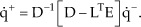
In order to obtain an analytical expression for the velocity just after the impact q̇⁺, consider the kinetic energy of the robot from the extended model as,

T = \frac{1}{2} {\dot{q}}_{e}^{T} D_{e} (q_{e}) {\dot{q}}_{e}

(3)

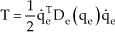
where the extended inertia matrix D_e has the form,

D_{e} (q_{e}) = [\begin{matrix} D (q) & L {(q)}^{T} \\ L (q) & M \end{matrix}]

(4)

with D(q) being the original inertia matrix of (1) and,

L (q) = [\begin{matrix} b_{1} c_{31} & b_{2} c_{32} & b_{3} c_{41} & b_{4} c_{42} \\ b_{1} s_{31} & b_{2} s_{32} & b_{3} s_{41} & b_{4} s_{42} \end{matrix}]

with,

\begin{array}{l} b_{1} = L_{3} (\frac{3}{2} M_{3} + M_{4} + M_{H}), b_{2} = - L_{3} (\frac{1}{2} M_{3} + M_{4}) \\ b_{3} = L_{4} (\frac{3}{2} M_{4} + 2 M_{3} + M_{H}), b_{4} = - \frac{1}{2} M_{4} L_{4} \end{array}

and

M = [\begin{matrix} 2 M_{4} + 2 M_{3} + M_{H} & 0 \\ 0 & 2 M_{4} + 2 M_{3} + M_{H} \end{matrix}] .

Substituting Equation (3) into the Lagrange's impulsive equation as in [28], yields,

D (q) {\dot{q}}^{+} - D (q) {\dot{q}}^{-} - L {(q)}^{T} [\begin{matrix} {\dot{x}}_{2} \\ {\dot{y}}_{2} \end{matrix}] = 0,

(5)

where q̇^– is the articular velocity just before the impact and [x₂y₂]^T is the position of the end-point of the swing leg with respect to the supporting point. Moreover, the slipping relation at the end of the impact leg is expressed as,

[\begin{matrix} {\dot{x}}_{2} \\ {\dot{y}}_{2} \end{matrix}] = E {\dot{q}}^{-}

(6)

where E is the Jacobian defined as,

E = \frac{\partial P_{2}}{\partial q}

(7)

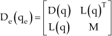
with P₂= [x₂y₂]^T. The post impact velocities q̇+ can be expressed from (5) and (6) as,

{\dot{q}}^{+} = D^{- 1} [D - L^{T} E] {\dot{q}}^{-} .

(8)

Notice that, since matrices D and L^TE are bounded, the post impact velocity does not increase indefinitely.

Once the post impact articular velocities are known, the supporting and swing leg swapping is defined by the map,

[\begin{matrix} q^{+} \\ q^{+} \end{matrix}] = R [\begin{matrix} q^{-} \\ D^{- 1} [D - L^{T} E] {\dot{q}}^{-} \end{matrix}]

(9)

where R is a transformation matrix defined as,

R = [\begin{array}{l} T & 0_{n \times n} \\ 0_{n \times n} & T \end{array}]

with

T = [\begin{matrix} 0 & 1 & 0 & 0 \\ 1 & 0 & 0 & 0 \\ 0 & 0 & 0 & 1 \\ 0 & 0 & 1 & 0 \end{matrix}] .

The described velocity discontinuities and the defined boundedness characteristic, which can be stated with a particular reference, allow to consider the double support as a perturbation of the states in the single support model.

3. Physical platform

The biped robot has been designed in order to be dynamically analyzed only on the sagittal plane. To carry out the experiments, an external restricting frame has been designed by means of a translational free movement mechanism along the vertical and horizontal axes. This exostructure avoids the robot to fall down on the lateral plane and provides a free movement on the forward direction. The robot is fixed to the exostructure at the hip, allowing a simple noninvasive support. Figure 2 shows this structural frame. Notice that, apparently, there is an element that acts as a torso; however, it is not free to rotate and its dynamics is neglected.

Figure 2.

Physical platform.

The robot is built with a particular actuator mechanism at each joint which allows to generate the high torque requirements from a low torque actuator; however it has an important drawback that relies on a high velocity demand. The design is based on [17] and consists basically on a linkage mechanism, where the main input is provided by a brushed DC motor, producing a translational movement along a ball bearing screw, converting in this way the rotational movement into a translational one. Complementary, the linkage mechanism produces the required rotational movement for the knee and hip joints. This mechanical interface is depicted in Figure 3 for the hip (right) and the knee (left) joints.

Figure 3.

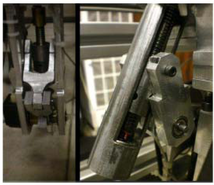
Detail of the linkage mechanism.

In Figure 4, a schematic diagram is presented with this concept.

Figure 4.

Schematic representation of the knee and hip joints.

The analysis of the proposed mechanism can be developed in terms of the dimensional parameters (Figure 4) and the dynamics of a screw. Basically, and based on [17], kinematic relations allow to define the velocity of the nut of the screw with respect to a desired reference and as a function of the motor velocity. For instance, from Figure 4, it can be obtained the vertical position of the nut in the knee (left side), which after a time derivation can be expressed as,

- L_{m k} [s e n (π - q_{k} - ϑ) + \frac{a_{k}}{b_{k}} c o s (π - q_{k} - ϑ)] {\dot{q}}_{k} = \frac{p}{2 π} {\dot{q}}_{m k}

(10)

where q_k = q_4w, w = 1, 2; denotes a general knee coordinate and q̇_mk is the velocity of the corresponding knee motor. Equation (10) allows to obtain a relation between the motor and joint velocities of the form q̇_mk=ξ_k(q_k)q̇_k with a gain factor for the knee ξ_k(q_k) given as,

ξ_{k} (q_{k}) = - \frac{2 π L_{m k}}{p} [s e n (π - q_{k} - ϑ) + \frac{a_{k}}{b_{k}} c o s (π - q_{k} - ϑ)] .

(11)

Equivalently, a gain factor for the hip ξ_h(q_h) is obtained as,

ξ_{h} (q_{h}) = - \frac{2 π L_{m h}}{p} [c o s (π - q_{h} + α) + \frac{a_{h}}{b_{h}} s i n (π - q_{h} + α)]

(12)

with q_h=q_3w,w = 1, 2, describing the general hip coordinate. In both cases, it is defined,

\begin{array}{l} a_{h} = d_{d i a g} - L_{m c} c o s (π - q_{h} + α) \\ b_{h} = \sqrt{L_{b h}^{2} - a_{h}^{2}} \\ a_{k} = L_{m k} s i n (π - q_{k} - ϑ) + d_{h o r} \\ b_{k} = \sqrt{L_{b k} - a_{k}^{2}} . \end{array}

Notice that the parameters from Equations (11) and (12) describe physical dimensions; therefore they rely on the dimensions of the physical platform that has been previously designed and constructed in order to satisfy velocity and torque requirements. These parameters are numerically expressed in Table 2.

Table 2.

Physical parameters.

L_mk = 0.04m	d_diag = 0.06m	M_T = 6Kg	$q_{h_{m i n}} = 160^{o}$
L_bk = 0.06m	ϑ = 0.26rad	M_h = 2.30Kg	$q_{h_{m a x}} = 220^{o}$
L_mc = 0.04m	η = 0.85	M₃ = 1.20Kg	$q_{k_{m i n}} = 110^{o}$
L_bc = 0.03m	d_hor = 0.02m	M₄ = 0.32Kg	$q_{k_{m a x}} = 160^{o}$
α = 0.50rad	screw = 0.1m	p = 0.002m

The mechanical advantage of the linkage mechanism is determined by the gains factors (11) and (12) for the articular range of each joint. Those factors describe the torque gain at each joint from the motor and, at the same time, the corresponding velocity relation. Figures 5a and 6a, show how the required torque at each joint is reflected in a quite low torque in the corresponding DC motor. Also, it is possible to see how the velocity at the motor is increased (Figures 5b and 6b) in order to satisfy a particular reference trajectory. The performance of the linkage mechanism is evaluated as a linear displacement of the nut along the screw, which implies a continuous angular motion at each joint. For this particular situation, Figure 5a shows how a high torque of 80Nm at the hip joint is reduced at the motor shaft to 1.5Nm, assuring an adequate behavior of the mechanism. An inverse effect can be seen from Figure 5b with respect to velocities. A similar analysis can be also obtained for the knee from Figure 6b. The input-output torque and velocity relations can be manipulated by changing the involved mechanical parameters.

Figure 5.

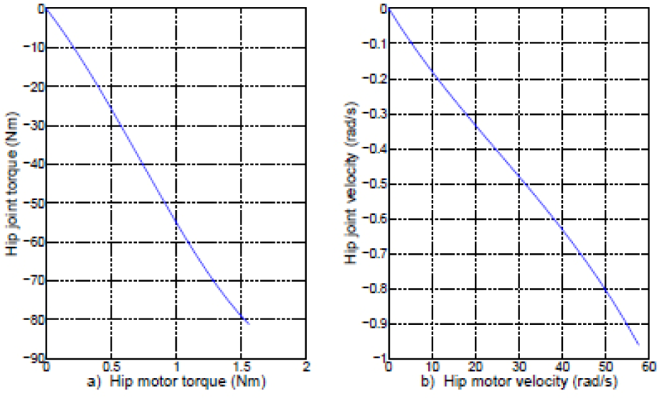
Hip torque and velocity rate.

Figure 6.

Knee torque and velocity rate.

The proposed mechanical interface implies a working space that is delimited by the total displacement of the nut along the screw, as well as the length of the involved elements. This characteristic defines displacement restrictions at each joint which in general can be described as,

q_{h_{m i n}} \leq q_{h} \leq q_{h_{m a x}}

(13)

q_{h_{m i n}} - π + q_{k_{m i n}} \leq q_{k} \leq q_{h_{m a x}} - π + q_{k_{m a x}}

(14)

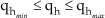
where q_h and q_k are the hip and knee joint angles respectively. The working ranges are defined with respect to an absolute vertical reference as defined in Figure 1.

However the limits $q_{h_{m i n}}, q_{h_{m a x}}, q_{k_{m i n}}$ and $q_{k_{m a x}}$ are defined in a local reference frame, this is, the femur is measured with respect to the hip and the tibia with respect to the femur. These relations are depicted in Figure 7 and their numerical values are specified in Table 2.

Figure 7.

Mechanical limits for the legs.

As stated, the contact with the walking surface is designed to be punctual and a pressure mechanism consisting of a low cost resistive sensor has been implemented at the end of each leg such that the induced pressure force at this point can be measured. In this particular case, the force is used to detect the impact instant and its magnitude is not relevant. This implementation is depicted in Figure 8.

Figure 8.

Pressure mechanism at the end of each leg.

To compute the articular position, an optical encoder is installed at each joint. Also, there is an inclinometer at each tibia to sense an eventual fall of the mechanism. Limit switches are used to prevent a mechanical damage as a consequence of displacements out of the ranges previously described.

It is clear that the complexity of the mechanical prototype is not totally described by the mathematical model (1) due to (among others) the fact that this model does not consider the auto-lock characteristic that the type of actuation induces, this is, the model assumes that the motor acts directly at the joint. However, it is possible to incorporate the effects of the actuation mechanism by means of the relation,

τ = ξ_{j} (q) τ_{m}

(15)

where τ_m is the motor torque; the subscript j defines the hip joint, j = h, or the knee joint, j = k; and τ is the control signal for each joint. Notice that ξ_j(q) are defined in Equations (11) y (12) and they have an inverse role when acting as gain factors with torque signals.

4. Model based control strategy

In this section it is addressed the proposed control strategy in order to get a stable walking cycle. Roughly speaking a global asymptotic stability is not possible because of the nature of the complete walking cycle in terms of a resetting event at each end of step; however, the assumption of considering the single support phase as the main dynamics, allows to locally analyze the walking cycle as a perturbed dynamics with a periodic perturbation described by an instantaneous double support. This approach has been already studied in [7].

Taking into account model (1), it can be proposed a model-based feedback control as,

\begin{array}{l} B ξ_{j} (q) τ_{m} = D (q) {\ddot{q}}_{d} + C (q, {\dot{q}}_{d}) {\dot{q}}_{d} + G (q) \\ - k_{d} \dot{\overset{..}{q}} - k_{p} \overset{..}{q} + C_{2} (q, {\dot{q}}_{d}) \dot{\overset{..}{q}} \end{array}

(16)

where k_d ∈ R^n×n and k_p ∈ R^n×n are diagonal positive definite matrices and q˜ = q–q_d is the joint tracking error with q_d representing a sufficiently smooth desired joint trajectory.C₂(q,q̇_d) is an upper triangular matrix previously defined in Property 4.

Notice that Equation (16) is defined in the joint space; however, the absolute reference and the real dynamics are first expressed in the Cartesian plane. In this way, a desired Cartesian performance is indirectly induced by means of an expected stable feedback control through an inverse kinematic mapping.

In addition, the term ξ_j(q) results in a scalar that is assigned with a suitable transformation such that it matches with the corresponding joint, either hip or knee. Moreover, it is required that ξ_j(q) ≠ 0, which means that,

q_{h} \neq a t a n (\frac{b_{h}}{a_{h}}) + π + α

(17)

and

q_{k} \neq a t a n (\frac{a_{h}}{b_{h}}) + π - ϑ,

(18)

hence, the definition of the desired performance has to consider this fact.

Finally, notice that matrix B is invertible, so the calculation of the motor torques is directly obtained from Equation (16) in a practical implementation.

Lemma 5. Consider system (1) and the feedback law given in equation (16). Under these conditions, feedback (16) renders the closed-loop system (1)–(16) asymptotically stable.

Proof. The closed-loop system (1)–(16) results in,

D (q) \ddot{\overset{..}{q}} + C (q, \dot{q}) \dot{q} - C (q, {\dot{q}}_{d}) {\dot{q}}_{d} + [k_{d} - C_{2} (q, {\dot{q}}_{d})] \dot{\overset{..}{q}} + k_{p} \overset{..}{q} = 0.

(19)

Notice that, by considering Property 2,

C (q, \dot{q}) \dot{q} - C (q, {\dot{q}}_{d}) {\dot{q}}_{d} = [C (q, \dot{q}) + C (q, {\dot{q}}_{d})] \dot{\overset{..}{q}} .

Then, Equation (19) can be written as,

D (q) \ddot{\overset{..}{q}} + [C (q, \dot{q}) + C (q, {\dot{q}}_{d})] \dot{\overset{..}{q}} + k_{d} \dot{\overset{..}{q}} + k_{p} \overset{..}{q} - C_{2} (q, {\dot{q}}_{d}) \dot{\overset{..}{q}} = 0.

(20)

The latter equation allows to show the importance of Property 4, which helps to finally obtain the closed–loop dynamic as,

D (q) \ddot{\overset{..}{q}} + [C (q, \dot{q}) + C_{1} (q, {\dot{q}}_{d}) + k_{d}] \dot{\overset{..}{q}} + k_{p} \overset{..}{q} = 0.

(21)

Noting first that the error dynamics given by Equation (21) has an equilibrium point at the origin, $(\dot{\overset{..}{q}}, \overset{..}{q}) = (0, 0),$ , the closed-loop stability analysis can be done by considering a Lyapunov candidate function of the form,

V (\overset{..}{q}, \dot{\overset{..}{q}}) = \frac{1}{2} {\dot{\overset{..}{q}}}^{T} D \dot{\overset{..}{q}} + \frac{1}{2} {\overset{..}{q}}^{T} k_{p} \overset{..}{q} .

(22)

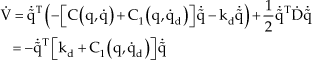
The time derivative of $V (\overset{..}{q}, \dot{\overset{..}{q}})$ along the solution of (21) produces,

\begin{array}{l} \dot{V} = {\dot{\overset{..}{q}}}^{T} (- [C (q, \dot{q}) + C_{1} (q, {\dot{q}}_{d})] \dot{\overset{..}{q}} - k_{d} \dot{\overset{..}{q}}) + \frac{1}{2} {\dot{\overset{..}{q}}}^{T} \dot{D} \dot{\overset{..}{q}} \\ = - {\dot{\overset{..}{q}}}^{T} [k_{d} + C_{1} (q, {\dot{q}}_{d})] \dot{\overset{..}{q}} \end{array}

and the fact that C₁(q,q̇_d) is a skew-symmetric matrix according to Property 4, allows to finally obtain,

\dot{V} (\overset{..}{q}, \dot{\overset{..}{q}}) = - {\dot{\overset{..}{q}}}^{T} k_{d} \dot{\overset{..}{q}} .

It is now clear that by considering the LaSalle's invariance principle; it is possible to show the required asymptotic stability for the error coordinate q˜.

It is evident that the above lemma holds only when the single support phase is defined as the main dynamics. This means that, in a complete analysis of the walking cycle, the effect of the impact avoids to obtain an asymptotic stability property, because of the expected and periodic discontinuity of the error coordinates. In order to overcome this problem, a possible solution could be the definition of a reference path profile that includes the impact dynamics described by Equation (9) at the end of the step. However, this is not practical because of the switching reference requirement that in general does not allow to produce a perfect tracking and the asymptotic property does not even hold.

The approach that has been considered in this work consists on the definition of a reference trajectory such that at the impact, the velocities are sufficiently low and the impulse effects are not significant. Even with the adopted approach, the asymptotic stability cannot be stated, fulfilling only a simple condition of stability. In order to analyze the impact into the complete walking cycle, a natural approach corresponds to a hybrid system that involves impulse effects; studied in [4] for biped robots.

It is important to clarify that the above result is a theoretical one. This means that in order to guarantee dynamical stability, the robot has to perfectly follow the proposed reference. In practice, and due to non modeled dynamics or external disturbances, it is almost impossible to achieve; moreover, the robot could naturally tend to fall when its posture is such that the center of mass CM does not remain exactly over the vertical line defined by the supporting point. This fact could allow to define a non falling condition, just by assuring an immediate support with the swing leg, this is,

x_{2} > | C M_{x} | when | C M_{x} | > 0,

(23)

which means that, when the center of mass CM is out of the vertical line defined by the supporting point, the swing leg should act as an eventual support if the robot tends to fall. This could be similar to a dynamical stability index for robots with superficial contact with the ground, where the non falling condition is assuring by means of a ZMP condition.

5. Real-time evaluation

5.1 Reference Trajectory

The reference trajectory is designed in the Cartesian space and translated to the articular one, where the feedback control is implemented, via inverse kinematics. The trajectory is designed taking into account two points on the robot: the hip and the end point of the swing leg.

It is required that the hip follows a constant reference h_h along the vertical axis Y and, a reference around the origin on the X axis; this latter condition is in order to maintain the center of mass of the robot around the origin during the first part of the step for stability purposes. At the end of step, the center of mass is moved forward on the X axis as a consequence of the passive dynamics produced by the effect of the swing leg when it almost touch the ground.

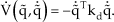
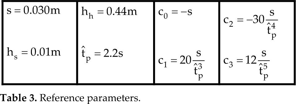
In addition, the trajectory of the end point (x₂, y₂) of the swing leg defines the length of the step and the maximal elevation of the foot. This trajectory is defined by a time dependent, smooth polynomial function of the form,

x_{2} (\hat{t}) = c_{0} + c_{1} {\hat{t}}^{3} + c_{2} {\hat{t}}^{4} + c_{3} {\hat{t}}^{5} .

(24)

For the vertical displacement, the trajectory is designed with a maximal height h_s and a step length s as,

y_{2} (\hat{t}) = h_{s} - \frac{h_{s}}{s^{2}} x_{2}^{2} (\hat{t}) .

(25)

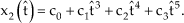
Notice that the vertical trajectory is a function of the horizontal one. Also, the use of the high order polynomial (24) allows to obtain a sufficiently smooth desired trajectory that could reduce the velocity discontinuity at the impact point. Time t̂ is restarted periodically in order to re-define (24) and (25) for the beginning of each step. Table 3 shows the required parameters involved in the reference trajectory functions.

Table 3.

Reference parameters.

s = 0.030m	h_h = 0.44m	c₀ = -s	$c_{2} = - 30 \frac{s}{{\hat{t}}_{p}^{4}}$
h_s = 0.01m	t̂_p = 2.2s	$c_{1} = 20 \frac{s}{{\hat{t}}_{p}^{3}}$	$c_{3} = 12 \frac{s}{{\hat{t}}_{p}^{5}}$

t̂_p is the initial reference time of the step duration, which allows to calculate the coefficients c_i in (24) by means of the interpolation of a specific desired performance; however it does not necessary implies that each step takes exactly this time since the real time duration is determined by the contact of the swing leg with the ground, which eventually could be slightly larger or shorter than t̂_p. This phenomenon defines a new time parameter which is used on the online computation of the new coefficients c_i. Symbolically, those coefficients are defined as in the Table 3.

5.2 Experimental results

To carry out the experiments, feedback law (16) is implemented in a Matlab-Simulink platform, by means of a DSP system DS1104 from Dspace. This board acts as real time interface for the overall system: 1000 cpr optical encoders; two FlexiForce resistive force sensors; two 9000cpr inclinometers at each tibia and the limit switches. Also, the DSP system computes the required feedback law and provides the analog output torque signal for driving the DC motors. A general scheme of the experimental platform is depicted in Figure 9. For all the experiments it was considered a sampling time of 0.001 seconds.

Figure 9.

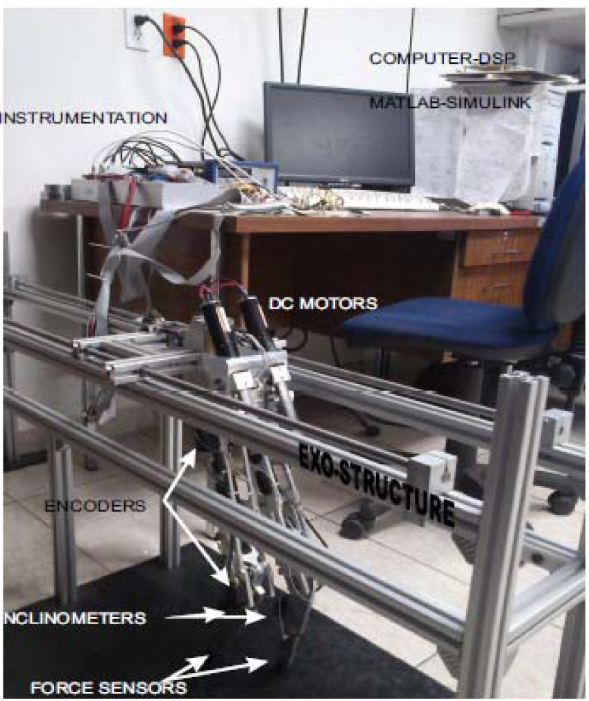
Experimental platform.

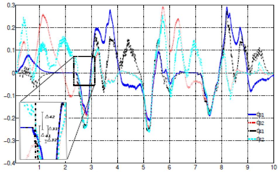
In the experiments, the robot is attempted to follow the reference trajectory previously described which produces the stable dynamical performance of the walking cycle. In Figure 10 it is shown the evolution of the joint coordinates as a result of the robot displacement. This figure depicts the first 10 seconds of the experiment where the robot develops four complete steps divided by dashed vertical lines. As expected, a periodic performance is evident and the feedback control shows a stable result.

Figure 10.

Articular performance of the biped robot.

The corresponding joint velocities are shown in Figure 11; notice that at the end of each step it is possible to appreciate a discontinuity velocity of small magnitude due to the effect of the impact phenomenon. The obtained velocity change is small due to the particular design of the reference trajectory in accordance with the theoretical result.

Figure 11.

Joint velocities of the biped robot.

The evolution of the center of mass in the Cartesian space is depicted in Figure 12. Notice that its position remains around the origin in the horizontal axis as required, being this fact more evident at the beginning of the step. The center of mass is moved forward when the time increases in order to take advantage of the passive characteristic of the robot and finally the step ends.

Figure 12.

Position of the center of mass.

The two Cartesian components of the end point of the swing leg(x₂, y₂) are shown in Figure 13 and the evolution of the hip point (x_H,y_H) is depicted in Figure 14. Notice that the swing leg develops steps with amplitude of 6 cm as required, with a maximal elevation of 1cm from the surface. The hip has a quasi constant evolution in the vertical axis, similar to the center of mass of the robot; however, in the horizontal axis the hip evolves around the origin. This is because the hip element concentrates a larger mass with respect to the rest of the elements and its position is critical for stability purposes.

Figure 13.

Evolution of the end point of the swing leg.

Figure 14.

Position of the hip.

The joint position errors derived from the experiment are shown in Figure 15. Notice that their maximal values appear at the beginning of each step and they decrease with time to a neighborhood of the origin at the end of the step. The performance is apparently erratic and the zero error is not completely attained, this is because the design of the reference trajectory does not directly consider the passive characteristic of the robot, which appears at the end of the step and produce a slight deviation from the expected reference. In spite of this fact, the performance is quite acceptable to satisfy the stable walking cycle.

Figure 15.

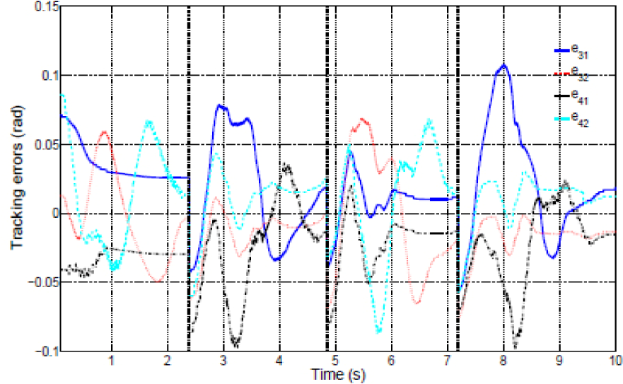
Tracking errors.

The control torque signal at each DC motor shaft is shown in Figure 16 and, in order to show the role of the actuation mechanism, in Figure 17, the torque applied at each joint is also shown.

Figure 16.

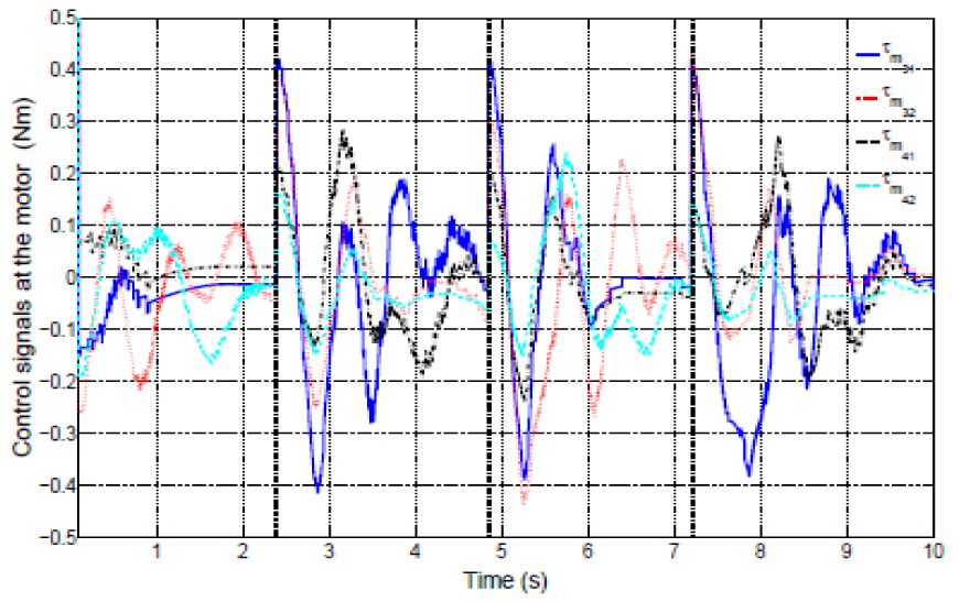
Control signal at the motors.

Figure 17.

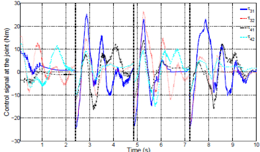
Control signal at the joints.

Notice that there exists a high gain factor from the output torque of each motor, as defined in (11) and (12). It has to be clear that the refered gain factors depend on the performed trajectory in a nonlinear way and they are not totally achieved in the current experiment, where a maximal gain is around 60. However it can be increased by modifying the posture of the robot, taking into account that the velocity will decrease in a proportional rate.

It is important to state that each DC motor has a power supply of 24V, and during the experiments, there exists a maximal current consumption of 1.6 Amperes per motor. It is natural that the maximal consumption is produced by the supporting knee motor, which loads almost all the system when developing a step. In contrast to this situation, the free knee motor consumes no more than 0.2A. In general, it is obtained an average consumption of 2.5A during a single walking cycle which represent no more than 70W of electrical power in total.

6. Conclusions

In this work it is presented the analysis and control of a 4-DOF biped robot. It is considered a particular actuator mechanism with a mechanical advantage which allows to apply high torques on the articulations from a quite small torque at the utilized low power DC motors. The walking cycle is controlled by considering a model based control strategy which is implemented on the single support phase. The double support phase is considered as a perturbation for the robot, producing a change in joint velocities due to the instantaneous impact of the swing leg with the ground; however, in order to minimize their effects, a smooth impact is designed by means of a suitable reference trajectory. It is shown that for the considered feedback, the resulting closed-loop systems is stable. The evolution of the overall control strategy is evaluated on a laboratory prototype showing an adequate performance.

References

Kajita

Yamaura

, and Kobayashi

Dynamic walking control of a biped robot along a potential energy conserving orbits. IEEE Transactions on Robotics and Automation, 8(4):431–438, 1992.

Miura

and Shimoyama

Dynamic walk of a biped. International Journal of Robotics Research, 3(2):60–74, 1984.

Katoh

and Mori

Control method of biped locomotion giving asymptotic stability of trajectory. Automatica, 20(4):405–414, 1984.

Grizzle

J. W.

Abba

, and Plestan

Asymptotically stable walking for biped robots: Analysis via systems with impulse effects. IEEE Transactions on Automatic Control, 46(1):51–64, 2001.

Djoudi

Chevallereau

, and Aoustin

Optimal reference motions for walking of a biped robot. In IEEE International Conference on Robotics and Automation, pages 2002–2007, Barcelona, Spain, 2005.

Chevallereau

and Sardain

Design and actuation optimization of a 4 axes biped robot for walking running. In IEEE International Conference on Robotics ans Automation, pages 3365–3370, San Francisco, CA, USA, 2000.

Chemori

and Loria

Control of a planar five link under-actuated biped robot on a complete walking cycle. In IEEE Conference on Decision and Control, pages 2056–2061, Las Vegas, Nevada, USA, 2002.

Goswami

Ambarish

Espiau

Bernard

, and Keramane

Ahmed

. Limit cycles in a passive compass gait biped and passivity mimicking control laws. Autonomous robots, Springer Netherlands, 4(3):273–286, September 1997.

Plestan

Grizzle

J. W.

Westervelt

E.R

, and Abba

Controlled periodic motion in a nonlinear system with impulse effects: walking of a biped robot. In IFAC NOLCOS-2001, Saint-Petersburg, Russia, 2001.

10.

Xiang

Arora

J.S.

, and Abdel-Malek

Physics-based modeling and simulation of human walking: a review of optimization-based and other approaches. Structural and Multidisciplinary Optimization, 42:1–23, 2010.

11.

France

Girault

, and Espiau

Generation of walk transient trajectories for a biped robot. In International Conference on Advanced Robotics, Tokyo, Japan, October 1999.

12.

Tang

Zhou

, and Sun

Trajectory planning for smooth transition of a biped robot. In Proceedings of IEEE International Conference on Robotics and Automation, pages 2455–2560, 2003.

13.

Ottaviano

Grande

, and Ceccarelli

A biped walking mechanism for a rickshaw robot. Mechanism Based Design of Structures and Machines, 38(2):227–242, 2010.

14.

Berenguer

F.J.

and Monasterio-Huelin

Easy design and construction of a biped walking mechanism with low power consumption. In Proceedings of the 9th International Conference on Climbing and Walking Robots, pages 96–103, Brussels, Belgium, 2006.

15.

Okada

Shinohara

Gotoh

Ban

, and Nakamura

Humanoid robot mechanisms for responsive mobility. In Proceedings of the 2nd International Symposium on Adaptive Motion of Animals and Machines, pages SaP–III–3, 2003.

16.

Constantin

Olaru I. M.

Krut

, and Pierrot

Novel mechanical design of biped robot sherpa using 2 dof cable differential modular joints. In The 2009 IEEE/RSJ International Conference on Intelligent Robots and Systems, pages 4463–4468, St. Louis, USA, 2009.

17.

Sardain

Rostami

, and Bessonnet

An anthropomorphic biped robot: Dynamic concepts and technological design. IEEE Transactions on Systems, Man and Cybernetics-Part A: Systems and Humans, 28(6):823–838, 1998.

18.

Pratap

Singh S.

Dutta

, and Saxena

Design of a biped robot with torsion springs at the joints for reduced energy consumption during walk. In Proceedings of the ASME 2009 International Engineering Technical Conference - Computers and Information in Engineering Conference, 2009.

19.

Yamaguchi

Nishino

, and Takanishi

Realization of dynamic biped walking varying joint stiffness using antagonistic driven joints. In Proceedings of the 1998 IEEE International Conference on Robotics and Automation, pages 2022–2029, Leuven, Belgium, 1998.

20.

Spong

M.W.

Passivity based control of the compass gait biped. In IFAC Triennial Worl Congress, pages 19–23, Beijin, China, 1999.

21.

Vempaty

P. K.

Cheok

K.C.

, and Loh

R. N. L. K.

Model reference adaptive control for actuators of a biped robot locomotion. In Proceedings of the World Congress on Engineering and Computer Science, pages 983–988, San Francisco, USA, 2009.

22.

Tzafestas

Raibert

, and Tzafestas

Robust sliding-mode control applied to a 5-link biped robot. Journal of Intelligent and Robotic Systems, 15(1):67–133, 1996.

23.

Chaillet

Abba

, and Ostertag

Double dynamic modeling and computed-torque control of a biped robot. In IEEE/RSJ Int. Conf. Intelligent Robotics Systems, pages 1149–1153, Munich, Germany, 1994.

24.

Mitobe

Mori

Aida

, and Nasu

Nonlinear feedback control of a biped walking robot. In IEEE International Conference on Robotics and Automation, pages 2865–2870, Nagoya, Japan, 1995.

25.

Park

J. H.

and Kim

K. D.

Biped robot walking using gravity-compensated inverted pendulum mode and computed torque control. In IEEE International Conference on Robotics and Automation, pages 3528–3533, Leuven, Belgium, 1998.

26.

Spong

Mark W.

and Vidyasagar

Robot Dynamics and Control. John Wiler and Sons, USA, 1989.

27.