A Study on Stability of Limit Cycle Walking Model with Feet: Parameter Study

Abstract

In this paper, two kinds of feet, namely, curved and flat feet, are added to limit cycle walking model to investigate its stability properties. Although both models are already proposed and are investigated, most previous works are focused on efficiency and gait behaviors. Only the stability properties of the simplest walking model conceived Garcia et al. are well defined. Therefore, there is still a need for a precise research on the effect of feet, especially in the view of local stability, bifurcation route to chaos, global stability, falling boundary and energy balance line. Therefore, this article revisits the stability analysis of limit cycle walking model with various foot shape. To analyze the effects of feet, we re-derive the equation of motion of modified models by adding one more parameter of foot shape than the simplest walking model. Also, the falling boundary and energy balance line of modified models are derived to get proper initial conditions for stable walking and to explain global stability. Simulation results show us that the curved feet can enlarge both stable walking range and area of basin of attraction while the case of flat feet depends on foot shape parameter.

1. Introduction

Recently, many kinds of biped robots have been developed. Most biped robots are controlled based on ZMP paradigm, despite another paradigm for design and control of biped robots has been studied. In the early 1990s, Tad McGeer proposed passive dynamic walking model which can walk down a gentle slope without any controller except gravity as an energy source [1]. Since then, many research have been conducted in the domain of human waking and biped robots based on passive dynamic walking. Recently passive dynamic walking concept applies not only on a slope but also on a ground using some kinds of actuating strategies [2–3]. The concept including passive dynamic walking alone and with actuating is so called limit cycle walking lately [4]. Biped robots based on limit cycle walking paradigm commonly need less energy than other bipeds and generate pretty natural gait. In order to increase performance and to realize a practical biped, the model needs further studies on its stability, disturbance rejection capability, and versatility, the ability to perform various gaits, etc.

Limit cycle walking models have been studied and demonstrated with simulations and experiments by many researchers, from simple to complex. Goswami et al. studied a compass gait model which has point masses at the hip and on each leg [5]. They studied the dynamics of the model and showed that, depending on the structural parameters of the system, namely, the slope angle, the mass ratio and the length ratio of each leg, passive compass gait may exhibit chaotic gaits, proceeding from cascade of period-doubling bifurcation. Garcia et al. conceived the simplest walking model that has only one free parameter, the slope angle [6]. They studied the behavior of the model analytically and discussed the chaotic gaits with respect to the slope angle. Both models have point feet and are studied in the view of local stability and bifurcation route to chaos according to the slope angle. Wisse et al. studied global stability of Garcia's model using cell-to-cell mapping method [7]. They measured the size of basin of attraction and showed there is no direct relation between the stability of the local stability and global stability. Wisse et al. also studied the effect of upper body, the rule for preventing falling forward and the method to compensate for the yaw and roll motion of a 3D model [8–9]. Ning et al. studied the gait of the model with curved feet model through simulations and experiments [10]. Three parameters, which represent the foot radius, the position of the mass center and the moment of inertia, are used to characterize the walking model. Kim et al. considered compass like model with symmetric flat feet and fixed ankles and studied in the view of local stability [11]. Kwan et al. studied optimal foot shape for walking models, curved and flat feet model, in the view of efficiency [12].

After these systematic studies, there is still a need for a precise research on the effect of feet, especially in the view of local stability, bifurcation route to chaos, global stability, falling boundary and energy balance line. Therefore, this paper revisits the stability analysis of limit cycle walking model with various foot shape. To analyze the effects of feet, we re-derive the equation of motion of modified models which have just one more parameter of foot shape than the simplest walking model. Also, the falling boundary and energy balance line of modified models are derived to get proper initial conditions for stable walking and to explain global stability.

This paper organized as follows: Models are described in section 2. Local stability analyzed on Poincaré map and bifurcation route to chaos are explained in section 3. Global stability analysis using cell-to-cell mapping is described in section 4. Section 5 gives the conclusion.

2. Modeling

2.1 Models

The simplest walking model conceived by Garcia et al. and modified models are shown in Fig.1 [6]. We added two kinds of feet to the simplest walking model. One is curved feet model and the other is flat feet one. The parameters of models can be found in Fig.1. r is the radius of foot of curved feet model. For flat feet model, c is the distance from heel to ankle. d is the distance from ankle to toe and f is defined as foot length. When r and f close to zero, modified models become the simplest walking model that has point feet.

Figure 1.

Limit cycle walking models.

Models consist of two rigid links with unit length and those are connected by a frictionless hinge joint at the hip. Blue (thick) line represents stance leg and red (thin) line is swing leg in Fig. 1. There are three point masses. One is mass M at the hip and two infinitesimally small masses m at the end of each foot.

These models walk down on a slope without any actuation in gravity fields with unit magnitude. At the first step, two legs are on a slope. The model starts walking with appropriate initial condition. During one step, the stance leg of both the simplest walking model and flat feet model is designed as a hinge, connected to the slope. Meanwhile, rolling condition is applied on the stance leg of curved feet model at the contact point to slope. The swing foot of the models is moving freely. At the mid-stance, foot-scuffing problem arising from straight leg is ignored. After mid-stance, swing leg hits the slope at the end of one step. Collision is considered as fully inelastic. Then, the swing leg becomes new stance leg and vice versa. Typical stable walking motion and limit cycle of models are shown in Fig. 2.

Figure 2.

Stick figures and limit cycle in phase plane. (slope is omitted in this figure.)

To describe the behavior of the models, two relations are needed. Firstly, it is needed equations of motion for smooth motion of the stance and swing leg (swing phase). Secondly, transition rule is obtained from angular momentum conservation law and geometric condition at collision.

2.2 Equations of motion for the swing phase

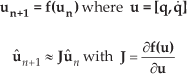
Determination of the equations of motion between collisions is straight forward and can be achieved Newton-Euler equation. Models have two independent degrees of freedom, the stance leg angle θ and the swing leg angle φ with respect to stance leg. Models are assumed M>>m and l/g=1. The equations of motion are generally given by:

$M(q)\stackrel{.}{q}+V(q,\stackrel{.}{q})+G(q)=0$

(1)

where q = [θ φ]^T and M is mass matrix. V is centrifugal and coriolis term and G is gravity term.

For the simplest walking model, as presented in [6],

$\begin{array}{c}M(q)=\left[\begin{array}{cc}1& 0\\ 1-\cos \varphi & -1\end{array}\right],\\ V(q,\stackrel{.}{q})+G(q)=\left[\begin{array}{c}\sin (\gamma -\theta )\\ \sin \varphi {\stackrel{.}{\theta }}^2-\sin (\gamma +\varphi -\theta )\end{array}\right]\end{array}$

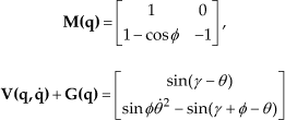
it has one free parameter γ (slope angle). Equations describe double inverted pendulum on a slope.

Modified models have more free parameters than the simplest walking model.

For curved feet model,

$\begin{array}{c}M(q)=\left[\begin{array}{cc}1-2r(1-r)(1-\cos \theta )& 0\\ 1-(1-r)\cos \varphi -r\cos (\theta -\varphi )& -1\end{array}\right],\\ V(q,\stackrel{.}{q})+G(q)=\left[\begin{array}{c}-(1-r)r\sin \theta {\stackrel{.}{\theta }}^2+r\sin \gamma +(1-r)\sin (\gamma -\theta )\\ (1-r)\sin \varphi {\stackrel{.}{\theta }}^2-\sin (\gamma +\varphi -\theta )\end{array}\right]\end{array}$

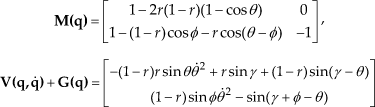
r (radius of foot) is another free parameter for curved feet model.

For flat feet model during swing phase 1 (rotating on heel) as shown in Fig. 3,

Figure 3.

Swing phase and collision of models.

$\begin{array}{c}M(q)=\left[\begin{array}{cc}{c}^2+1& 0\\ 1-\cos \varphi -c\sin \varphi & -1\end{array}\right],\\ V(q,\stackrel{.}{q})+G(q)=\left[\begin{array}{c}\sin (\gamma -\theta )+c\cos (\gamma -\theta )\\ (\sin \varphi -c\cos \varphi ){\stackrel{.}{\theta }}^2-\sin (\gamma +\varphi -\theta )\end{array}\right]\end{array}$

For flat feet model during swing phase 2 (rotating on toe),

$\begin{array}{c}M(q)=\left[\begin{array}{cc}{d}^2+1& 0\\ 1-\cos \varphi +d\sin \varphi & -1\end{array}\right],\\ V(q,\stackrel{.}{q})+G(q)=\left[\begin{array}{c}\sin (\gamma -\theta )-d\cos (\gamma -\theta )\\ (\sin \varphi +d\cos \varphi ){\stackrel{.}{\theta }}^2-\sin (\gamma +\varphi -\theta )\end{array}\right]\end{array}$

c (the distance from heel to ankle) and d (the distance from ankle to toe) are free parameters for flat feet model.

Equation of the motion during swing phase 2 is similar to that for the swing phase 1. Just the parameter c is changed to -d.

When foot shape parameters of modified models close to zero, equation of motion becomes the same as that of the simplest walking model.

2.3 Transition rule at collision

Models walk down under the influence of gravity, governed by the equations of motion, until the next leg hits the slope. It is assumed that the collision is fully inelastic impact. That means there are no slip and no bounce at contact point. Also, collision occurs instantaneously and the previous stance leg leaves the slope in the same instant and the new stance leg makes contact. It is assumed that there is an instantaneous impulse applied at the point of impact, which causes a discontinuous change in velocity.

Thus, angular momentum about the impact point will be conserved. From angular momentum conservation law, the transition rules are given by:

$H^{+}(q){\stackrel{.}{q}}^{+}=H^{-}(q){\stackrel{.}{q}}^{-}$

(2)

where q = [θ φ]^T and super scripts, “+” and “-”, means just after collision and just before collision.

Point feet model and curved feet model have just one collision, heel-strike, at every step as shown in Fig. 3. For flat feet model, there are two collisions at every step. At the end of the swing phase 1, toe-strike occurs. After that, it rotates on toe and heel-strike occurs at the end of swing phase 2.

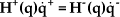
For the simplest walking model as presented in [6], the heel-strike occurs when the geometric collision condition

${\theta }^{+}=-{\theta }^{-}, {\varphi }^{+}=-2{\theta }^{-}$

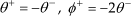
is satisfied. The matrix H is given by:

$H^{+}(q)=\left[\begin{array}{cc}1& 0\\ 1-\cos {\varphi }^{+}& -1\end{array}\right],H^{-}(q)=\left[\begin{array}{cc}\cos {\varphi }^{-}& 0\\ 0& 0\end{array}\right]$

For curved feet model, the geometric collision condition

${\theta }^{+}=-{\theta }^{-},{\varphi }^{+}=-2{\theta }^{-}$

is the same as that of the simplest walking model.

The matrix H is given by:

$\begin{array}{c}{H}^{+}(q)=\left[\begin{array}{cc}1-2r(1-r)(1-\cos {\theta }^{+})& 0\\ 1-(1-r)\cos {\varphi }^{+}-r\cos ({\theta }^{+}-{\varphi }^{+})& -1\end{array}\right],\\ H^{-}(q)=\left[\begin{array}{cc}\begin{array}{l}{r}^2+r(1-r)(\cos {\theta }^{-}+\cos ({\theta }^{-}-{\varphi }^{-}))\\ +{\left(1-r\right)}^2\cos {\varphi }^{-}\end{array}& 0\\ r-r\cos {\theta }^{-}& 0\end{array}\right]\end{array}$

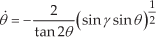
For flat feet model, toe-strike occurs when the geometric condition

${\theta }^{+}={\theta }^{-}=0,{\varphi }^{+}={\varphi }^{-}$

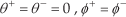
is met. The matrix H is given by:

$\begin{array}{c}{H}^{+}(q)=\left[\begin{array}{cc}1+d^2& 0\\ 1-\cos {\varphi }^{+}+d\sin {\varphi }^{+}& -1\end{array}\right],\\ H^{-}(q)=\left[\begin{array}{cc}1-cd& 0\\ 1-(\cos {\varphi }^{-}+c\sin {\varphi }^{-})& -1\end{array}\right]\end{array}$

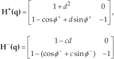
heel-strike occurs when the geometric condition

$\begin{array}{c}{\theta }^{+}=-{\varphi }^{-}+{\theta }^{-},{\varphi }^{+}=-{\varphi }^{-},\\ {\varphi }^{-}={\theta }^{-}-{\cos }^{-1}((k-c{(1+c^2-k^2)}^{\frac{1}{2}})∕(1+c^2))\end{array}$

where k=dsin(−θ⁻)+cos(−θ⁻) is met. The matrix H is given by:

$\begin{array}{c}{H}^{+}(q)=\left[\begin{array}{cc}1+c^2& 0\\ 1-\cos {\varphi }^{+}-c\sin {\varphi }^{+}& -1\end{array}\right],\\ H^{-}(q)=\left[\begin{array}{cc}(1-cd)\cos {\varphi }^{-}-(c+d)\sin {\varphi }^{-}& 0\\ 0& 0\end{array}\right]\end{array}$

Transition rules of modified models also become the same as those of the simplest walking model when foot shape parameters of modified models close to zero. It is noted that toe-strike does not occur for flat feet model in this case.

2.4 Proper initial condition

To get stable walking, one has to solve equation of motion and transition rule with proper initial conditions. Usually, arbitrary initial conditions lead to falling forward or backward. It is important to start with proper initial conditions which can lead to stable walking. Garcia et al. conceived proper initial conditions from the linearized equation of motion of the simplest walking model [6]. However, it is difficult to solve nonlinear differential equations of motion analytically if the model is complex like modified models.

In this work, we use falling boundary and energy balance line to get proper initial conditions. Those ideas are conceived and explained in appendix A.

3. Local stability analysis and bifurcation route to chaos

3.1 Local stability analysis

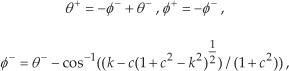
Every step can be considered as a function f(u). This function is a Poincaré map or is called stride function. The stride function f(u) can be obtained from equations of motion and transition rules explained in section 2.

$\begin{array}{c}{u}_{n+1}=f(u_n) \text{where} u=[q,\stackrel{.}{q}]\\ {\widehat{u}}_{n+1}\approx J{\widehat{u}}_n \text{with} J=\frac{\partial f(u)}{\partial u}\end{array}$

If u_n+1 = u_n, u_n is a fixed point on Poincaré map. Local stability is analyzed around fixed point on Poincaré map. Jacobian matrix J is calculated by perturbation method. û _n is a small perturbation. The eigenvalues of J quantify the stability of the cyclic motion of the walking models. If the eigenvalues of J are smaller than 1 in magnitude, the

small perturbation of the system will return to its limit cycle. It means the model is asymptotically stable.

If the eigenvalue of J are larger than 1 in magnitude, the cyclic motion is unstable. This stability analysis is valid only for small perturbation around fixed point. On the range of slope angles where the eigenvalue is smaller than 1 in magnitude, all the model walk stably with same step size and period. It is called period-one gait.

The largest eigenvalue of models increases with increasing the slope angle as shown in Fig. 4 and Fig. 5. Although slope angle increases, eigenvalue of leg angle is less than 1 in magnitude because of the collision condition. Meanwhile, eigenvalue of angular velocity become larger than 1 in magnitude at some slope angle. This characteristic is consistent with all models. It means models cannot handle perturbation about angular velocity as increasing slope angle.

Figure 4.

Eigenvalue of Jacobian of curved feet model.

Figure 5.

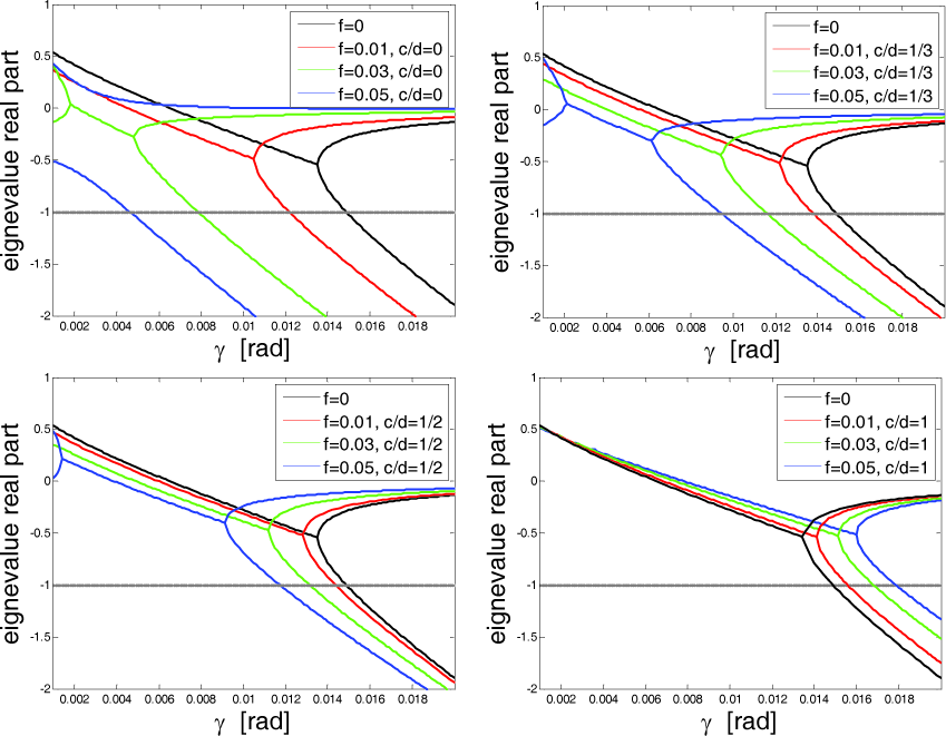
Eigenvalue of Jacobian of flat feet model.

From the result of Garcia et al, the simplest walking model has a stable period-one gait for slopes up to 0.0151[rad] [6]. For curved feet model, as the radius of foot increases, the eigenvalue becomes lager than 1 in magnitude on steeper slope compared to that of the simplest walking model. For example, when r=0.1, it has a stable period-one gait for slopes up to 0.0181[rad]. This implies that adding curved feet to a model can make walking more stable with increasing foot shape parameter. Similarly, when c/d=1 and f becomes larger, flat feet model has a stable period-one gait on steeper slope. It has a stable period-one gait for slopes up to 0.0180[rad] when f=0.05. Though similar result also can be found in [11], we consider the case of c/d<1 here. In contrast to c/d=1, as the foot length of the flat feet models increases, the eigenvalue becomes lager than 1 in magnitude on lower slope, if c/d<1. When c/d=1/3 and f=0.05, it has a stable period-one gait for slopes up to 0.0095[rad]. For the case with fixed foot length, the ratio (c/d) becomes larger the eigenvalue becomes lager than 1 on steeper slope. It means the model walks stably on steeper slopes as increasing distance from heel to ankle.

3.2 Bifurcation route to chaos

Period-one gait cycle exists on the range of slope angles where the eigenvalue is smaller than 1 in magnitude. Over this range, stable period-n gait cycle (n≥2) appears. When one of the eigenvalue passes through −1, bifurcation occurs. Then, stable period-two gait cycle appears. If u* is fixed point of function, a period-two gait cycle returns the same variable values after two steps: u* = f(f(u*)), and so on. After this chaotic motion, models fall down. There is no stable walking.

Though the range of period-one gait cycle can be known from the local stability analysis, the range of period-n gait cycle is not. The range of period-n gait cycle is confirmed by bifurcation diagram as shown in Fig. 6 and Fig. 7. Stable walking range of models is determined as shown in Table. 1. It is known that adding curved feet or flat feet with c/d=1 is advantageous to walk steep slope. In case of flat feet model with c/d<1, it cannot walk steep slope even if foot length increases.

Figure 6.

Bifurcation diagram of flat feet model.

Figure 7.

Bifurcation diagram of curved feet model.

Table 1.

Stable walking range of models.

Model	Foot shape parameter		Period-one gait [rad]	Period-n gait (n≥2) [rad]
Simplest walking model	r=0 or f=0		0<γ<0.0151	γ <0.0190
Curved feet model	r=0.05		0<γ<0.0165	γ <0.0210
	r=0.1		0<γ<0.0181	γ <0.0232
	r=0.15		0<γ<0.0200	γ <0.0257
Flat Feet model	c/d =0	f=0.01	0<γ<0.0123	γ <0.0165
		f=0.03	0<γ<0.0079	γ <0.0124
		f=0.05	0<γ<0.0047	γ <0.0092
	c/d =1/3	f=0.01	0<γ<0.0140	γ <0.0181
		f=0.03	0<γ<0.0117	γ <0.0163
		f=0.05	0<γ<0.0095	γ <0.0144
	c/d =1/2	f=0.01	0<γ<0.0145	γ <0.0187
		f=0.03	0<γ<0.0133	γ <0.0178
		f=0.05	0<γ<0.0119	γ <0.0169
	c/d =1	f=0.01	0<γ<0.0158	γ <0.0199
		f=0.03	0<γ<0.0169	γ <0.0215
		f=0.05	0<γ<0.0180	γ <0.0230

4. Global stability analysis

4.1 Cell-to-cell mapping

The eigenvalues of Jacobian quantifies the convergence time about small perturbations while global stability corresponds to the size of a perturbation. Global stability is determined by walking model's basin of attraction. If one can get stable gait cycle from proper initial conditions, there exist fixed point and a set of proper initial conditions around it. The set of proper initial conditions is called basin of attraction. The larger of basin of attraction gives more stable walking and can resist against to larger disturbances. We used cell-to-cell mapping method to investigate the basin of attraction, just like Schwarb and Wisse [7]. They applied the cell-to-cell mapping method to the simplest walking model and obtained a small, pointy boomerang-like basin of attraction.

Cell-to-cell mapping is applied as below [13]. The region of feasible initial conditions is subdivided into a large number(N) of small cells. Others are regarded as a very large cell called sink cell. All cells are numbered 1 to N+1. Then, center of each cell is applied to stride function f(u). Starting with cell numbered 1, mapping ends in a sink cell or in a repetitive cell including fixed point. When a fixed point is found, all cells in the mapping sequence are labeled as basin of attraction of the fixed point. This procedure is repeated with cell numbered 2, 3, and so on. If current sequence is encountered with already labeled cell from previous sequence, current sequence is merged with that of the already labeled cell. This procedure is repeated until N+1 cells are labeled.

4.2 Basin of attraction

Basin of attraction of models is obtained at fixed slope angle (γ=0.004[rad]). For curved feet model, basin of attraction is obtained with application of the cell-to-cell mapping with a discretization of about 200×200 points.

300×300 points are used for flat feet model. The results are shown in Fig. 8 and Fig. 9. Colored area is basin of attraction of each case. Solid line represents falling boundary and dashed line is energy balance line. These lines of models are expressed in appendix A. Falling boundary divides phase plane into two regions as shown in Fig. 10. Lower side of boundary is falling forward region and the other is falling backward region. Fixed point, marked with a pentagram is located on energy balance line. It is known that basin of attraction is located in falling forward region and is distributed near fixed point. Thus, it is possible to explain location of basin of attraction with these two lines in phase plane. Falling boundary of modified models moves right direction and energy balance line moves downward with varying foot shape parameters. Thus, basin of attraction moves in the right lower area in phase plane. It means that leg angle and angular velocity, proper initial conditions for stable walking, increase by adding two kinds of feet.

Figure 8.

Basin of attraction of curved feet models.

Figure 9.

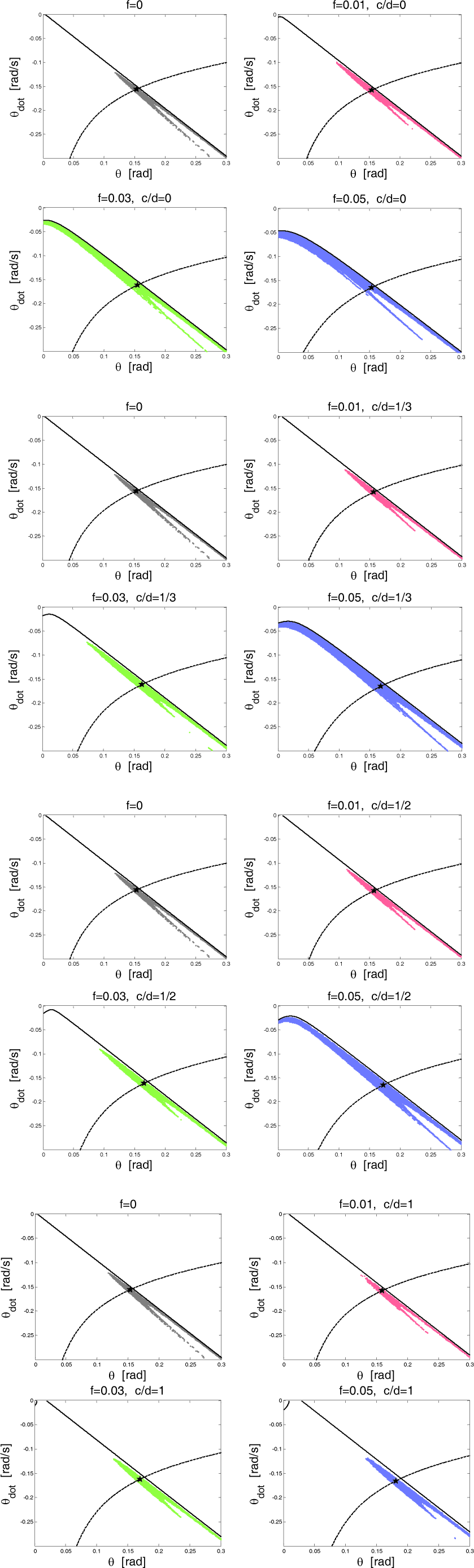
Basin of attraction of flat feet models.

Figure 10.

Basin of attraction of the simplest walking model and its falling boundary and energy balance line.

To compare the size of basin of attraction, area of basin of attraction of modified model is divided with that of the simplest walking model as shown in Table. 2. Basin of attraction of curved feet model is enlarged gradually with increasing its foot shape parameter. When r=0.15, the normalized area of basin of attraction is 1.88. It means this model is less sensitive to the initial condition and is easier to start stable walking than the simplest walking model by adding curved feet. Also, it is observed similar trend for flat feet model. The area of basin of attraction is enlarged with varying the foot length and ratio(c/d) except in the case of c/d=1 and f=0.01. When c/d=1/3 and f=0.05, the normalized area of basin of attraction become about five times larger than the simplest walking model's case. For f=0.01 and f=0.03, c/d becomes smaller but area of basin of attraction becomes larger. Although maximum area for f=0.05 is appeared at c/d=1/3 (not at c/d=0), All the cases show basin of attraction is enlarged in range of c/d<1 for the fixed foot length. It means decreasing distance from heel to ankle can be helpful to enlarge the basin of attraction. This is opposite to the result in section 3.

Table 2.

Area of basin of attraction of models.

Model	Foot shape parameter		Normalized area of basin of attraction
Curved feet model	r=0.05		1.30
	r=0.1		1.55
	r=0.15		1.88
Flat Feet model	c/d=0	f=0.01	1.43
		f=0.03	3.77
		f=0.05	4.41
	c/d=1/3	f=0.01	1.26
		f=0.03	2.28
		f=0.05	4.99
	c/d=1/2	f=0.01	1.23
		f=0.03	1.98
		f=0.05	4.46
	c/d=1	f=0.01	0.87
		f=0.03	1.53
		f=0.05	1.85

5. Conclusion

In this work, we analyzed the stability properties of modified feet models and compared the results to those of the simplest walking model whose stability properties are already well-known. From the results of local stability analysis and bifurcation diagram, stable walking range is obtained with respect to slope angle. Curved feet model walks stably on steeper slopes as increasing the radius of foot. Flat feet model can walk steeper slopes when c/d=1 while it can't walk on steeper slopes when c/d<1, even if its foot length increases. Thus, to make the model walks stably on steeper slopes, it can be helpful increasing distance from heel to ankle for fixed foot length. From the results of global stability analysis, curved feet model has lager basin of attraction with increasing the radius of foot. For flat feet model, the area of basin of attraction is enlarged with varying the foot length and ratio(c/d) except in the case of c/d=1 and f=0.01. All the cases for fixed foot length show basin of attraction enlarger in range of c/d<1 than c/d=1. It means decreasing distance from heel to ankle can be helpful to enlarge the basin of attraction.

These results are can be helpful when designing a biped robot and analyzing human gait.

6. Appendix A: Energy balance line and falling boundary

A.1 Energy balance line

For the simplest walking model,

$\stackrel{.}{\theta }=-\frac{2}{\tan 2\theta }{\left(\sin \gamma \sin \theta \right)}^{\frac{1}{2}}$

For curved feet model,

$\stackrel{.}{\theta }=-{\left(\frac{4\sin \gamma ((1-r)\sin \theta +r\theta ))}{({(1-r)}^2+r^2+2r(1-r)\cos \theta )(h_1{}^2-1)}\right)}^{\frac{1}{2}}$

where $h_1=\frac{{(1-r)}^2+2r(1-r)\cos \theta +r^2}{{(1-r)}^2\cos 2\theta +2r(1-r)\cos \theta +r^2}$ .

For flat feet model,

$\stackrel{.}{\theta }=-{\left[\frac{2(c^2+1)(d^2+1)(\mathrm{\Delta }P{E}_2-\mathrm{\Delta }P{E}_1)+2{(1-cd)}^2\mathrm{\Delta }P{E}_1}{(c^2+1)(d^2+1)((d^2+1)h_2{}^2-(c^2+1){(1-cd)}^2)}\right]}^{\frac{1}{2}}$

where

$\begin{array}{c}\mathrm{\Delta }P{E}_1=c\sin (\theta -\gamma )+\cos (\theta -\gamma )+c\sin \gamma -\cos \gamma ,\\ \begin{array}{c}\mathrm{\Delta }P{E}_2=c\sin (\theta -\gamma )+\cos (\theta -\gamma )+(c+d)\sin \gamma -\cos \gamma \\ -d\sin (\varphi -\theta +\gamma )-\cos (\varphi -\theta +\gamma )\end{array},\\ h_2=\frac{1+c^2}{(1-cd)\cos \varphi -(c+d)\sin \varphi },\\ \varphi =\theta +{\cos }^{-1}((k-d{(1+d^2-k^2)}^{\frac{1}{2}})∕(1+d^2)),\end{array}$

and k = csinθ + cosθ.

A2 Falling boundary

For the simplest walking model,

$\stackrel{.}{\theta }=\{\begin{array}{l}00\le \theta \le \gamma \\ -{\left[2(1-\cos (\theta -\gamma ))\right]}^{\frac{1}{2}}\gamma <\theta \le \pi ∕2\end{array}$

For curved feet model,

$\stackrel{.}{\theta }=\{\begin{array}{l}00\le \theta \le \gamma \\ -{\left[\frac{2(1-r)(1-\cos (\theta -\gamma ))+r\sin \gamma (\gamma -\theta )}{{(1-r)}^2+r^2+2r(1-r)\cos \theta }\right]}^{\frac{1}{2}}\gamma <\theta \le \pi ∕2\end{array}$

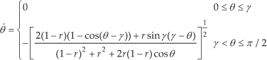
For flat feet model,

Case 1. tan⁻¹(d)≤γ

$\stackrel{.}{\theta }=\{\begin{array}{l}00\le \theta \le {\tan }^{-1}c+\gamma \\ -{\left(\frac{2\mathrm{\Delta }P{E}_1{}^{\text{'}}}{c^2+1}\right)}^{\frac{1}{2}}{\tan }^{-1}c+\gamma <\theta \le \pi ∕2\end{array}$

Case 2. ${\tan }^{-1}(d)>\gamma$

if $c^2+1-p^2<0$

$\stackrel{.}{\theta }=-{\left(\frac{2\mathrm{\Delta }P{E}_2{}^{\text{'}}}{(d^2+1)h_3{}^2}-\frac{2\left(\mathrm{\Delta }P{E}_1\right)}{c^2+1}\right)}^{\frac{1}{2}}0\le \theta \le \pi ∕2$

otherwise,

$\stackrel{.}{\theta }=\{\begin{array}{l}-{\left(\frac{2\mathrm{\Delta }P{E}_2{}^{\text{'}}}{(d^2+1)h_3{}^2}-\frac{2\left(\mathrm{\Delta }P{E}_1\right)}{c^2+1}\right)}^{\frac{1}{2}}0\le \theta \le {\cos }^{-1}q\\ 0{\cos }^{-1}q<\theta \le {\tan }^{-1}c+\gamma \\ -{\left(\frac{2\mathrm{\Delta }P{E}_1{}^{\text{'}}}{c^2+1}\right)}^{\frac{1}{2}}{\tan }^{-1}c+\gamma <\theta \le \pi ∕2\end{array}$

where

$\begin{array}{c}\mathrm{\Delta }P{E}_1=c\sin (\theta -\gamma )+\cos (\theta -\gamma )+c\sin \gamma -\cos \gamma ,\\ \mathrm{\Delta }P{E}_1{}^{\text{'}}=\sqrt{c^2+1}-c\sin (\theta -\gamma )-\cos (\theta -\gamma ),\\ \mathrm{\Delta }P{E}_2{}^{\text{'}}=\sqrt{d^2+1}-d\sin \gamma -\cos \gamma ,\\ q=\frac{p+c\sqrt{c^2+1-p^2}}{1+c^2},\\ p=\frac{(c^2+1)}{(d^2+1)h_3{}^2}\mathrm{\Delta }P{E}_2{}^{\text{'}}+\cos \gamma -c\sin \gamma \text{and} h_3=\frac{1-cd}{1+d^2}.\end{array}$