Sage Journals: Discover world-class research

Abstract

To achieve high walking stability for a passive dynamic walking robot is not easy. In this article, we aim to investigate whether the walking performance for a passive dynamic walking robot can be improved by just simply changing the swing ankle angle before impact. To validate this idea, a passive bipedal walking model with two straight legs, two flat feet, a hip joint, and two ankle joints was built in this study. The walking dynamics that contains double stance phase was derived. By numerical simulation of the walking in MATLAB, we found that the walking performance can be adjusted effectively by only simply changing the swing ankle angle before impact. A bigger swing ankle angle in a reasonable range will lead to a higher walking stability and a lower initial walking speed of the next step. A bigger swing ankle angle before impact leads to a bigger amount of energy lost during impact for the quasi-passive dynamic walking robot which will influence the walking stability of the next step.

Keywords

Walking dynamics passive dynamic walking robot biped robot numerical simulation walking stability step length step duration

Introduction

Bipedal walking robot research is a popular area in robotics research due to its high resemblance to humans. During the past decades, several bipedal robots have been built. The famous bipedal walkers, ASIMO¹ and NAO,² exhibit versatile gaits when walking and walk with a high stability and robustness. However, such robot features high energy consumption³ and unnatural gait during walking because of their zero moment point (ZMP)⁴-based static walking control strategy. The concept of “passive dynamic walking”^5,6 provides a possible way to develop more human-like robot. However, the fully passive dynamic walking robot is very sensitive to its initial condition and can only walk successfully within a range of slopes. In order to achieve level ground walking, several quasi-passive dynamic walking robot^7–9 have been built, in which some joints are driven by motors or pneumatic muscles.

The passive dynamic walker is more sensitive to its mechanical construction and mechanical parameters than the active robot because not all the joints are controlled. To improve this situation, several studies have been reported to explore more reasonable mechanical construction and optimized mechanical parameters to obtain better walking stability and efficiency. It is found that passive robot with flat feet with springs can obtain better walking stability than that with curved feet or with the feet without ankle compliance.^10,11 It is also found that adding an upper body to the passive robot can enhance the walking stability to the robot.¹² Different types of passive models^13–15 were optimized to obtain a better walking performance based on the local stability analysis or global stability analysis with cell mapping method.¹⁶ The optimal mechanical structure of the passive robot in Collins et al.¹⁷ is obtained based on several times “trail, error and correction” process in experiments.

In addition, because only few joints are actuated, the common effective control idea, such as the “hybrid zero dynamics”¹⁸ that is well used on the under-actuated dynamic biped robot such as RABBIT,¹⁹ is hard to apply to the passive dynamic robot. So, usually the control for passive dynamic walkers is applied to prevent falling forward or backward in a catch-up way to keep dynamic equilibrium during walking but not to define the exact joint trajectories. It is found that the limit cycle walker will never fall forward if the swing leg swings forward fast enough and will not fall backward if the stance leg angle is not too big,²⁰ which has been proved effective to guide control method design in some other works.^21,22 MW Spong et al.²³ used virtual gravity principle to control a compass gait robot walking on level ground in simulation. The energy consumption is very low, but it is hard to apply it on a real robot. In Schuitema et al.,⁹ a reinforcement learning-based controller is applied to a five-link passive robot which can deal with 1 cm step-down during walking. Hobbelen and Wisse²¹ applied local ankle feedback control and ankle push-off to control a limit cycle walker which can walk over a 3 cm step-down successfully. It is also found that the posture of the robot has a big effect on the energy lost at impact,²⁴ which could affect the walking performance definitely. The swing leg retraction method to improve the waking stability for a passive dynamic walker proposed in Hobbelen and Wisse²⁵ is based on this idea. So, this study aims to investigate whether we can improve the walking performance for a passive dynamic walking robot by just simply changing the swing ankle angle so that to adjust the robot posture before impact.

In this study, a fully passive dynamic walking model that consisted of two straight legs, two flat feet, two ankle joints, and a hip joint was built. A detailed walking dynamics that contains double stance phase was derived based on the virtual power principle.^14,26 Numerical simulations were performed in MATLAB. The influence of the swing ankle angle on walking stability, step length and step duration was analyzed. The effect of different values of the swing ankle angle on walking stability of the quasi-passive dynamic walker was also analyzed by observing the amount of lost energy during impact.

The article is organized as follows. In section “Walking dynamics,” we derive the walking dynamics. In section “Numerical simulation and results,” we introduce the numerical simulation process and the simulation results. In section “Effect of swing ankle angle’s value on walking performance,” detailed analysis based on the simulation results is discussed. We conclude in section “Conclusion.”

Walking dynamics

Walking phases

To study the influence of the swing ankle angle on walking performance, a passive walking model that consisted of two straight legs, two flat feet, two ankle joints, and a hip joint was built, as shown in Figure 1, where $θ_{1}, θ_{2}, θ_{3}, and θ_{4}$ denote the trailing leg, leading leg, trailing foot, and leading foot angle, respectively. C₁, C₂, C_f₁, and C_f₂ denote the position of the center of mass (COM) for the trailing leg, leading leg, trailing foot, and leading foot, respectively. K_h and k_a denote the joint spring stiffness at the hip and ankle joints, respectively.

Figure 1.

Passive dynamic walking model.

We only focus on the influence of the swing ankle just before impact, so straight leg without knee joints is enough for our analysis.

Double stance phase (i.e. both feet contact with the ground at the same time) exists in human and animal walking.²⁷ So there is double stance phase during walking in this study. One typical walking phase contains “first impact phase,”“first double stance phase,”“second impact phase,”“second double stance phase,” and “swing phase,” as depicted in Figure 2. The red cycles in the feet represent the constraints exerted by the ground contact forces in Figure 2.

Figure 2.

Walking phases in one walking step.

Phase a: First impact phase

The swing foot’s heel impacts with the ground and the old swing leg becomes the new stance (i.e. leading) leg (dotted line in Figure 2), and the old stance leg becomes the new trailing leg (solid line in Figure 2). Typically, the instant just after impact is chosen as the initial condition of the walking. However in this article, to decrease the number of independent initial state variables, the instant just before heel impact is chosen as the start of the walking.

Phase b: First double stance phase

The trailing leg’s toe and the leading leg’s heel keep contact with the ground at the same time. Whether the trailing leg’s heel keeps contact with the ground depends on where the ground reaction force under the trailing leg happens. In this article, we can find that the trailing leg’s heel loses contact immediately after the first impact, which will be discussed in detail in the following section. So the robot rotates forward around the trailing foot’s toe and the leading foot’s heel.

Phase c: Second impact phase

When the leading foot rotates to a proper angle, the second impact happens. The leading toe impacts with the ground and then the leading foot keeps full contact with the ground.

Phase d: Second double stance phase

The trailing foot’s toe and the whole leading foot keep contact with the ground at the same time. The robot rotates forward around the trailing foot’s toe and the leading foot’s ankle joint.

Phase e: Swing phase

When the trailing foot’s toe loses contact with the ground, the walking comes to the swing phase. The leading leg rotates forward around the ankle joint and the swing leg rotates forward around the hip joint. The leading foot is kept at a constant angle with respect to the leading leg in this phase by the constraint in equation (20). This phase ends before the instant that the swing heel impacts with the ground again. Then, the robot will repeat these phases to keep walking.

Walking dynamics

The parameters and their default values are listed in Table 1. The values are determined based on the analogy to human body parameters. The values for k_h and k_a are determined by several times tuning in simulation to find the fixed point.²⁸ To make the simulation results more universal, all the parameters are transferred to their dimensionless form. The parameters related to length is obtained by dividing l, the parameters related to mass is obtained by dividing M which denotes the total mass of the robot, the parameters related to moment of inertial is obtained by dividing Ml², the time is obtained by dividing (l/g)^1/2 and the spring stiffness is obtained by dividing Mg/l.

Table 1.

Mechanical parameters and their default values.

Parameter	Description	Dimensionless value
l	Leg length	1
l_f	Foot length	0.25
l_f ₁	Frontal foot length (from toe to ankle)	0.2
l_f ₂	Hinder-foot length (from ankle to heel)	0.05
b_l	Leg COM (from COM position to hip)	0.5
b_f	Foot COM (from COM position to heel)	0.1
m_h	Hip mass	0.4
m_f	Foot mass	0.05
m_l	Leg mass	0.25
J_h	Hip moment of inertia	0
J_f	Foot moment of inertia	0.0016
J_l	Leg moment of inertia	0.015
β	Slope angle	3 (°)
K_h	Hip joint spring stiffness	0.4
k_a	Ankle joint spring stiffness	0.6

COM: center of mass.

Usually, we use the Poincare mapping method²⁸ to describe the periodic walking for a passive robot. We can choose a Poincare section through which the walking trajectory passes periodically at any instant of the Poincare mapping process, and the state on this section is chosen as the initial condition for the walking. If the robot can converge to one fixed initial condition after several steps, we deem that the walking is locally stable, and the converged initial condition is the so-called fixed point.²⁸

Usually, the instant just after foot–ground impact is chosen as the Poincare section. However, in this study, the instant just before foot–ground impact is chosen as the Poincare section (i.e. initial condition). If we choose the instant just before impact as the initial condition, the number of initial independent state variables can be reduced to three which are $θ_{1}, {\overset{\cdot}{θ}}_{1}, and {\overset{\cdot}{θ}}_{2}$ , and all other state variables can be described by the three initial independent state variables, as shown in equations (1) and (2). Fewer initial independent state variables enhance the chance of obtaining fixed point greatly. As mentioned above, the trailing foot is kept at a constant angle with respect to the trailing leg before impact, which means that ${\overset{\cdot}{θ}}_{3}^{-} = {\overset{\cdot}{θ}}_{1}^{-}$ . Like human-beings, we assume that the stance foot keeps full contact with the ground before the swing heel touches the ground as in equation (1). In equation (2), $θ_{w}$ is defined as the swing ankle angle that denotes the angle between the swing leg and the foot and the superscript “−” denotes the instant just before impact. In this article, the y-axis is set as the reference axis for $θ_{1}$ and x-axis is that for $θ_{3}$ , as shown in Figure 1. So the value of $θ_{w}$ is 0 when the actual physical angle between the swing leg and the foot is $π / 2$ . By changing the value of $θ_{w}^{-}$ , we can obtain different angle values for $θ_{3}^{-}$ as in equation (2). The value of $θ_{2}^{-}$ is obtained by the physical constraint of the robot just before impact as in equation (2)

{\begin{matrix} {\overset{\cdot}{θ}}_{3}^{-} = {\overset{\cdot}{θ}}_{1}^{-} \\ {\overset{\cdot}{θ}}_{4}^{-} = θ_{4}^{-} = 0 \end{matrix}

(1)

{\begin{matrix} θ_{3}^{-} = θ_{1}^{-} + θ_{w}^{-} \cdot \frac{π}{180} \\ θ_{2}^{-} = - \arccos (\frac{l_{f 1} \cdot \sin θ_{3}^{-} + l \cdot \cos θ_{1}^{-}}{l}) \end{matrix}

(2)

First impact phase

We assume that the foot–ground impact is instantaneous and fully inelastic, and the angles of each part cannot change suddenly at the instant just after impact. According to the angular momentum theorem, the angular momentum of the entire robot is conserved around the leading heel F2; the angular momentum of the leading leg, trailing leg, trailing foot, and hip is conserved around the leading ankle A1; the angular momentum of the trailing leg and trailing foot is conserved around the hip joint H; and the angular momentum of the trailing foot is conserved around the trailing leg ankle A2, as in equation (3)

{\begin{matrix} {\overset{\cdot}{x}}_{htt}^{+} = {\overset{\cdot}{x}}_{hlh}^{+} \\ {\overset{\cdot}{y}}_{htt}^{+} = {\overset{\cdot}{y}}_{hlh}^{+} \\ {\vec{L}}_{F 2}^{+} = {\vec{L}}_{F 2}^{-} + (x_{F 3} - r^{*} - x_{F 2}) \cdot I_{y}^{*} - (y_{F 3} - y_{F 2}) \cdot I_{x}^{*} \\ {\vec{L}}_{A 1}^{+} = {\vec{L}}_{A 1}^{-} + (x_{F 3} - r^{*} - x_{A 1}) \cdot I_{y}^{*} - (y_{F 3} - y_{A 1}) \cdot I_{x}^{*} \\ {\vec{L}}_{H}^{+} = {\vec{L}}_{H}^{-} + (x_{F 3} - r^{*} - x_{H}) \cdot I_{y}^{*} - (y_{F 3} - y_{H}) \cdot I_{x}^{*} \\ {\vec{L}}_{A 2}^{+} = {\vec{L}}_{A 2}^{-} + (x_{F 3} - r^{*} - x_{A 2}) \cdot I_{y}^{*} - (y_{F 3} - y_{A 2}) \cdot I_{x}^{*} \end{matrix}

(3)

In equation (3), ${\vec{L}}^{+}$ denotes the angular moment about a point just after impact and ${\vec{L}}^{-}$ denotes that just before impact, respectively. The left side of the first two equations is calculated based on the trailing leg’s toe–ground contact position, and the right side is calculated based on the leading leg’s heel–ground contact position, respectively. These two equations can guarantee the constraint that the trailing leg’s toe and the leading leg’s heel must keep contact with the ground without sliding and lifting during impact.

During impact, there are impulses both under the leading and trailing foot as the trailing leg will not lift up immediately. $I_{x}^{*}$ and $I_{y}^{*}$ denote the component of impulse along x-axis and y-axis under trailing foot, respectively in equation (3). Because the position where the impulse generates is unknown, a new parameter $r^{*}$ that denotes the distance from the trailing foot’s toe to the position that the impulse generates is introduced here. To solve $r^{*}$ , we assume that the trailing foot’s heel loses contact with the ground immediately after impact (i.e. the impulse generates at the toe point) first, and so $r^{*} = 0$ . There are six unknown parameters that are ${\overset{\cdot}{θ}}_{1}^{+}, {\overset{\cdot}{θ}}_{2}^{+}, {\overset{\cdot}{θ}}_{3}^{+}, {\overset{\cdot}{θ}}_{4}^{+}, I_{x}^{*}, and I_{y}^{*}$ , respectively, and can be solved by the six equations in equation (3). After we solve this equation, we examine the value of $I_{y}^{*}$ . If the value of $I_{y}^{*}$ is greater than 0, the trailing toe keeps contact with the ground indeed and thus we deem that the assumption about the value of $r^{*}$ is reasonable. If $I_{y}^{*} \leq 0$ , we deem that $r^{*} \neq 0$ , and thus the trailing foot keeps full contact with the ground during impact (i.e. ${\overset{\cdot}{θ}}_{4}^{+} = 0$ ). We can also solve all the unknown parameters in equation (3) with the additional function ${\overset{\cdot}{θ}}_{4}^{+} = 0$ .

First double stance phase

During this phase, the degree of freedom (DOF) of the system is 2, but the number of the generalized coordinates is 4. So the system is a holonomic system that contains redundant coordinates, and thus the Euler–Lagrange equation²⁹ cannot be applied here. The virtual power principle^14,26 is suitable in this phase, which can handle holonomic system that contains redundant coordinates or non-holonomic system.

The walking dynamics can be described by the rectangular coordinates x or the generalized coordinates q as follows

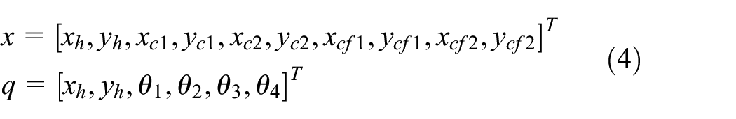
\begin{matrix} x = [x_{h}, y_{h}, x_{c 1}, y_{c 1}, x_{c 2}, y_{c 2}, x_{cf 1}, y_{cf 1}, x_{cf 2}, y_{cf 2}]^{T} \\ q = [x_{h}, y_{h}, θ_{1}, θ_{2}, θ_{3}, θ_{4}]^{T} \end{matrix}

(4)

In equation (4), the parameters in x denote the position of the COM of the hip, trailing leg, leading leg, trailing foot, and leading foot along x-axis and y-axis, respectively. For q, please see Figure 1. We add two extra redundant generalized coordinate x_h and y_h to the system, which will be discussed below.

The rectangular coordinates can be converted to the generalized coordinates as follows

x = x (q)

(5)

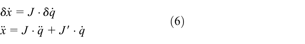
Convert equation (5) into its variation form and second differential form as well, and we can get equation (6)

\begin{matrix} δ \overset{\cdot}{x} = J \cdot δ \overset{\cdot}{q} \\ \overset{\cdot\cdot}{x} = J \cdot \overset{\cdot\cdot}{q} + J' \cdot \overset{\cdot}{q} \end{matrix}

(6)

where $J = \partial x / \partial q$ , $J' = \partial (J \overset{\cdot}{q}) / \partial q$ .

The virtual power approach follows the following form¹⁴ as follows

δ {\overset{\cdot}{x}}^{T} [f - M \overset{\cdot\cdot}{x}] = 0

(7)

Equation (7) means that the sum of the virtual power of the active forces and the inertial forces is zero at any instant for an ideal mass points system, so we convert it to the following form as

Δ P + Δ P^{*} = 0

(8)

Equation (8) is a general form for the virtual power principle, where $Δ P$ denotes the active force’s virtual power and $Δ P^{*}$ denotes the inertial force’s virtual power, respectively. The detailed forms of them are as follows

{\begin{matrix} Δ P = \sum_{i} f_{i} \cdot δ {\overset{\cdot}{x}}_{i} + \sum_{i} τ_{i} \cdot δ {\overset{\cdot}{q}}_{i} \\ Δ P^{*} = - \sum_{i} m_{i} {\overset{\cdot\cdot}{x}}_{i} \cdot δ {\overset{\cdot}{x}}_{i} - \sum_{i} I_{i} {\overset{\cdot\cdot}{q}}_{i} \cdot δ {\overset{\cdot}{q}}_{i} \end{matrix}

(9)

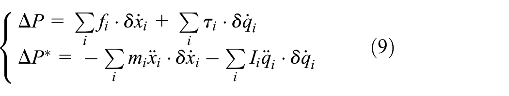
In equation (9), x_i and q_i denote each element in equation (4), respectively. Based on equation (6), we can convert equation (9) to its matrix form in generalized coordinates as follows

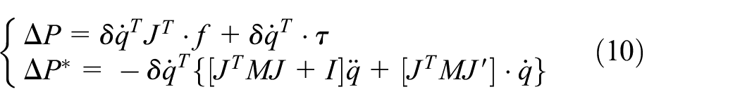
{\begin{matrix} Δ P = δ {\overset{\cdot}{q}}^{T} J^{T} \cdot f + δ {\overset{\cdot}{q}}^{T} \cdot τ \\ Δ P^{*} = - δ {\overset{\cdot}{q}}^{T} {[J^{T} MJ + I] \overset{\cdot\cdot}{q} + [J^{T} MJ'] \cdot \overset{\cdot}{q}} \end{matrix}

(10)

In equation (10), M denotes the mass matrix for each mass point (i.e. each COM of the robot), I denotes the moment of inertia matrix for each part of the robot, f denotes the force matrix which can be induced by gravity or other external forces, and $τ$ denotes the torque matrix to each generalized coordinate which can be induced by passive springs or active driving sources. In this article, all the torques exerted to each joints are induced by passive springs. The details of them are listed as follows

\begin{matrix} M = Diag (m_{h}, m_{h}, m_{l}, m_{l}, m_{l}, m_{l}, m_{f}, m_{f}, m_{f}, m_{f}) \\ I = Diag (J_{h}, J_{h}, J_{l}, J_{l}, J_{f}, J_{f}) \\ f = Mg [\sin (β), - \cos (β), \sin (β), - \cos (β), \\ \sin (β), - \cos (β), \sin (β), - \cos (β), \sin (β), - \cos (β)]^{T} \\ τ = [τ_{hx}, τ_{hy}, τ_{sw}, τ_{st}, τ_{f 1}, τ_{f 2}]^{T} \end{matrix}

(11)

The descriptions and values for all elements in equation (11) are listed in Table 1. Based on equation (10), we can transfer equation (8) to the following form

δ {\overset{\cdot}{q}}^{T} {J^{T} [f - MJ' \cdot \overset{\cdot}{q}] + τ - [J^{T} MJ + I] \overset{\cdot\cdot}{q}} = 0

(12)

Because the generalized coordinates are not all independent variables (i.e. the number of generalized coordinates is bigger than that of the DOF), we introduce $λ$ multiplier and the relative constraint function into the system, based on the Lagrange equation of first kind.^15,26

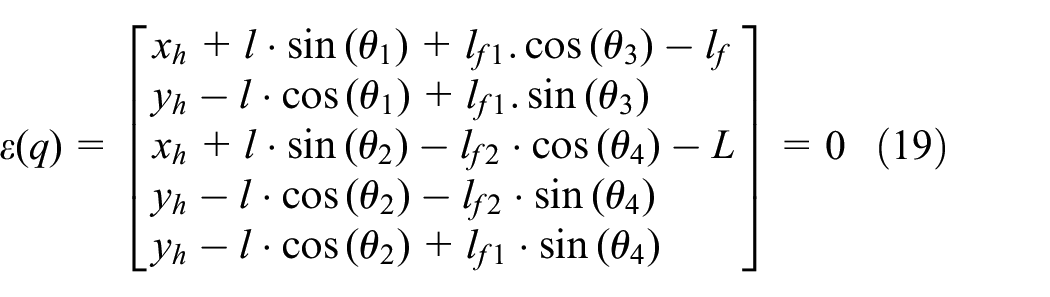
The instant when the trailing toe loses contact with the ground depends on the ground reaction force exerted on the toe and the direction of the acceleration of the toe–ground contact point.³⁰ So in order to solve the ground reaction force, at least two extra generalized coordinates $x^{h}$ and $y^{h}$ should be added to the system.

During this phase, the introduced constraint function mentioned above can be described as follows

ε (q) = [\begin{matrix} x_{h} + l \cdot \sin (θ_{1}) + l_{f 1} . \cos (θ_{3}) - l_{f} \\ y_{h} - l \cdot \cos (θ_{1}) + l_{f 1} . \sin (θ_{3}) \\ x_{h} + l \cdot \sin (θ_{2}) - l_{f 2} \cdot \cos (θ_{4}) - L \\ y_{h} - l \cdot \cos (θ_{2}) - l_{f 2} \cdot \sin (θ_{4}) \end{matrix}] = 0

(13)

In equation (13), L denotes the step length and can be handled as a constant value here. The first two constraint functions guarantee that the trailing leg’s toe must keep contact with the ground (i.e. the first two functions are the calculated position of the trailing toe along x-axis and y-axis, respectively). The second two constraint functions guarantee that the leading leg’s heel must keep contact with the ground (i.e. the second two functions are the calculated position of the leading heel along x-axis and y-axis, respectively). Transfer equation (13) into its variation form and multiply by the $λ$ multiplier as follows

δ {\overset{\cdot}{q}}^{T} \cdot T^{T} λ = 0

(14)

In equation (14), $T = \partial ε (q) / \partial q$ and $λ$ is the multiplier that denotes the constraint force induced by each constraint functions in equation (13).^15,26 In this phase, the first two elements of $λ$ denote the ground contact force under trailing toe along x-axis and y-axis, respectively, and the last two elements of $λ$ denote the ground contact force under leading heel along x-axis and y-axis, respectively.

On rearranging equations (12) and (14), we can get

[J^{T} MJ + I] \overset{\cdot\cdot}{q} = J^{T} [f - MJ' \cdot \overset{\cdot}{q}] + τ + T^{T} λ

(15)

Equation (13) can be converted into its second differential form

T \overset{\cdot\cdot}{q} + (\partial \frac{T \overset{\cdot}{q}}{\partial q}) \cdot \overset{\cdot}{q} = 0

(16)

On rearranging equations (15) and (16), we can obtain the walking dynamics in this phase as follows

[\begin{matrix} J^{T} MJ + I & - T^{T} \\ T & 0 \end{matrix}] [\begin{matrix} \overset{\cdot\cdot}{q} \\ λ \end{matrix}] = [\begin{matrix} J^{T} [f - MJ' \cdot \overset{\cdot}{q}] + τ \\ - (\partial (T \overset{\cdot}{q}) / \partial q) \cdot \overset{\cdot}{q} \end{matrix}]

(17)

Second impact phase

When the value of the leading toe along y-axis is equal to 0, the walking comes to the second impact phase. The assumption for this phase is the same as it is in the first impact phase. The angular momentum of the entire robot is conserved around the tailing toe F3; the angular momentum of the leading leg, leading foot, trailing leg, and hip is conserved around the trailing ankle joint A2; the angular momentum of the leading leg and leading foot is conserved around the hip joint H; the angular momentum of the leading foot is conserved around the leading leg ankle joint A1, as in equation (18)

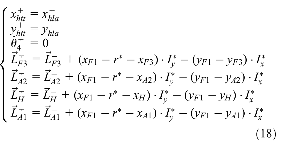
{\begin{cases} x_{h t t}^{+} = x_{h l a}^{+} \\ y_{h t t}^{+} = y_{h l a}^{+} \\ {\dot{θ}}_{4}^{+} = 0 \\ {\vec{L}}_{F 3}^{+} = {\vec{L}}_{F 3}^{-} + (x_{F 1} - r^{*} - x_{F 3}) \cdot I_{y}^{*} - (y_{F 1} - y_{F 3}) \cdot I_{x}^{*} \\ {\vec{L}}_{A 2}^{+} = {\vec{L}}_{A 2}^{-} + (x_{F 1} - r^{*} - x_{A 2}) \cdot I_{y}^{*} - (y_{F 1} - y_{A 2}) \cdot I_{x}^{*} \\ {\vec{L}}_{H}^{+} = {\vec{L}}_{H}^{-} + (x_{F 1} - r^{*} - x_{H}) \cdot I_{y}^{*} - (y_{F 1} - y_{H}) \cdot I_{x}^{*} \\ {\vec{L}}_{A 1}^{+} = {\vec{L}}_{A 1}^{-} + (x_{F 1} - r^{*} - x_{A 1}) \cdot I_{y}^{*} - (y_{F 1} - y_{A 1}) \cdot I_{x}^{*} \end{cases}

(18)

In equation (18), the first two equations guarantee the trailing toe and leading ankle keep contact with the ground in this phase as mentioned in the first impact phase. r* denotes the distance from the leading toe to the position where the impulse happens. We assume that the leading foot keeps full contact with the ground as mentioned above, which means that ${\overset{\cdot}{θ}}_{4}^{+} = 0$ . There are seven unknown parameters ${\overset{\cdot}{θ}}_{1}^{+}, {\overset{\cdot}{θ}}_{2}^{+}, {\overset{\cdot}{θ}}_{3}^{+}, {\overset{\cdot}{θ}}_{4}^{+}, I_{x}^{*}, I_{y}^{*}, and r^{*}$ , which can be solved by equation (18) directly.

Second double stance phase

The walking dynamics for this phase shares the same form as in the first double stance phase, as shown in equation (17). However, the constraint function for this phase is different from that in the first double stance phase. During this phase, the trailing toe still keeps contact with the ground, and the leading foot keeps full contact with the ground. So the constraint function in this phase is as follows

ε (q) = [\begin{matrix} x_{h} + l \cdot \sin (θ_{1}) + l_{f 1} . \cos (θ_{3}) - l_{f} \\ y_{h} - l \cdot \cos (θ_{1}) + l_{f 1} . \sin (θ_{3}) \\ x_{h} + l \cdot \sin (θ_{2}) - l_{f 2} \cdot \cos (θ_{4}) - L \\ y_{h} - l \cdot \cos (θ_{2}) - l_{f 2} \cdot \sin (θ_{4}) \\ y_{h} - l \cdot \cos (θ_{2}) + l_{f 1} \cdot \sin (θ_{4}) \end{matrix}] = 0

(19)

The first two constraint functions guarantee that the trailing leg’s toe must keep contact with the ground. The second two constraint functions guarantee that the leading leg’s heel must keep contact with the ground. The last function guarantees that the leading leg’s toe must keep contact with the ground (i.e. the last function is the calculated position of the leading toe along y-axis). The leading toe shares the same constraint function with the leading heel along x-axis as they are part of the same rigid leading foot so that three constraint functions are enough for the leading foot.

When the value of $λ$ multiplier under the second constraint function equals to 0, the walking robot comes to the swing phase. In other words, when the ground contact force under the trailing toe reduces to 0, the trailing foot loses contact with ground.

Swing phase

The walking dynamics for this phase shares the same form as in the first double stance phase, as shown in equation (17). However, the constraint function for this phase is different from that in the first double stance phase. During this phase, the leading foot keeps full contact with the ground. So the constraint function in this phase is as follows

ε (q) = [\begin{matrix} x_{h} + l \cdot \sin (θ_{2}) - l_{f 2} \cdot \cos (θ_{4}) - L \\ y_{h} - l \cdot \cos (θ_{2}) - l_{f 2} \cdot \sin (θ_{4}) \\ y_{h} - l \cdot \cos (θ_{2}) + l_{f 1} \cdot \sin (θ_{4}) \\ θ_{3} - θ_{1} - θ_{w} \cdot π / 180 \end{matrix}] = 0

(20)

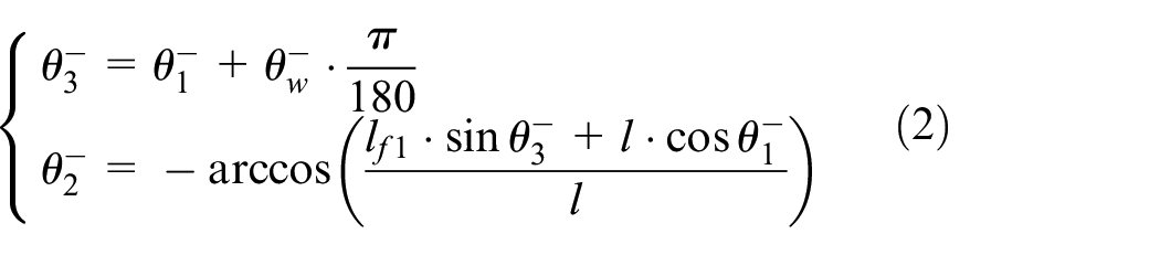
In equation (20), the last constraint function controls the angle between the swing leg and swing foot as mentioned in equation (1). When $θ_{w} = 0$ , this constraint function means that the swing foot keeps the same angle with the swing leg all over the swing phase. When the value of the trailing heel along y-axis is equal to 0, the walking comes to the first impact phase again and repeat the walking periodically.

Numerical simulation and results

Numerical simulation process

We perform the numerical simulation process in MATLAB based on the derived walking dynamics in section “Walking dynamics.” We can test whether the derived walking dynamics is correct by the simulation process and make further analysis based on the simulation results. To find out the fixed point, the Poincare mapping²⁸ function should be built first. The Poincare mapping function can be described in the following form as

x_{n + 1} = P (x_{n})

(21)

In equation (21), P is the Poincare function which describes the mapping from (nth) system initial state to the ((n + 1)th) system initial state. After several times of mapping, if the system state can converge to itself, we can say that the fixed point²⁸ is obtained, as in equation (22)

x^{*} = P (x^{*})

(22)

In other words, the Poincare mapping method can describe the walking process for one step. The input of this function is the initial condition for this step, and the output of this function is the ending of this step. The ending of this step can be used as the initial condition for the next step which forms a loop for the walking. The details of Poincare mapping function are described in Figure 3.

Figure 3.

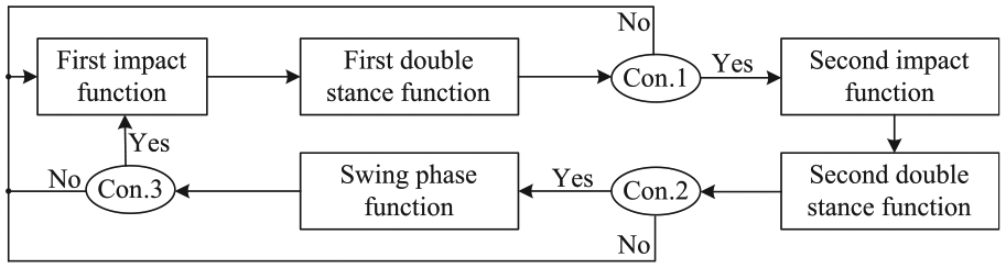
Details of Poincare mapping function.

As shown in Figure 3, we first use the “first impact function” as in equation (3). The result of this function is used as the initial condition for the “first double stance function” as in equation (17). This function is solved by the ODE45 algorithm in MATLAB. If the result of this function satisfies the condition 1, the robot comes to the second impact phase. If not, we return to the start of the walking and give another initial condition for the walking and perform the same loop. Condition 1 can be described as follows

y F_{1} = l_{f} \cdot \sin (θ_{4}) = 0

(23)

This function means that when the position of the leading toe along y-axis is equal to 0, the robot comes to the second impact phase. After this phase, the robot comes to the second double stance phase. The function in the second double stance phase is solved by the ODE45 algorithm in MATLAB as well. If the result of this function satisfies the condition 2, the robot comes to the swing phase. If not, we return to the start of the walking and give another initial condition for the walking and perform the same loop. Condition 2 can be described as follows

λ_{F 3} = 0

(24)

This function means that when the ground reaction force under the trailing leg’s toe is equal to 0, the robot comes to the swing phase. It can be solved by equation (17). The function in the swing phase is solved by the ODE45 algorithm in MATLAB as well. If the result of this function satisfies the condition 3, the robot comes to the first impact phase again. By now, one loop for the Poincare mapping function is ended. If not, we return to the start of the walking and give another initial condition for the walking and perform the same loop. Condition 3 can be described as follows

{\begin{matrix} θ_{2} < θ_{1} \\ vy A_{1} = - l_{f 1} \cdot \cos (θ_{4}) \cdot {\overset{\cdot}{θ}}_{4} - l \cdot \sin (θ_{2}) \cdot {\overset{\cdot}{θ}}_{2} + l \cdot \sin (θ_{1}) \cdot {\overset{\cdot}{θ}}_{1} < 0 \\ y F_{2} = - l_{f 1} \cdot \sin (θ_{4}) + l \cdot \cos (θ_{2}) - l \cdot \cos (θ_{1}) - l_{f 2} \cdot \sin (θ_{3}) = 0 \end{matrix}

(25)

The first equation guarantees that the swing leg must be at the front of the stance leg before impact. The second equation guarantees that the leading toe is in the state of falling-down, but not lifting-up. Taking the leading ankle to calculate the velocity gives a more precise prediction about whether the swing leg is swinging upward or downward than that of the leading heel. The last equation guarantees that the leading heel is going to impact with the ground immediately.

We use the Newton–Raphson iteration algorithm¹⁴ to obtain the fixed point based on the Poincare mapping function described above. After the fixed point has been obtained, we use it as the initial condition for the walking and perform the simulations based on the Poincare mapping function.

Simulation results

First, we set $θ_{w} = 0$ in equation (1) to perform the simulation process and find out the fixed point. After trying several times, we obtained the fixed point at x = [0.354381; −0.775042; −0.528854]. We took this as the initial condition of the walking and performed five steps simulation. As mentioned above, by taking the instant just before first impact as the start of the walking, the number of the independent initial state variables can be reduced to three, so there are only three elements for the fixed point. The walking gait analysis based on the simulation results is shown in Figure 4. Figure 4 shows the values of the legs and feet angle for two steps.

Figure 4.

(a) Swing and stance leg angle values and (b) Swing and stance feet angle values.

In Figure 4(a), the leg angle seems to be nearly the same as the passive walking without a double stance phase. But, in Figure 4(b), we can find obvious evidence for the existence of the double stance phase. The second step starts from the point A as shown in Figure 4(b). After first impact phase, it comes to point B. Then, the first double stance phase starts and the leading toe impacts with the ground at point C. This phase spends only about 0.15 dimensionless time. Then, the second impact and double stance phases start. At point D, the trailing toe loses contact with the ground and the swing phase starts. After the instant of losing contact, the swing foot is set to have the same angle with the swing leg immediately. So there is a sudden change in the value of trailing foot’s angle at point D. The leading foot’s angle is equal to 0 after the second impact phase until the next first impact phase starts again. If there was no double stance phase, the swing foot will have totally the same curve with the swing leg. So just from this figure, we can conclude that there must be double stance phase during the walking.

Figure 5 shows the values of the angular velocity for the legs and feet for two steps.

Figure 5.

(a) Angular velocity of the swing and stance legs and (b) Angular velocity of the swing and stance feet.

In Figure 5(a), we found that the second impact phase has only tiny influence on the angular velocity of the legs. In Figure 5(b), we found that the leading foot’s angular velocity changed greatly after the first impact, because the ground reaction impulse is very big but the mass of the foot is very small. The angular velocity of the trailing foot changed three times in one step. The first two times are caused by the impact. The last change is because that the trailing foot is constrained to swing together with the swing leg immediately after it has lost contact with the ground.

Figure 6 shows the limit cycles for the legs and the feet for five steps.

Figure 6.

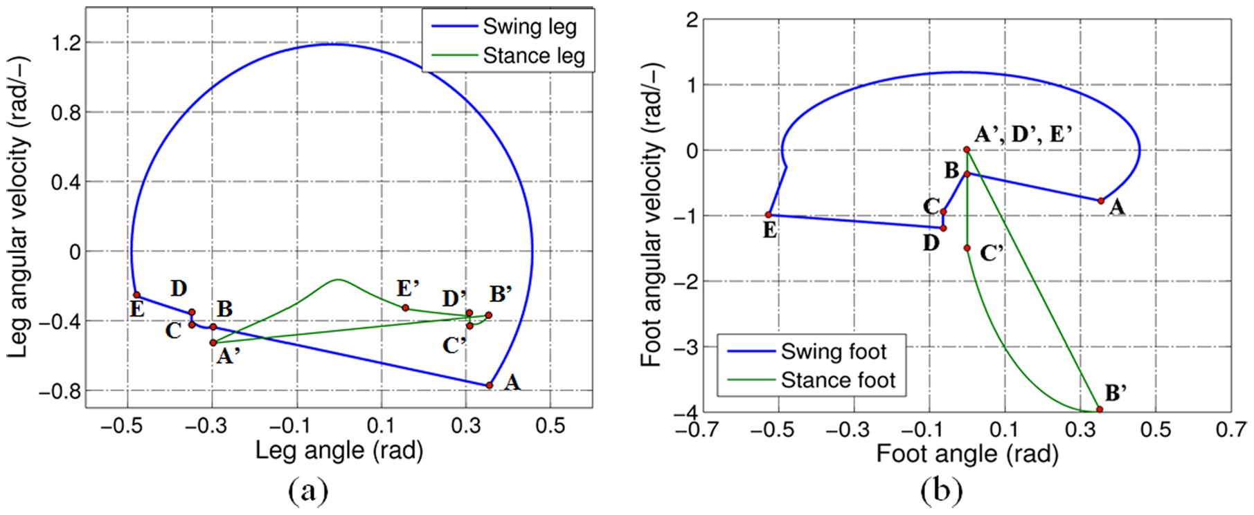
(a) Limit cycles of the swing and stance legs and (b) Limit cycles of the swing and stance feet.

The two legs of the walking model show two limit cycles during walking which implies that the model can converge to its initial condition for every step. From points A to E and points A′ to E′, the model walks stably from the first impact phase to the swing phase.

The two feet of the walking model show two limit cycles as well, as shown in Figure 6(b). From points A to E and points A′ to E′, the model walks stably from the first impact phase to the swing phase. For the stance (i.e. leading) foot, its angle and angular velocity value is kept at 0 after the second impact phase, so A′, B′, and E′ share the same point.

The stick diagram of the walking process is depicted in Figure 7, in which the robot shows a stable walking with periodical gait.

Figure 7.

Stick diagram of the passive walking model.

The main features for a walking model with flat feet that contains double stance phase in this study are (1) the double stance phase accounts for 25.5% of one step time and (2) there are two times of impact during walking and the second impact has tiny influence on the walking dynamics.

Effect of swing ankle angle’s value on walking performance

Fully passive dynamic biped walking robot

In this section, we introduce the influence of swing ankle angle on walking performance for the fully passive walking model in this study. The walking performance refers to that of walking stability, step length, and step duration.

We try to change the swing ankle angle before first impact based on the following equation

θ_{3}^{-} = θ_{1}^{-} + θ_{w}^{-} \cdot \frac{π}{180}

(26)

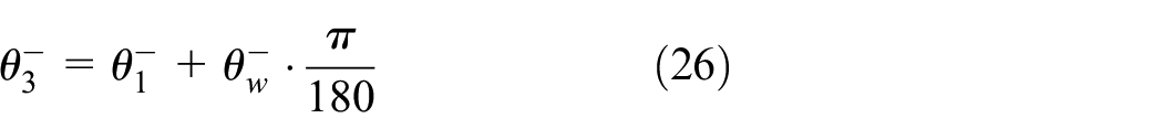
The value of the ankle joint angle $θ_{w}$ is set immediately to a value and kept constant during the swing phase by the last constraint function listed in equation (20) at the start of the swing phase in simulation, which means that the control of this joint is finished immediately. However, in practice, the change in the ankle joint angle should be realized by an active controlled spring that is connected to a motor.

When $θ_{w}^{-} = 0$ , the ankle is in its equilibrium position. So we change the value for $θ_{w}^{-}$ in a reasonable range and try to obtain the fixed point for different ankle angle first. We also consider that the results can be varied greatly with the change of the hinder-foot length, so we change the hinder-foot length from 0.05 to 0.1 to investigate this effect.

Figure 8 shows the difference of the two limit cycles for the swing ankle angle at −15°and 35°, respectively. From points A to E and points A′ to E′, the model walks successfully from the first impact phase to the swing phase. Figure 9 shows the influence of different ankle angle values on walking stability under different hinder-foot lengths.

Figure 8.

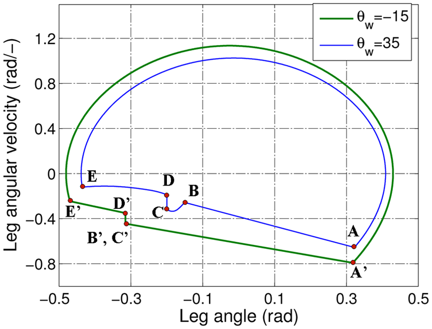
Limit cycles under different swing ankle angles.

Figure 9.

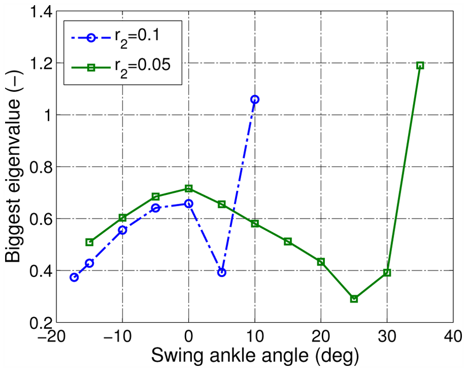
Walking stability under different swing ankle angles.

In Figure 8, we found that the limit cycles under different swing ankle angle values are quite different which implies that the change in ankle angle value has an obvious influence on the walking performance. When $θ_{w}^{-} = - 15$ , we can hardly find the first double stance phase which implies that the swing foot is nearly parallel to the walking surface at the instant just before first impact. We cannot find the fixed point when the swing ankle angle is smaller than −17.7 or bigger than 38 when the hinder-foot length is equal to 0.05, and we cannot find the fixed point when the swing ankle angle is smaller than −17 or bigger than 10 when the hinder-foot length is equal to 0.1.

Figure 9 shows the biggest eigenvalues of the Jacobian matrix for the Poincare mapping function under different ankle angle values which can be used as a criterion to determine whether the passive robot is locally stable. When the biggest eigenvalue is smaller than 1, we deem that the robot is locally stable. Analytical solution for the Jacobian matrix is extremely hard to obtain, so we obtain the Jacobian matrix based on the numerical method as described in Kim et al.³¹ We take the module of the biggest eigenvalue if it is a plural. From the figure, we can see that the robot is getting more stable when the ankle angle value is changed from its equilibrium position in most area within the changing range. When the hinder-foot length is equal to 0.1, this influence is more obvious. In general, the different ankle angle values can affect the walking stability greatly which means that we can obtain a better walking stability by just changing the swing ankle angle before impact.

Figure 10 shows the effect of different swing ankle angle values on step length under different hinder-foot lengths. Figure 11 shows the effect of different swing ankle angle values on step duration under different hinder-foot lengths.

Figure 10.

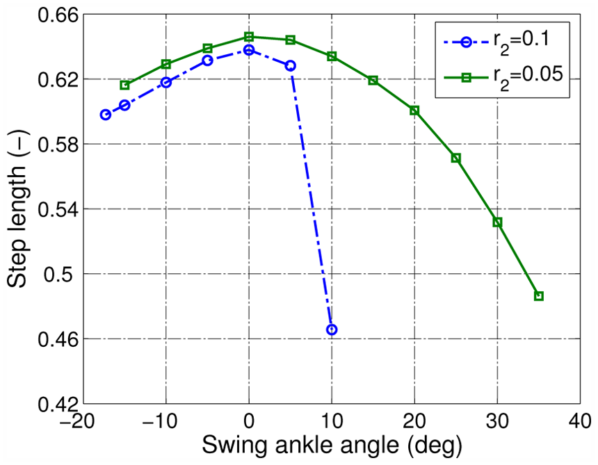
Step length under different swing ankle angles.

Figure 11.

Step duration under different swing ankle angles.

The step length is calculated as follows

L = l_{f} + l \cdot \sin (θ_{1}^{+}) - l_{f 2} \cdot \cos (θ_{3}^{+}) - l \cdot \sin (θ_{2}^{+}) - l_{f 1} \cdot \cos (θ_{4}^{+})

(27)

In equation (27), $θ^{+}$ means the instant just after first impact. From Figure 10, we can see that the step length changes slowly when the swing ankle angle is smaller than 0 and changes rapidly when it is bigger than 0. The step length can be changed from 0.64604 to 0.48622, which is about 25% of its initial value. So we can change the step length by only changing the swing ankle angle before impact. When the hinder-foot length is equal to 0.1, this change happens rapidly.

In Figure 11, we can see that the step duration changes slowly when the swing ankle angle is smaller than 5 and changes rapidly when it is bigger than 5. The step duration can be changed from 2.1864 to 3.6473, which is about 66.8% of its initial value. When the hinder-foot length is equal to 0.1, this change is more obviously, which is about 94.4% of its initial value. So the changing of swing ankle angle has a great influence on the step duration. In other words, the changing of swing ankle angle value has a great influence on the walking speed.

In general, we can change the walking stability, step length, and step duration by just changing the swing ankle angle before first impact, especially when we want a smaller step length and a slower walking speed. It should be mention that the changing of the walking performance is mainly caused by the change in of the fixed point which is caused by the change in of the swing ankle angle (i.e. changing of the swing ankle angle is the direct factor but changing of the fixed point is the primary factor).

Quasi-passive dynamic walking robot

For a quasi-passive dynamic walking robot prototype, it is extremely hard to obtain the fixed point in the experiments as the passive robot is usually initialed manually. So it is hard to compute the biggest eigenvalues of the Jacobian matrix in experiments. In practice, the step length or step duration (i.e. walking velocity) is usually used as the criterion to determine whether the robot is walking stably, like the gait sensitivity norm³² criterion. If the robot has nearly the same step length or step duration for every step, it is considered that the walking is stable. Humans try to keep the walking balance by changing the step length or step duration,³³ and usually a faster walking speed needs a bigger step length and vice versa.³³

So in this section, we try to investigate whether we can adjust the step duration of the next step by only changing the swing ankle angle before impact. We investigate this by observing the amount of total kinetic energy of the robot before impact and the amount of lost kinetic energy during impact. More remained kinetic energy after impact implies a higher initial walking speed (i.e. less walking duration) of the next step and vice versa. The kinetic energy can be calculated based on the following equation

\begin{array}{l} E = \frac{m_{l} (v_{c 1}^{2} + v_{c 2}^{2})}{2} + \frac{m_{h} \cdot v_{h}^{2}}{2} + \frac{m_{f} (v_{c f 1}^{2} + v_{c f 2}^{2})}{2} \\ + \frac{J_{l} (θ_{1}^{2} + θ_{2}^{2})}{2} + \frac{J_{f} (θ_{3}^{2} + θ_{4}^{2})}{2} \end{array}

(28)

We also use the passive walking model here to make the analysis, but we give the same initial condition for one walking step with different swing ankle angle values. This can guarantee that the change in the walking performance is only caused by the change in the ankle angle.

Figure 12(a) shows the total kinetic energy change under different swing ankle angle values when the slope angle value is equal to 3°. In Figure 12(a), the top block denotes the kinetic energy before first impact and the bottom block denotes the remained kinetic energy after impact. The vertical line denotes the amount of the lost kinetic energy during impact, which means that the longer the line the more kinetic energy lost in the impact.

Figure 12.

(a) Changing of the kinetic energy of the robot when the slope angle is equal to 3 (degree) and (b) Changing of the kinetic energy of the robot when the slope angle is equal to 5 (degree).

From the figure, we found that when the swing ankle angle is getting bigger before impact, the amount of total kinetic energy before impact is getting smaller. When the swing ankle angle is getting bigger before impact, the amount of lost kinetic energy during impact is getting bigger. So the amount of remained kinetic energy for the next step is getting smaller with the increase in the swing ankle angle before impact. The amount of remained kinetic energy after impact can be reduced from 0.0690 to 0.0512, about 25.8% of its initial value when the swing ankle angle changes from 0 to 35, and can be enhanced from 0.0690 to 0.0766, about 9.9% of its initial value when the swing ankle angle changes from 0 to −15. There are two main reasons for this effect: (1) the increase in the swing ankle angle value makes the swing heel impact with the ground at an earlier time, which decrease the angular velocity of each part of the robot and thus the amount of kinetic energy and (2) the increase in the swing ankle angle value changes the impact posture of the robot, which influence the amount of lost kinetic energy during impact. So we can obtain a more proper initial walking speed of the next step by just simply changing the swing ankle angle, especially when the walking speed of this step is too fast. This can thus enhance the walking stability of the next step.

We also want to investigate how the changing of the swing ankle angle can influence the initial walking speed of the next step when the walking is faster. So we change the slope angle from 3°to 5° which can give a higher speed of the walking. The bigger slope angle value has the same effect with a bigger driving torque. As shown in Figure 12(b), the remained kinetic energy changes more than that under the slope angle value of 3°. The remained kinetic energy can be reduced from 0.0957 to 0.0624, which means that when the robot is walking faster the influence is getting bigger.

In Hobbelen and Wisse,²¹ the authors adjust the walking speed by adjusting the amount of ankle push-off torque. This is more effective when the walking is too slow. In Hobbelen and Wisse,²⁵ the authors adjust the initial walking speed of the next step by “swing leg retraction,” which is an effective way to get better walking stability of the next step. However, changing the state of the swing leg costs more energy than changing the state of the swing ankle angle as the mass of the foot is much lower than the leg. Our method also provides a way to adjust the initial walking speed of the next step but with low energy consumption. And the method is more effective when the walking is too fast, which is a complementary method to that in Hobbelen and Wisse,²¹ so combining the method in Hobbelen and Wisse²¹ and in this article may obtain a better walking stability to resist disturbances during walking.

Conclusion

In this article, a passive walking model that consisted of two straight legs, two flat feet, two ankle joints, and a hip joint was built. A detailed walking dynamics was derived which contains double stance phase that makes the walking gait more natural. The instant just before impact is chosen as the initial condition for the walking, which reduces the number of the independent initial state variables from 5 to 3. The main features for a walking model with flat feet that contains double stance phase in this study is that (1) the double stance phase accounts for 25.5% of one step time and (2) there are two times of impact during walking and the second impact has tiny influence on the walking dynamics.

A detailed analysis based on the numerical simulation for the influence of the swing ankle angle on the walking performance was introduced. For a fully passive walking robot, we can obtain a better walking stability in a reasonable range when changing the swing ankle angle from its equilibrium position. The step length could be changed about 25% and the step duration could be changed about 66.8% by just changing the swing ankle angle before first impact. A bigger swing ankle angle will lead to a lower initial walking speed of the next step. When the swing hinder-foot length is getting bigger, this influence is getting bigger.

When it comes to the quasi-passive dynamic walking robot, we can reduce the amount of remained kinetic energy after impact about 25.8% when the swing ankle angle changes from 0 to 35 and enhance that about 9.9% when the swing ankle angle changes from 0 to −15. So we can obtain a more proper initial walking speed of the next step by just simply changing the swing ankle angle, especially when the walking speed of this step is too high. Thus, this might enhance the walking stability of next step when the robot has encountered disturbances that cause speed change of this step. When the robot is walking faster, this influence is getting bigger.

Footnotes

Academic Editor: Mario L Ferrari

Declaration of conflicting interests

The author(s) declared no potential conflicts of interest with respect to the research, authorship, and/or publication of this article.

Funding

The author(s) disclosed receipt of the following financial support for the research, authorship, and/or publication of this article: This research is funded and supported by National Magnetic Confinement Fusion Science Program “Multi-Purpose Remote Handling System with Large-Scale Heavy Load Arm” (2012GB102004).

References

Sakagami

Watanabe

Aoyama

. The intelligent ASIMO: system overview and integration. In: IEEE/RSJ international conference on intelligent robots and systems, Lausanne, 30 September–4 October 2002, vol. 3, pp.2478–2483. New York: IEEE.

Strom

Slavov

Chown

. Omnidirectional walking using ZMP and preview control for the NAO humanoid robot. In: Baltes

Lagoudakis

Naruse

. (eds) RoboCup 2009: robot soccer world cup XIII. Berlin, Heidelberg: Springer, 2010, pp.378–389.

Collins

Ruina

A bipedal walking robot with efficient and human-like gait. In: Proceedings of the 2005 IEEE international conference on robotics and automation, ICRA’05, Barcelona, 18–22 April 2005, pp.1983–1988. New York: IEEE.

Kajita

Kanehiro

Kaneko

. Biped walking pattern generation by using preview control of zero-moment point. In: Proceedings of the ICRA’03 IEEE international conference on robotics and automation, Taipei, Taiwan, 14–19 September 2003, vol. 2, pp.1620–1626. New York: IEEE.

McGeer

Passive dynamic walking. Int J Robot Res 1990; 9: 62–82.

McGeer

. Passive walking with knees. In: Proceedings of the 1990 IEEE international conference on robotics and automation, Cincinnati, OH, 13–18 May 1990, pp.1640–1645. New York: IEEE.

Collins

Ruina

Tedrake

. Efficient bipedal robots based on passive-dynamic walkers. Science 2005; 307: 1082–1085.

Hobbelen

De Boer

Wisse

. System overview of bipedal robots flame and tulip: tailor-made for limit cycle walking. In: IEEE/RSJ international conference on intelligent robots and systems, IROS’08, Nice, 22–26 September 2008, pp.2486–2491. New York: IEEE.

Schuitema

Hobbelen

DGE

Jonker

. Using a controller based on reinforcement learning for a passive dynamic walking robot. In: 5th IEEE-RAS international conference on humanoid robots, Tsukuba, Japan, 5 December 2005, pp.232–237. New York: IEEE.

10.

Wisse

Hobbelen

DGE

Rotteveel

RJJ

. Ankle springs instead of arc-shaped feet for passive dynamic walkers. In: 6th IEEE-RAS international conference on humanoid robots, Genova, 4–6 December 2006, pp.110–116. New York: IEEE.

11.

Narukawa

Yokoyama

Takahashi

. A simple 3D straight-legged passive walker with flat feet and ankle springs. In: IEEE/RSJ international conference on intelligent robots and systems, IROS’08, Nice, 22–26 September 2008, pp.2952–2957. New York: IEEE.

12.

Wisse

Hobbelen

DGE

Schwab

AL.

Adding an upper body to passive dynamic walking robots by means of a bisecting hip mechanism. IEEE T Robot 2007; 23: 112–123.

13.

Hass

Herrmann

Geisel

Optimal mass distribution for passivity-based bipedal robots. Int J Robot Res 2006; 25: 1087–1098.

14.

Schwab

Wisse

. Basin of attraction of the simplest walking model. In: Proceedings of the ASME design engineering technical conferences and computers and information in engineering conference, Pittsburgh, Pennsylvania, 9–12 September, vol. 6, pp.531–539. New York: ASME.

15.

Huang

Wang

Xie

. Optimal mass distribution for a passive dynamic biped with upper body considering speed, efficiency and stability. In: 8th IEEE-RAS international conference on humanoid robots, Daejeon, South Korea, 1–3 December 2008, pp.515–520. New York: IEEE.

16.

Hsu

CS.

Global analysis by cell mapping. Int J Bifurcat Chaos 1992; 2: 727–771.

17.

Collins

Wisse

Ruina

A three-dimensional passive-dynamic walking robot with two legs and knees. Int J Robot Res 2001; 20: 607–615.

18.

Westervelt

Grizzle

Koditschek

DE.

Hybrid zero dynamics of planar biped walkers. IEEE T Automat Contr 2003; 48: 42–56.

19.

Chevallereau

Gabriel

Aoustin

. Rabbit: a test bed for advanced control theory. IEEE Contr Syst Mag 2003; 23: 57–79.

20.

Wisse

Schwab

Van der Linde

. How to keep from falling forward: elementary swing leg action for passive dynamic walkers. IEEE T Robot 2005; 21: 393–401.

21.

Hobbelen

DGE

Wisse

. Ankle actuation for limit cycle walkers. Int J Robot Res 2008; 27: 709–735.

22.

Hobbelen

DGE

Wisse

. Controlling the walking speed in limit cycle walking. Int J Robot Res 2008; 27: 989–1005.

23.

Spong

Holm

Lee

Passivity-based control of bipedal locomotion. IEEE Robot Autom Mag 2007; 14: 30–40.

24.

Hürmüzlü

Moskowitz

GD.

The role of impact in the stability of bipedal locomotion. Dynam Stabil Syst 1986; 1: 217–234.

25.

Hobbelen

DGE

Wisse

. Swing-leg retraction for limit cycle walkers improves disturbance rejection. IEEE T Robot 2008; 24: 377–389.

26.

Huang

Wang

Gao

. Modeling and analysis of passive dynamic bipedal walking with segmented feet and compliant joints. Acta Mech Sinica 2012; 28: 1457–1465.

27.

Ruina

Bertram

JEA

Srinivasan

A collisional model of the energetic cost of support work qualitatively explains leg sequencing in walking and galloping, pseudo-elastic leg behavior in running and the walk-to-run transition. J Theor Biol 2005; 237: 170–192.

28.

Goswami

Thuilot

Espiau

Compass-like biped robot part I: stability and bifurcation of passive gaits. INRIA research report no. 2996, October 1996.

29.

Spong

Hutchinson

Vidyasagar

Robot modeling and control. New York: Wiley, 2006.

30.

Duindam

Port-based modeling and control for efficient bipedal walking robots, 2006, http://bibtexbib.free.fr/bibliographie_net/duindam_phdthesis.pdf

31.

Kim

Choi

Spong

MW.

Passive dynamic walking with knee and fixed flat feet. In: IEEE international conference on systems, man, and cybernetics (SMC), Seoul, South Korea, 14–17 October 2012, pp.2744–2750. New York: IEEE.

32.

Hobbelen

DGE

Wisse

. A disturbance rejection measure for limit cycle walkers: the gait sensitivity norm. IEEE T Robot 2007; 23: 1213–1224.

33.

Kuo

AD.

A simple model of bipedal walking predicts the preferred speed–step length relationship. J Biomech Eng 2001; 123: 264–269.

Influence of the swing ankle angle on walking stability for a passive dynamic walking robot with flat feet

Abstract

Keywords

Introduction

Walking dynamics

Walking phases

Phase a: First impact phase

Phase b: First double stance phase

Phase c: Second impact phase

Phase d: Second double stance phase

Phase e: Swing phase

Walking dynamics

First impact phase

First double stance phase

Second impact phase

Second double stance phase

Swing phase

Numerical simulation and results

Numerical simulation process

Simulation results

Effect of swing ankle angle’s value on walking performance

Fully passive dynamic biped walking robot

Quasi-passive dynamic walking robot

Conclusion

Footnotes

Declaration of conflicting interests

Funding

References