Sage Journals: Discover world-class research

Abstract

The concept of “passive dynamic walking robot” refers to the robot that can walk down a shallow slope stably without any actuation and control which shows a limit cycle during walking. By adding actuation at some joints, the passive dynamic walking robot can walk stably on level ground and exhibit more versatile gaits than fully passive robot, namely, the “limit cycle walker.” In this article, we present the mechanical structures and control system design for a passive dynamic walking robot with series elastic actuators at hip joint and ankle joints. We built a walking model that consisted of an upper body, knee joints, and flat feet and derived its walking dynamics that involve double stance phases in a walking cycle based on virtual power principle. The instant just before impact was chosen as the start of one step to reduce the number of independent state variables. A numerical simulation was implemented by using MATLAB, in which the proposed passive dynamic walking model could walk stably down a shallow slope, which proves that the derived walking dynamics are correct. A physical passive robot prototype was built finally, and the experiment results show that by only simple control scheme the passive dynamic robot could walk stably on level ground.

Keywords

Passive dynamic walking biped robot walking dynamics mechanical structure control system series elastic actuators

Introduction

Humans can walk so well on ground that they walk with natural gait (inverted pendulum-like gait), low energy consumption, high stability and great versatility. To study and simulate human walking, numerous robots have been built recently. The traditional biped walking robot, such as the famous Asimo¹ and HRP-2,² can walk stably with very versatile gaits such as hopping, climbing stairs, changing walking direction or even walking on rough terrains. However, because the main control schemes are based on the zero moment point (ZMP) method, by which all joints must be controlled at every instant to keep the ZMP within the convex hull of the feet to reach static equilibrium all the time, the walking energy consumption is high³ and the walking gaits are quite unnatural. The concept of “passive dynamic walking,” first proposed by McGeer,⁴ gives out a new way to build bipedal walking robot. Biped walking robots built based on this concept can walk down a shallow slope stably by making use of their own dynamics if specific physical parameters and a proper initial condition are given. So they can walk with human-like gaits and consume low energy when walking. However, the walking stability is low and walking gaits are not versatile. So the passive dynamic walking robots with more complex mechanical structures were built. McGeer⁵ first built a passive dynamic walker with the knee joints and curved feet. Passive dynamic walking was first extended to three dimensions in Collins et al.⁶

To make the robot walk on level ground, actuations must be added to some joints of the robot, namely, “limit cycle walking.”⁷ Recently, some successful limit cycle walkers have been built by researchers,^8–10 ranging from motor driving to pneumatic driving or from hip actuation to ankle actuation.

In previous research, some researchers built the passive robot with point feet or curved feet and assumed that only single stance phase exists during walking. However, like humans, flat feet play an important role during walking and double stance phase (i.e. both feet contact with ground at one time) exists during walking.¹¹ M Wisse and DGE Hobbelen¹² prove that flat feet perform better than curved feet for passive walking robot. Flat feet were extended to segmented flat feet in Huang et al.,¹³ and double stance phase walking dynamics were studied by a simple walking model.

In this study, we designed and built a passive dynamic walking robot with series elastic actuators (SEA)¹⁴ at both hip joint and ankle joints. We derived the walking dynamics with double stance phases for the walking model that consisted of an upper body, knee joints, ankle joints, and flat feet by virtual power principle.¹⁵ We validated the correctness of the walking dynamics by numerical simulations in MATLAB. A physical passive robot prototype was built and the experimental results show that the passive dynamic walking robot designed in this study could walk stably on level ground.

The article is organized as follows. In section “Mechanical structure design process,” the mechanical structure design process of the passive dynamic walking robot is proposed. The control system architecture is introduced in section “Control system architecture.” Walking dynamics is derived in section “Walking phases and walking dynamics.” Numerical simulation process is introduced and the experiment results are given in section “Numerical simulation and experiments.” We conclude in section “Conclusion.”

Mechanical structure design process

Overall design

A passive dynamic walking robot that consisted of an upper body, a hip joint, two knee joints, two ankle joints, and two flat feet was designed in this study as depicted in Figure 1. Each two legs are fixed together to form one leg which constrains the robot walking in the sagittal plane. It has 6 degrees of freedom (DOF), two located at hip joints, two at knee joints, and two at ankle joints. The upper body is constrained by a bisecting mechanism,¹⁶ which can passively keep the torso in the midway between the two legs all the time without adding extra DOF to the passive robot.

Figure 1.

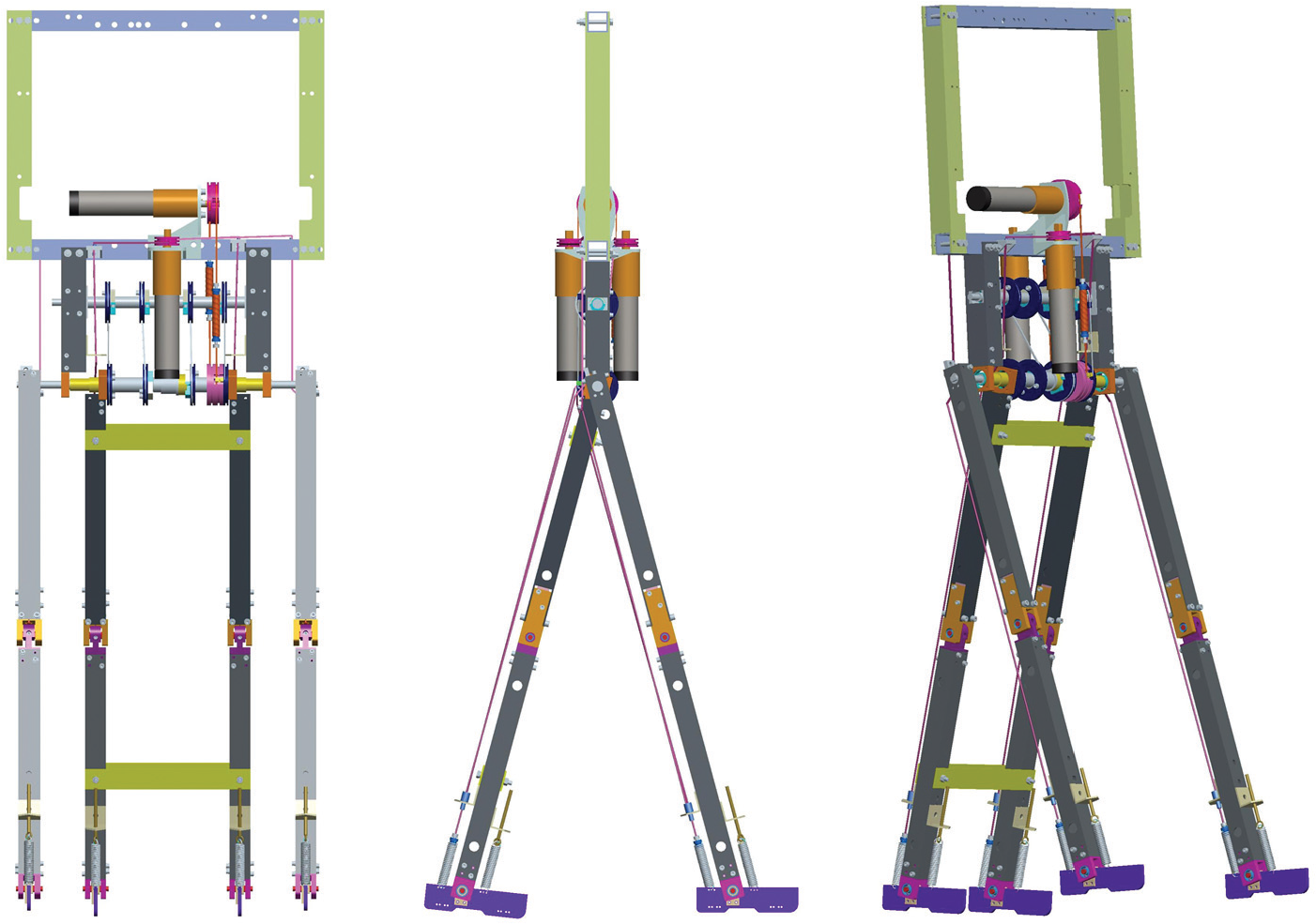
Pro/E model of the passive dynamic walking robot.

Upper body and SEA design

As mentioned above, the upper body is constrained by a bisecting mechanism to keep itself in the midway between the two legs all the time, as shown in Figure 2. The bisecting mechanism is consisted of eight constraint wheels, and two of them are installed at the output shaft, two of them are fixed at the top of the inner leg, while the other four are installed at the auxiliary shaft. Four of them form two opposite “S” types and the other four form two opposite “C” types through steel-wire cables. So when the inner leg rotates to one direction, the outer leg will rotate the same angle to the opposite direction through the eight constraint wheels which will keep the upper body in the midway of the two legs all the time.

Figure 2.

Upper body of the passive dynamic walking robot.

Three direct current (DC) motors are installed on the upper body, one is used to actuate the hip joint and the other two are used to actuate the two ankle joints. They are connected to each actuated joint through spring and steel-wire cables which forms the SEA. The compliant actuation is quite essential for a passive dynamic robot, because the passive robot moves largely relying on their natural dynamics.¹⁷ The high compliance of the compliant actuation provides the possibility to make use of the robot’s own dynamics. By controlling the elongation of the spring, we can convert the force control into position control for the joints.

The steel-wire cables are connected to the springs by using a screw bolt (the blue part) and a screw (the gray part), as depicted in Figure 2. The screw bolt can adjust the spring’s effective length to adjust its stiffness by screw itself in or out of the spring. The screws are used to adjust the preload of the steel-wire cables.

Knee joint design

To avoid foot-ground scuffing, knee joints are added to our passive robot. The knee should be locked when the leg rotates forward as the stance leg and unlock itself when the leg swings forward as the swing leg as well. So, we use electromagnet to drive a taper pin to lock and release the knee joint. The electromagnet and taper pin are installed on the thigh and a taper pin-hole is at the top of the shank, as shown in Figure 3. The taper shape fit can remove the fit clearance to avoid the knee bending when locked. The knee can be locked by itself with the rotation of the shank and unlocked by the electromagnet. An extra limiting surface is designed to prevent the knee joint from over-bending.

Figure 3.

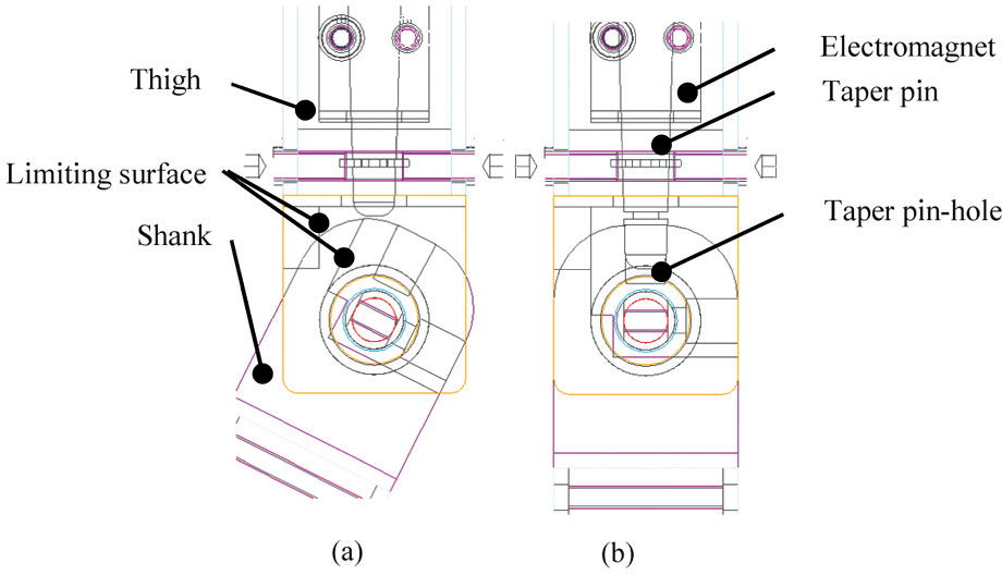
(a) Unlocked and (b) locked states of the knee joint.

Ankle joint design

Ankle compliance is added by installing two antagonistic-connected springs. One is connected to the motor installed on the upper body to form an SEA and the other one is connected to an adjusting bolt that can adjust the preload force of the spring, as depicted in Figure 4.

Figure 4.

Ankle joint.

Control system architecture

The hardware of the control system is built based on a distributed architecture, as shown in Figure 5. All control is performed on PC by lines of C++ codes. The PC is used to plan joint motions, coordinate joint motions, and send movement orders to the DC motor’s digital signal processor (DSP) controller via controller area network (CAN) bus. We use ACK-055-06 (a digital servo amplifier from Copley Corporation) to drive each actuated joint, perform the local joint feedback control, read joint encoder data, and send it back to the PC. We use PCI1784 (a universal PCI card from Advantech Corporation) card to read control input data consisted of encoder data from the encoder located at the auxiliary shaft and ankle joints and foot contact switches under the feet via PCI bus. The PCI card is also used to drive relays to lock and release the electromagnets at the knee joints.

Figure 5.

Architecture of the control system.

The basis of the PC controller is an event-based state machine. One control loop can be divided into “heel impact,”“double stance,”“single stance, inner leg swing,” and “single stance, outer leg swing” phases. The event that triggers the system state from one to another is the detection of each micro switch’s state under each foot.

Walking phases and walking dynamics

Walking phases

The walking dynamics for the passive dynamic walking robot is the basis for analyzing the walking stability and simulating the control, so we derive the walking dynamics in this section.

The walking phases for one walking step can be divided into “first foot-ground impact,”“first double stance,”“second foot-ground impact,”“second double stance,”“four-link swing,”“knee impact,” and “three-link swing” phases, as shown in Figure 6.

Figure 6.

Walking phases in one walking step.

Phase a: first foot-ground impact

The swing foot’s heel impacts with the ground for the first time and thus becomes the new stance leg. This phase is the start of a passive walking step. Usually, the state after foot-ground impact is chosen to be the start of one step, but in this article, to decrease the number of independent initial condition parameters, we choose the instant just before foot-ground impact as the start of one step.

Phase b: first double stance

Both the leading leg and trailing leg’s feet keep contact with the ground, and the legs rotate forward together. The leading leg rotates around the heel, and which part of the foot the trailing leg rotates around depends on the contact force under the foot.

Phase c: second foot-ground impact

The leading foot’s toe impacts with the ground which leads to a full contact of the leading foot with the ground.

Phase d: second double stance

The leading leg and trailing leg’s feet are still in contact with the ground and rotate forward together. The leading leg rotates around the ankle joint, and the trailing leg rotates around the foot–toe contact point.

Phase e: four-link swing phase

The trailing leg has lost contact with the ground and becomes the new swing leg. The knee joint of the swing leg is released at the start of this phase, and thus the model becomes the four-link model.

Phase f: knee impact

When the shank of the swing leg has rotated to the limiting position, the knee joint impacts, and the swing leg becomes one straight leg.

Phase g: three-link swing phase

The walking model becomes the three-link model as the knee joint has been locked. The swing leg keeps swinging forward until its heel impacts with the ground again. By now, one cycle of walking is ended.

Walking dynamics

A walking model that consisted of an upper body, a hip joint, knee joints, ankle joints, and flat feet is built in this study, as shown in Figure 7.

Figure 7.

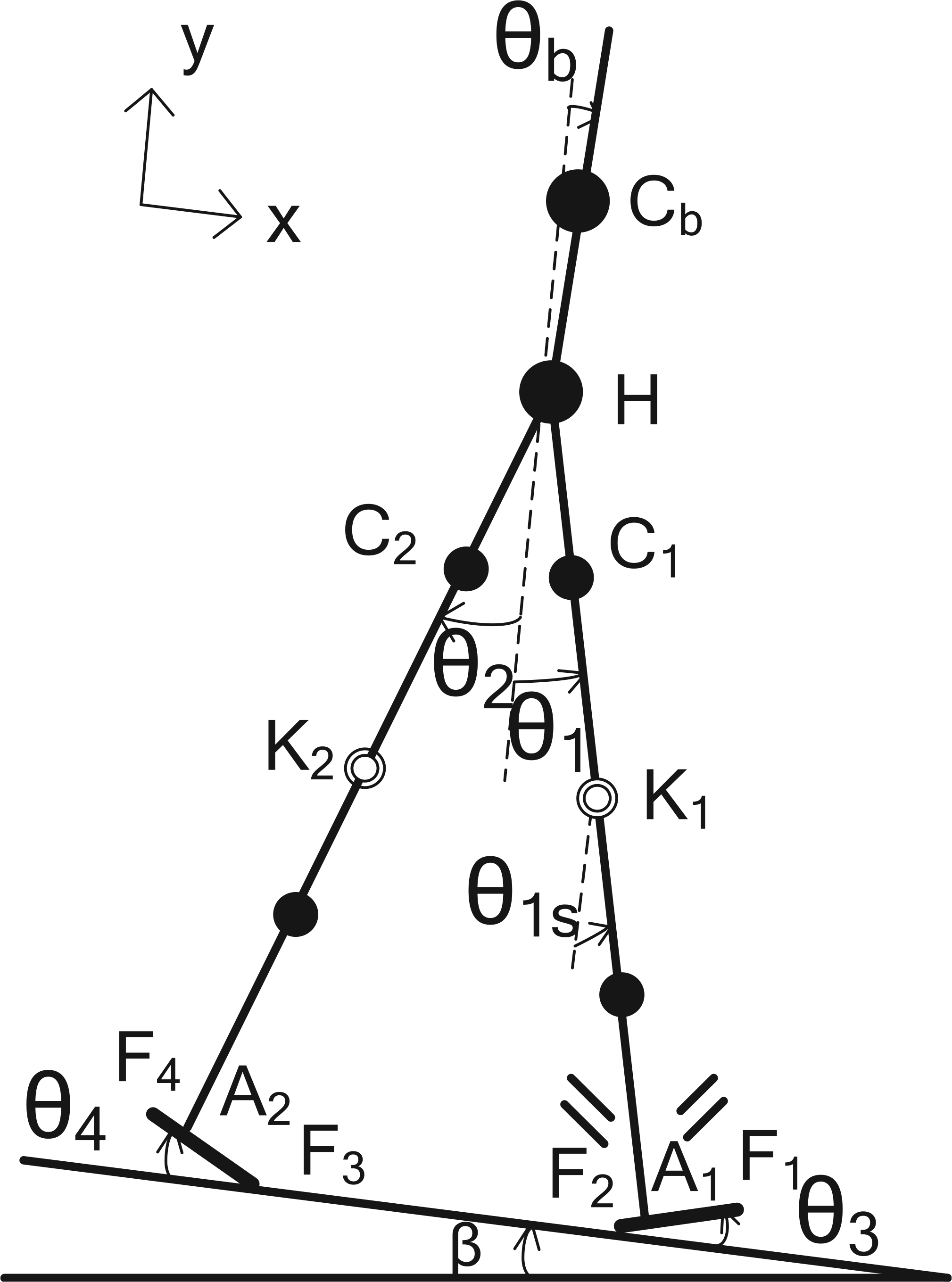
Passive dynamic walking model.

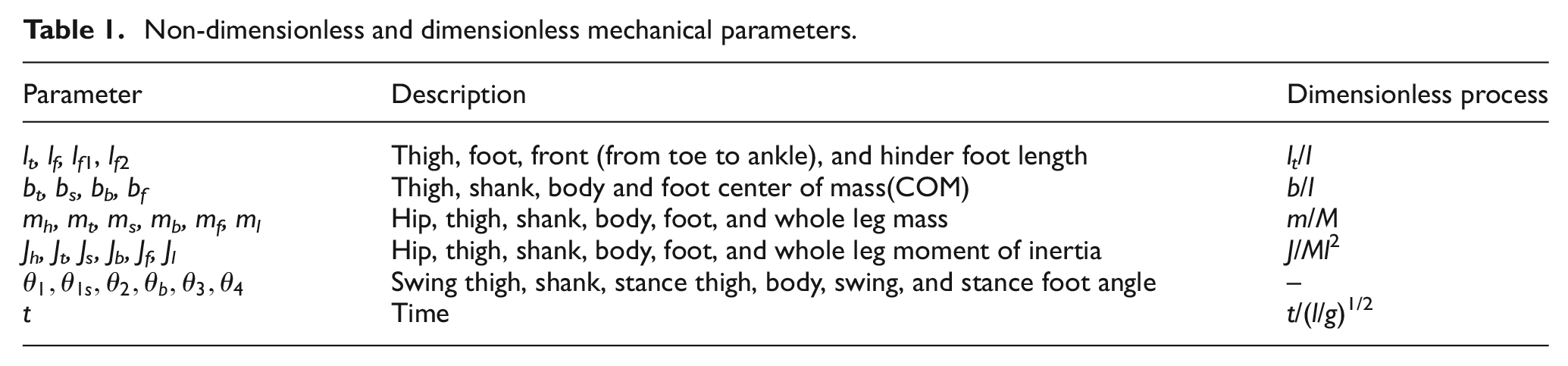
The mechanical parameters and the dimensionless form are shown in Table 1. Dividing the parameters by leg length l or total mass of the robot M, all parameters can be turned into dimensionless form, for the reason of easier calculating and comparability.

Table 1.

Non-dimensionless and dimensionless mechanical parameters.

Parameter	Description	Dimensionless process
l_t, l_f, l_f ₁, l_f ₂	Thigh, foot, front (from toe to ankle), and hinder foot length	l_t /l
b_t, b_s, b_b, b_f	Thigh, shank, body and foot center of mass(COM)	b/l
m_h, m_t, m_s, m_b, m_f, m_l	Hip, thigh, shank, body, foot, and whole leg mass	m/M
J_h, J_t, J_s, J_b, J_f, J_l	Hip, thigh, shank, body, foot, and whole leg moment of inertia	J/Ml ²
$θ_{1}, θ_{1 s}, θ_{2}, θ_{b}, θ_{3}, θ_{4}$	Swing thigh, shank, stance thigh, body, swing, and stance foot angle	–
t	Time	t/(l/g)^1/2

Usually, the Poincare mapping method¹⁸ is used to describe the periodic walking and analyze the local stability of a passive robot. By choosing a Poincare section through which the walking trajectory passes periodically, we can set the initial condition obtained from the state just on the Poincare section for the walking. If the robot can converge to the same initial condition after one or few steps, we can consider that the walking is stable, and the converged initial condition is called the fixed point.¹⁸

To make the walking dynamics easier to calculate, the state just after foot strike is chosen as the Poincare section typically. However, in this article, we choose the instant just before foot-ground impact as the Poincare section (i.e. initial condition). By this way, the independent state variables can be reduced to three, which are $θ_{1}, {\overset{\cdot}{θ}}_{1}$ , and ${\overset{\cdot}{θ}}_{2}$ , as shown in equations (1)–(3). In equation (1), $θ^{-}$ denotes the joint angle value just before impact, and $θ_{sf}$ denotes the angle between the shank and the foot. In this article, $θ_{sf}$ is set to $π / 2$ throughout the swing phase, which means that during the swing phase, the foot is always kept perpendicular to the shank. Equation (2) is induced by the bisecting mechanism. If the ankle joint stiffness is too big, there will be a pre-mature heel rise at the stance heel before impact which leads to an unnatural oscillatory ankle motion as discussed in Hobbelen and Wisse.¹⁰ So, we assume that the stance foot keeps full contact with the ground before the swing heel touches the ground as in equation (3)

{\begin{matrix} θ_{2}^{-} = - \arccos (\frac{l_{f 1} \cdot \sin θ_{3}^{-} + l \cdot \cos θ_{_{1}}^{-}}{l}) \\ θ_{3}^{-} = θ_{_{sf}}^{-} + θ_{1}^{-} - \frac{π}{2} \\ {\overset{\cdot}{θ}}_{_{3}}^{-} = {\overset{\cdot}{θ}}_{_{1}}^{-} \end{matrix}

(1)

θ_{b} = \frac{θ_{1} + θ_{2}}{2}

(2)

θ_{_{4}}^{-} = {\overset{\cdot}{θ}}_{_{4}}^{-} = 0

(3)

1. First foot-ground impact.

During this phase, we assume that the foot-ground impact is handled as instantaneous and fully inelastic impact in which no bounces or slips happen; the joint angles cannot change at that moment. Because the impact happens suddenly, we can ignore the influence of the gravities. So according to the angular momentum theorem, the angular momentum of the entire robot is conserved around the impact point F₂ during impact. The angular momentum of the trailing foot, trailing leg, hip, the leading leg, and upper body is conserved around the leading ankle joint A₁. The angular momentum of the trailing foot, trailing leg, hip, and the upper body is conserved around the hip joint H. The angular momentum of the trailing foot is conserved around the trailing leg ankle joint A₂. The leading leg’s heel joint and trailing legs toe joint should also satisfy the constraint that they must keep contact with the ground during impact as follows

{\begin{matrix} {\overset{\cdot}{x}}_{h}^{+} = {\overset{\cdot}{x}}_{h}^{+} \\ {\overset{\cdot}{y}}_{h}^{+} = {\overset{\cdot}{y}}_{h}^{+} \\ {\overset{\cdot}{θ}}_{b}^{+} = \frac{{\overset{\cdot}{θ}}_{1}^{+} + {\overset{\cdot}{θ}}_{2}^{+}}{2} \\ {\vec{L}}_{F 2}^{+} = {\vec{L}}_{F 2}^{-} + (x_{F 3} - r^{*} - x_{F 2}) \cdot I_{y}^{*} - (y_{F 3} - y_{F 2}) \cdot I_{x}^{*} \\ {\vec{L}}_{A 1} = {\vec{L}}_{A 1} + (x_{F 3} - r^{*} - x_{A 1}) \cdot I_{y}^{*} - (y_{F 3} - y_{A 1}) \cdot I_{x}^{*} \\ {\vec{L}}_{H}^{+} = {\vec{L}}_{H}^{-} + (x_{F 3} - r^{*} - x_{H}) \cdot I_{y}^{*} - (y_{F 3} - y_{H}) \cdot I_{x}^{*} \\ {\vec{L}}_{A 2}^{+} = {\vec{L}}_{A 2}^{-} + (x_{F 3} - r^{*} - x_{A 2}) \cdot I_{y}^{*} - (y_{F 3} - y_{A 2}) \cdot I_{x}^{*} \end{matrix}

(4)

On the left side of the first two equations, we take the trailing leg’s toe-ground contact point F₃ as the origin to calculate ${\overset{\cdot}{x}}_{h}^{+}$ and ${\overset{\cdot}{y}}_{h}^{+}$ . On the right side of the first two equations, we take the leading leg’s heel-ground contact point F₂ as the origin to calculate ${\overset{\cdot}{x}}_{h}^{+}$ and ${\overset{\cdot}{y}}_{h}^{+}$ . This can guarantee the constraint that the trailing leg’s toe and the leading leg’s heel must keep contact with the ground during impact.

Because of the existence of double stance phase, the trailing leg will not lift up immediately and it will still keep contact with the ground, which means that there are impulses both under the leading foot and trailing foot. In equation (4), $I_{x}^{*}$ and $I_{y}^{*}$ denote the component of impulse along the x-axis and y-axis under the trailing foot, respectively. Because we do not actually know the exact position where the impulse generates, we introduce another parameter $r^{*}$ to equation (4), which denotes the distance from the trailing foot’s toe to the exact impulse position. We assume the trailing foot’s heel loses contact with the ground immediately after impact, which means that $r^{*} = 0$ , so there are seven unknown parameters that can be solved by seven equations in equation (4). If $I_{y}^{*} > 0$ , we consider that the assumption above is reasonable. Otherwise, $r^{*} \neq 0$ , which means the trailing foot keeps full contact with the ground during impact. So, ${\overset{\cdot}{θ}}_{4}^{+} = 0$ , and the unknown parameters can also be solved by equation (4).

2. First double stance phase.

During double stance phase, the dynamic system is a nonholonomic one, so the well-known Euler–Lagrange¹⁹ approach is not suitable at this phase. We choose the virtual power¹⁵ approach to derive the walking dynamics in this phase.

The walking dynamics can be described by the rectangular coordinates x and the generalized coordinates q as well, as follows

\begin{matrix} x = [x_{h}, y_{h}, x_{c 1}, y_{c 1}, x_{c 2}, y_{c 2}, x_{cf 1}, y_{cf 1}, x_{cf 2}, y_{cf 2}, x_{cb}, y_{cb}]^{T} \\ q = [x_{h}, y_{h}, θ_{1}, θ_{2}, θ_{3}, θ_{4}, θ_{b}]^{T} \end{matrix}

(5)

In equation (5), two extra redundant coordinates x_h and y_h are added to the generalized coordinates, which will be discussed below.

The rectangular coordinates can be transferred to generalized coordinates as follows

x = x (q)

(6)

Equation (6) can be transferred to the following forms

\begin{matrix} δ \overset{\cdot}{x} = J \cdot δ \overset{\cdot}{q} \\ \overset{\cdot\cdot}{x} = J \cdot \overset{\cdot\cdot}{q} + J' \cdot \overset{\cdot}{q} \end{matrix}

(7)

where $J = \partial x / \partial q$ and $J' = \partial (J \overset{\cdot}{q}) / \partial q$ .

The virtual power approach follows the following form¹⁵ as

δ {\overset{\cdot}{x}}^{T} [f - M \overset{\cdot\cdot}{x}] = 0

(8)

The equation means that for an ideal mass point system, the sum of the virtual power of the active forces and the inertia forces is 0 at any instant, so it can be transferred to the following form as

Δ P + Δ P^{*} = 0

(9)

In equation (9), $Δ P$ denotes the active force’s virtual power, and $Δ P^{*}$ denotes the inertia force’s virtual power. The detailed forms of them are as follows

{\begin{matrix} Δ P = \sum_{i} f_{i} \cdot δ {\overset{\cdot}{x}}_{i} + \sum_{i} τ_{i} \cdot δ {\overset{\cdot}{q}}_{i} \\ Δ P^{*} = - \sum_{i} m_{i} {\overset{\cdot\cdot}{x}}_{i} \cdot δ {\overset{\cdot}{x}}_{i} - \sum_{i} I_{i} {\overset{\cdot\cdot}{q}}_{i} \cdot δ {\overset{\cdot}{q}}_{i} \end{matrix}

(10)

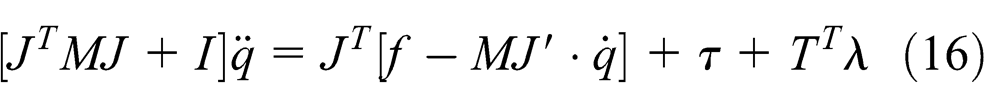
By using equation (7), equation (10) can be transferred to the matrix form based on the generalized coordinates as follows

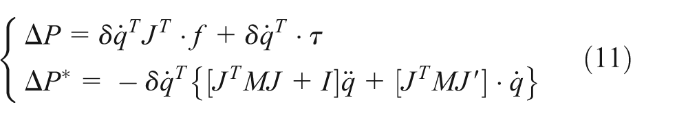
{\begin{matrix} Δ P = δ {\overset{\cdot}{q}}^{T} J^{T} \cdot f + δ {\overset{\cdot}{q}}^{T} \cdot τ \\ Δ P^{*} = - δ {\overset{\cdot}{q}}^{T} {[J^{T} MJ + I] \overset{\cdot\cdot}{q} + [J^{T} MJ'] \cdot \overset{\cdot}{q}} \end{matrix}

(11)

In equation (11), M denotes the mass matrix, I denotes the moment of inertia matrix, f denotes the gravity force matrix, and $τ$ denotes the active force matrix induced by the motors and springs as follows

\begin{matrix} M = Diag (m_{h}, m_{h}, m_{l}, m_{l}, m_{l}, m_{l}, m_{f}, m_{f}, m_{f}, m_{f}, m_{b}, m_{b}) \\ I = Diag (J_{h}, J_{h}, J_{l}, J_{l}, J_{f}, J_{f}, J_{b}) \\ f = Mg [\sin (β), - \cos (β), \sin (β), - \cos (β), \sin (β), \\ - \cos (β), \sin (β), - \cos (β), \sin (β), \\ - \cos (β), \sin (β), - \cos (β)]^{T} \\ τ = [τ_{hx}, τ_{hy}, τ_{sw}, τ_{st}, τ_{f 1}, τ_{f 2}, τ_{b}]^{T} \end{matrix}

(12)

By using equation (11), equation (9) can be transferred to the following form as

δ {\overset{\cdot}{q}}^{T} {J^{T} [f - MJ' \cdot \overset{\cdot}{q}] + τ - [J^{T} MJ + I] \overset{\cdot\cdot}{q}} = 0

(13)

Because the generalized coordinates are not all independent variables, the $λ$ multiplier and the relative constraint must be induced into the system, namely, the Lagrange equation of first kind.¹³

When the trailing foot loses contact with the ground depending on the ground reaction force acting on the foot and the direction of the acceleration of the foot-ground contact point,²⁰ in order to obtain the ground reaction force, at least two extra generalized coordinates $x_{h}$ and $y_{h}$ should be added to the system.

During this phase, the constraint of the system can be described as follows

ε (q) = [\begin{matrix} x_{h} + l \cdot \sin (θ_{1}) + l_{f 1} \cdot \cos (θ_{3}) - l_{f} \\ y_{h} - l \cdot \cos (θ_{1}) + l_{f 1} . \cdot in (θ_{3}) \\ x_{h} + l \cdot \sin (θ_{2}) - l_{f 2} \cdot \cos (θ_{4}) - L \\ y_{h} - l \cdot \cos (θ_{2}) - l_{f 2} \cdot \sin (θ_{4}) \\ θ_{b} - \frac{θ_{1} + θ_{2}}{2} \end{matrix}] = 0

(14)

In equation (14), the trailing leg’s heel-ground contact point F₄ is selected as the origin of the calculation. So the positions of the trailing foot’s toe and leading foot’s heel are l_f and L along the x-axis, respectively. L denotes the step length (from the trailing foot heel-ground contact point to the leading foot heel-ground contact point) here. The first two constraint functions are the trailing foot’s toe position along the x-axis and y-axis, respectively, which implies that the trailing leg’s toe must keep contact with the ground all the time in this phase. The second two constraint functions are the leading foot’s heel position along the x-axis and y-axis, respectively, which implies that the leading foot’s heel must keep contact with the ground all the time in this phase. The last constraint function implies that the upper body is kept in the midway of the two legs all the time, which is induced by the bisecting mechanism discussed above.

Transfer equation (14) into its variational form and multiply by the $λ$ multiplier as follows

δ {\overset{\cdot}{q}}^{T} \cdot T^{T} λ = 0

(15)

In equation (15), $T = \partial ε (q) / \partial q$ , and $λ$ denotes the constraint force induced by each constraint function.

Combining equations (13) and (15), we can obtain the walking dynamics in this phase as follows

[J^{T} MJ + I] \overset{\cdot\cdot}{q} = J^{T} [f - MJ' \cdot \overset{\cdot}{q}] + τ + T^{T} λ

(16)

Equation (14) can be transferred into the following form

T \overset{\cdot\cdot}{q} + (\frac{\partial (T \overset{\cdot}{q})}{\partial q}) \cdot \overset{\cdot}{q} = 0

(17)

Combining equations (16) and (17), we can obtain the walking dynamics that can be solved by using MATLAB as follows

[\begin{matrix} J^{T} MJ - T^{T} \\ T 0 \end{matrix}] [\begin{matrix} \overset{\cdot\cdot}{q} \\ λ \end{matrix}] = [\begin{matrix} J^{T} [f - MJ' \cdot \overset{\cdot}{q}] + τ \\ - (\frac{\partial (T \overset{\cdot}{q})}{\partial q}) \cdot \overset{\cdot}{q} \end{matrix}]

(18)

The walking dynamics in the second foot-ground impact and knee impact phases share the same form with the first foot-ground impact phase. The walking dynamics in the second double stance, four-link swing, and three-link swing phases share the same form with the first double stance phase. Note that the constraint function and walking dynamic parameters are different in different phases. Details of all the coefficient matrixes are omitted due to space limitation.

Numerical simulation and experiments

Numerical simulation

To find stable walking gait and test the walking dynamics derived above, a numerical simulation was performed using MATLAB. The passive robot can walk stably down a gentle slope by providing a proper initial condition to the robot. The proper initial condition here is the so-called fixed point. If in every step the passive walking model is converged to the same initial condition, this initial condition is called the fixed point. The well-known Newton–Raphson iteration algorithm¹⁵ is used to find the fixed point here. The walking phases of a, c, and f are computed on the basis of the principle of angular momentum conservation. The walking phases of b, d, e, and g are integrated numerically by the ODE45 method until the running program detects the impact event of the impact phases. A walking cycle simulation ends before the leading foot’s heel impacts the ground again. The state variables immediately before impact are used as the initial conditions of the next step. If the initial condition converges to one point, the passive walking robot will walk stably with the same gait in every step.

Figure 8 shows the angle values of the legs and upper body for four steps. After the leading foot’s heel impact with the ground, the thigh and shank still rotate forward together for a while, which means that there is a double stance phase existing during this part of walking. The instant that the thigh and shank rotate forward separately is just the time that the trailing foot loses contact with the ground. The upper body is kept strictly in the midway between the two legs, as shown in Figure 8.

Figure 8.

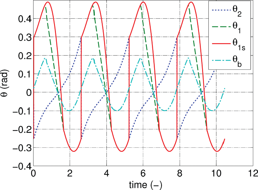
Joint angles for the legs and upper body.

Figure 9 shows the basin of attraction¹⁵ of our passive walking model, which is used to analyze the global stability of the passive robot. The basin of attraction is the collection of all the fixed points (i.e. all the initial conditions that can exhibit a limit cycle during walking) for the walking. The bigger the area of the basin of attraction, the more robust the robot. The basin of attraction is obtained by the cell mapping method.²¹ The basic idea of this algorithm in brief is first, discrete the continuous state space to the cell state space that contains several cells. Then, number the disordered cell state space. Finally, use the Poincare mapping method¹⁸ to every cell. The collection of the cells that can map to themselves is called the basin of attraction. The number of the cells should be determined properly. If the number is too big, the calculating time will increase greatly and if is too small, the results will be imprecise. In this study, the number of cells for each independent state variable is set to 30. The passive model built in this study shows a relatively good global stability as shown in Figure 9, which means that it can still walk stably when it encounters small disturbances.

Figure 9.

Basin of attraction of the passive dynamic walking robot.

The stick diagram of the walking process is depicted in Figure 10, in which we can see that the robot can walk stably and show a periodical gait.

Figure 10.

Stick diagram of the passive dynamic walking robot.

Experiments

A physical prototype, as depicted in Figure 11, was built in this study according to the design mentioned above. The experiments based on a simple proportional–derivative (PD) control scheme in equation (18) at the hip joint were performed. By only the PD control scheme, the robot can walk stably on level ground

τ_{s} = - K_{p} (θ - θ^{d}) - K_{d} \overset{\cdot}{θ}

(19)

The value of θ^d should be determined properly. If it is too big, the robot will fall backward. If it is too small, the swing heel will scuff the ground with a higher rate. The value of θ^d is set to π/3 in this study.

Figure 11.

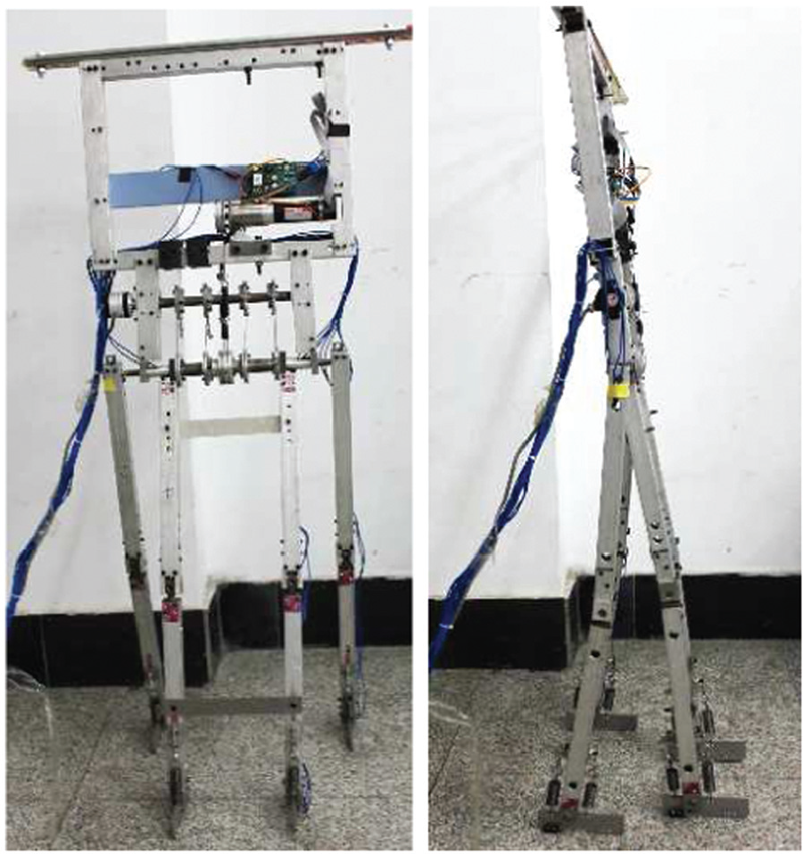
Physical prototype.

The mechanical cost of transport defined in equation (19) was calculated by the data collected from sensors at the DC motor and hip joint each step to analyze the energy consumption of our the prototype during walking, where L is the step length

c_{mt} = \frac{(\sum_{i = 1}^{n} \int_{0}^{T} | τ . {\overset{\cdot}{ϕ}}_{i} | \cdot dt)}{mg \cdot L}

(20)

Figure 12 shows the effect of K_p on the mechanical cost of transport. Both the simulation and experimental results show that the mechanical cost of transport increases with the increasing value of K_p . The reason is that the increase in K_p injects higher torque value to the hip joint which costs more energy.

Figure 12.

Effect of K_p on mechanical cost of transport.

Figure 13 shows the frames from the experiments’ video of one successful walking experiment. The passive robot could walk on level ground stably with certain walking speed by giving a proper initial value manually.

Figure 13.

Frames from experiments’ video.

Conclusion

In this article, a detailed design process of the mechanical structures and control system architecture for a passive dynamic biped walking robot is introduced. A detailed walking dynamics for the passive model that consisted of an upper body, two legs, two flat feet, a hip joint, two knee joints, and two ankle joints is derived based on virtual power principle. The instant just before foot-ground impact is chosen as the start point of the walking, which can reduce the number of independent state variables and thus increase the chance of finding out the fixed point. The walking exhibits a more natural gait that contains a double stance phase. We prove the correctness of the walking dynamics by the numerical simulation process in MATLAB. Finally, we built a physical prototype based on the design and the experimental results prove that the design of the passive dynamic walking robot is rational in this study.

As described in this study, the passive dynamic walking robot can walk successfully both on a shallow slope without any control and on level ground with only simple PD control at the hip joint. However, to obtain a better walking performance and more versatile walking gait, the ankle joint control must be induced. So the future work will focus on the study of ankle joint actuation.

Footnotes

Acknowledgements

Thanks are due to Yanhe Zhu, Xizhe Zang, and Jie Zhao for their help and valuable advices.

Academic Editor: Yong Chen

Declaration of conflicting interests

The author(s) declared no potential conflicts of interest with respect to the research, authorship, and/or publication of this article.

Funding

The author(s) disclosed receipt of the following financial support for the research, authorship, and/or publication of this article: This research was funded and supported by “the Fundamental Research Funds for the Central Universities” (grant no. HIT.NSRIF.2012039) and “Independent Research of State Key Laboratory of Robotics and System (HIT)” (grant no. SKLRS201304B).

References

Sakagami

Watanabe

Aoyama

. The intelligent Asimo: system overview and integration. In: IEEE/RSJ international conference on intelligent robots and systems, Lausanne, 30 September–4 October 2002, pp.2478–2483. New York: IEEE.

Kaneko

Kanehiro

Kajita

. Humanoid robot HRP-2. In: Proceedings of the IEEE international conference on robotics and automation, New Orleans, LA, 26 April–1 May 2004, pp.1083–1090. New York: IEEE.

Collins

Ruina

. A bipedal walking robot with efficient and human-like gait. In: Proceedings of the 2005 IEEE international conference on robotics and automation (ICRA 2005), Barcelona, 18–22 April 2005, pp.1983–1988. New York: IEEE.

McGeer

. Passive dynamic walking. Int J Robot Res 1990; 9: 62–82.

McGeer

. Passive walking with knees. In: Proceedings of the IEEE conference on robotics and automation, Cincinnati, OH, 13–18 May 1990, pp.1640–1645. New York: IEEE.

Collins

Wisse

Ruina

. A three-dimensional passive-dynamic walking robot with two legs and knees. Int J Robot Res 2001; 20: 607–615.

Hobbelen

DGE

Wisse

. Chapter 14. Limit cycle walking. In: Hackel

(ed.) Humanoid robots, human-like machines. Vienna: ITech Education and Publishing, 2007, pp.277–294.

Wisse

Schwab

Van der Linde

. How to keep from falling forward: elementary swing leg action for passive dynamic walkers. IEEE T Robot 2005; 21: 393–401.

Bhounsule

Cortell

Grewal

. Low-bandwidth reflex-based control for lower power walking: 65 km on a single battery charge. Int J Robot Res 2014; 33: 1305–1321.

10.

Hobbelen

DGE

Wisse

. Ankle actuation for limit cycle walkers. Int J Robot Res 2008; 27: 709–735.

11.

Ruina

Bertram

JEA

Srinivasan

. A collisional model of the energetic cost of support work qualitatively explains leg sequencing in walking and galloping, pseudo-elastic leg behavior in running and the walk-to-run transition. J Theor Biol 2005; 237: 170–192.

12.

Wisse

Hobbelen

DGE

. Ankle springs instead of arc-shaped feet for passive dynamic walkers. In: IEEE-RAS international conference on humanoid robots, Genova, 4–6 December 2006. New York: IEEE.

13.

Huang

Wang

Gao

. Modeling and analysis of passive dynamic bipedal walking with segmented feet and compliant joints. Acta Mech Sinica 2012; 28: 1457–1465.

14.

Pratt

Williamson

. Series elastic actuators. In: “Human robot interaction and cooperative robots.” Proceedings of the IEEE/RSJ international conference on intelligent robots and systems 95, Pittsburgh, PA, 5–9 August 1995, vol. 1. New York: IEEE.

15.

Schwab

Wisse

. Basin of attraction of the simplest walking model. In: Proceedings of the ASME design engineering technical conference, Pittsburgh, PA, 9–12 September 2001, vol. 6. New York: ASME.

16.

Wisse

Hobbelen

DGE

Schwab

. Adding the upper body to passive dynamic walking robots by means of a bisecting hip mechanism. IEEE T Robot 2007; 23: 112–123.

17.

Hobbelen

De Boer

Wisse

. System overview of bipedal robots flame and tulip: tailor-made for limit cycle walking. In: IEEE/RSJ international conference on intelligent robots and systems (IROS 2008), Nice, 22–26 September 2008. New York: IEEE.

18.

Goswami

Thuilot

Espiau

. Compass-like biped robot—part I: stability and bifurcation of passive gaits. INRIA Research Report no. 2996, October 1996. Le Chesnay: INRIA.

19.

Spong

Hutchinson

Vidyasagar

. Robot modeling and control. Hoboken, NJ: John Wiley & Sons, 2006.

20.

Duindam

. Port-based modeling and control for efficient bipedal walking robots, 2006, http://eprints.eemcs.utwente.nl/1622/01/vduindamPhDthesis.pdf

21.

Hsu

. Global analysis by cell mapping. Int J Bifurcat Chaos 1992; 2: 727–771.

System overview and walking dynamics of a passive dynamic walking robot with flat feet

Abstract

Keywords

Introduction

Mechanical structure design process

Overall design

Upper body and SEA design

Knee joint design

Ankle joint design

Control system architecture

Walking phases and walking dynamics

Walking phases

Phase a: first foot-ground impact

Phase b: first double stance

Phase c: second foot-ground impact

Phase d: second double stance

Phase e: four-link swing phase

Phase f: knee impact

Phase g: three-link swing phase

Walking dynamics

Numerical simulation and experiments

Numerical simulation

Experiments

Conclusion

Footnotes

Acknowledgements

Declaration of conflicting interests

Funding

References