Sage Journals: Discover world-class research

Abstract

In this paper, we propose a locomotion control method for a compliant legged robot from slow walking to fast running. We also examine the energy efficiency of the compliant legged robot controlled by the proposed locomotion control method. Experimentally, we obtain the robot running speed of about 4.3m/s with the initial compliant leg length of 0.1m. In addition, we obtain very good energy efficiency. In the best case, the mechanical cost of transport(Cmt), known as an energy efficiency measure, is obtained at about 0.2. Comparing with the other energy efficient robots, our robot exhibits very good energy efficiency.

Keywords

Compliant Legged Robot Spring-Mass Model Self-Stability Cost of Transport Mechanical Cost of Transport

1. Introduction

“How do animals move?”[1] – animals' movement is the exchange of energy storage and recovery[1]. Animal walking is generally modelled as an inverted pendulum[1] and animal running is generally modelled as the spring-mass system[1]. However, Geyer et al.[2] show that the walking is more properly explained as modelled by the spring-mass system used for running. We propose to develop an energy efficient robot mimicking the animal movement, such as the exchange of energy storage and recovery, and the leg structure is made as a compliant leg along the lines of a spring-mass system.

Our proposed locomotion control method is fundamentally as follows. Firstly, the locomotion control method generates the robot leg touch down angle with regard to the locomotion speed within the self-stable region[2,3]. Secondly, the touched robot leg angle trajectory is generated by using the spring-mass model. The above two methods lead to robot energy efficiently, because the above two methods need no energy consumption for robot locomotion and locomotion stability in cases of the constant speed and energy lossless. That is, the above two methods need energy consumption for acceleration, deceleration and energy losses. Finally, the locomotion control method uses different time intervals between the feedback control loop sampling time and the trajectory generation time. This allows the slow walking and fast running of the robot. The detailed explanation is described in chapter 2.

In previous related works, McGeer's passive dynamic walker[4] is powered only by gravity, without active control or energy input. However, it can only walk down a slope, i.e., it cannot walk on level ground[5]. Collins et al.[5] developed several robots based on the above passive dynamic walker, with a small active power source, which can walk on level ground using simple control and little energy. But these robots can walk at only a specific walking speed[6]. Sreenath et al.[7] developed the planar bipedal robot MABEL for stable, energy efficient and fast bipedal walking. MABEL obtained a very good energy efficiency, the best case is Cmt≈0.14(Cmt will be explained in chapter 3), and obtained a walking speed of 1.5m/s with robot leg length 1m. In addition, MABEL obtained a running speed of 3m/s[8]. The ARL monopod II[9], which is based on the Controlled Passive Dynamic Running(CPDR) strategy, obtained a running speed of up to 1.25m/s and Cmt≈0.22. The other control methods for legged robots are based on the Central Pattern Generator(CPG)[10], Genetic Algorithm(GA)[11] and neuro-fuzzy learning algorithm[12].

The locomotion control method proposed in this paper provides stable, energy efficient locomotion from slow walking to fast running and this method is simple, easily applicable and practical.

This paper is organized as follows. In chapter 2, we explain the proposed locomotion control method. In chapter 3, we examine experimentally the results of the proposed locomotion control method. Finally, in chapter 4, we summarize and conclude this paper.

2. Locomotion Control Method

Our compliant legged robot can be modelled simply as shown in Figure 1. In Figure 1, m is the point mass representing the compliant legged robot mass. x and y are the position coordinates of the point mass m, K is the stiffness coefficient of the compliant leg, l0 is the initial compliant leg length, l1 and l2 are the compressed compliant leg lengths, τ₁ and τ₂ are the control input torques, F₁ and F₂ are the compressed compliant leg forces(F_i=K(l₀-l_i), i=1,2), θ₁ and θ₂ are the leg angles relative to the vertical line (the positive leg angle is defined clockwise and the negative leg angle is defined counter clockwise), x_g1, y_g1, x_g2 and y_g2 are the leg touch positions on the ground, where the subscript 1 means leg 1 and the subscript 2 means leg 2. In Figure 1(b), there is no subscript, this means any one of leg 1 or 2. That is, in running case, any one of leg 1 or 2 touch on the ground, and next the other leg touch on the ground. In Figure 1(c), α₀ is the leg touch down angle on the ground, α is the varied leg angle on the ground, y_apex,p(p=i,i+1,i+j,i+j+1) are the apex heights at the p^th apex, V_x,apex,p(p=i,i+1,i+j,i+j+1) are the velocities of the x direction at the p^th apex, g is the gravitational acceleration(g=9.81m/s2). In this paper, we assume the robot leg is massless and we use the symbols in Figure 1 in common.

Figure 1.

(a) Walking-double leg support spring-mass model, (b) running-single leg support spring-mass model, (c) walking/running model

The dynamics of Figure 1 is derived from the free body diagram for the point mass m as follows:

\begin{array}{l} m \overset{..}{x} = F_{1} \sin θ_{1} + F_{2} \sin θ_{2} + τ_{1} \frac{\cos θ_{1}}{l_{1}} + τ_{2} \frac{\cos θ_{2}}{l_{2}} \\ m \overset{..}{y} = F_{1} \cos θ_{1} + F_{2} \cos θ_{2} - m g + τ_{1} \frac{- \sin θ_{1}}{l_{1}} + τ_{2} \frac{- \sin θ_{2}}{l_{2}} \end{array}

(1)

The proposed locomotion control method is as shown in Figure 2.

Figure 2.

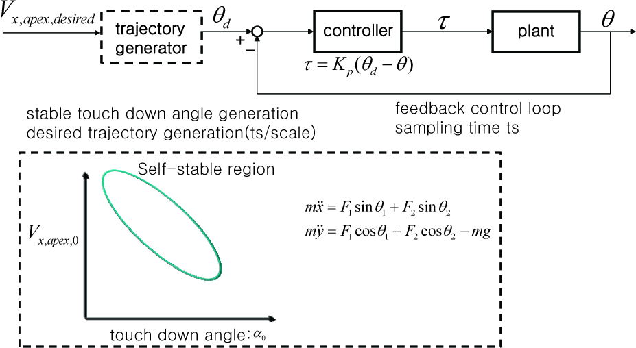
Locomotion control method

In Figure 2, the plant is the compliant legged robot and the controller performs simple P (Proportional) control for the robot leg angles. In addition, in Figure 2, the trajectory generator receives V_{x,apex,desired}(the desired velocity of x direction at apex) and generates a stable touch down angle α₀ with regard to V_{x,apex,desired} (V_x,apex,0 (the velocity of x direction at initial apex) in the self-stable region in Figure 2.), generating the robot leg touch down angle θ₀ = –(90⁰ – α₀). The trajectory generator generates the desired robot leg angle trajectory for the untouched leg on the ground from apex to touch down (Equation (2)) and from take-off to apex (Equation (3)) in walking and running in Figure 1(c) as follows:

θ_{i d} = \frac{(θ_{0} - θ_{a p e x})}{T_{s w}} (t - t_{a p e x}) + θ_{a p e x} (i = 1, 2)

(2)

θ_{i d} = \frac{(θ_{a p e x} - θ_{T O})}{T_{s w}} (t - t_{T O}) + θ_{T O} (i = 1, 2)

(3)

where θ_id(i = 1,2) is the desired robot leg angle, t_apex is time at apex, t_TO is time at take-off, t is time of the robot locomotion, θ_apex is the robot leg angle at apex which we define -π / 3, θ_TO is the robot leg angle at take-off and T_sw is the robot leg swing time from apex to touch down (Equation (2)) and from take-off to apex (Equation (3)) which we obtain with tuning with regard to scale value (explained later in this chapter).

The trajectory generator generates the desired robot leg angle trajectory for the touched leg on the ground from the unforced natural dynamics of the compliant legged robot, that is, τ₁,τ₂ = 0 in Equation (1). This unforced natural dynamics is used for the analysis of self-stability [2,3]. Solving the unforced natural dynamics using the numerical integration method (we used the 4^th order Runge-Kutta method) we obtain the desired trajectory of the robot x_d and y_d, and obtain the desired robot leg angle trajectory as follows:

θ_{i d} = \tan^{- 1} (\frac{x_{d} - x_{g i}}{y_{d} - y_{g i}}), (i = 1, 2)

(4)

where θ_id(i = 1,2) is the desired robot leg angle, x_gi(i=1,2) is determined by x_i = x_d − l₀ sin θ₀(i = 1,2) at touch down of the i^th leg, y_gi(i=1,2) is assigned to 0 because we assume the level ground. So we obtain one desired robot leg angle for the touched leg θ_id (i = 1 or 2) in the single leg phase of walking and in the stance phase of running in Figure 1(c), and obtain two desired robot leg angles for the touched legs θ_id (i = 1 and 2) in the double leg phase of walking in Figure 1(c).

Therefore, the trajectory generator generates the desired robot leg angle trajectory for the touched and the untouched leg on the ground.

For the slow walking and the fast running, we change the desired trajectory generation time of the robot from the feedback control loop sampling time ts, using ts=0.001sec.

For the slow walking, we adjust the scale value of ts/scale in Figure 2 to greater than 1, this makes the desired trajectory generation time of the robot shorter than ts, so the numerical integration time is shorter than ts. The result is a shorter desired trajectory interval of the robot and a shorter desired robot leg angle trajectory interval for the touched leg on the ground than that of ts, that is, scale value 1. In Equations (2) and (3), T_sw is tuned with regard to scale value by T_sw=0.03sec x scale, so the scale value is greater than 1, T_sw is longer than 0.03sec in the case of scale value 1. The result is a shorter desired robot leg angle trajectory interval for the untouched leg on the ground than that of scale value 1. These make the robot move slowly.

Oppositely, for the fast running, we adjust the scale value to smaller than 1, making the desired trajectory generation time of the robot longer than ts, so the numerical integration time is longer than ts. The result is a longer desired trajectory interval of the robot and a longer desired robot leg angle trajectory interval for the touched leg on the ground than that of ts, that is, scale value 1. In addition, in Equations (2) and (3), the scale value is smaller than 1, T_sw is shorter than 0.03sec in the case of scale value 1. The result is a longer desired robot leg angle trajectory interval for the untouched leg on the ground than that of scale value 1. These make the robot move faster.

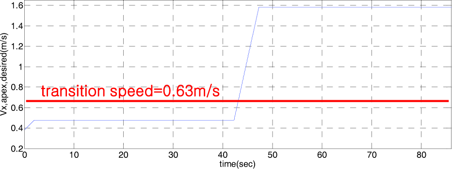
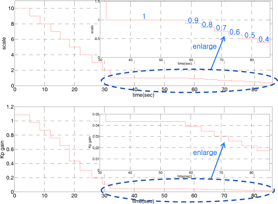
According to scale value, we tune the P (Proportional) gain Kp in Figure 2 as shown in Figure 7 because, in slow motion, the required leg support torque is too large, so the Kp is tuned to high. In fast motion, due to the limitation of the actuator power, Kp is tuned to low.

Figure 3.

The experimental compliant legged robot and the experimental condition

Figure 4.

The compliant leg of the experimental robot

Figure 5.

The self-stable regions of the walking and running

Figure 6.

V_{x,apex,desired}

Figure 7.

Scale and Kp gain

Predicting the energy efficiency, the energy efficiency of the cases where scale value is greater and smaller than 1 is expected to lower than that of the case where scale value is 1. This is because, in cases where scale value is greater and smaller than 1, this intentionally makes the robot move slow and fast, so this movement is unnatural, but where scale value is 1, this makes the robot move naturally. The energy efficiency results are discussed in chapter 3.

3. Experiment

In this chapter, we experiment with the compliant legged robot controlled by the locomotion control method explained in chapter 2. From this we can examine the length of time that the robot walks slowly and runs quickly, and if the robot moves energy efficiently.

The experimental compliant legged robot and the experimental condition are shown in Figure 3.

As shown in Figure 3, the experimental condition is the constraint locomotion. The compliant leg of the experimental robot is shown in Figure 4.

The leg spring is indicated by the circle in Figure 4. The leg has three springs with phase 120⁰. The reason why we used this structure is that the robot leg rotates one directionally for walking and running. If we want the robot leg to rotate bidirectionally for walking and running, we need to use another actuator for bending the robot leg or adjusting the robot leg length because the bidirectional rotating robot leg touches the ground. We intended to use as few as possible actuators for the robot. We use two motors for the left and right leg of the experimental robot. The motor is a maxon EC-4pole 30(200W, 24V, nominal speed: 16200rpm, nominal torque: 114mNm)[13] and the reduction gear is a maxon Planetary Gearhead GP 32 HP 33:1[13].

The parameters of the experimental robot are as shown in Table 1.

Table 1.

The parameters of the experimental robot

	design value	manufactured value
mass m(kg)	3	3.45
stiffness K(N/m)	11772	12070
dimensionless reference stiffness[3]	40	35.66
initial leg length l₀(m)	0.1	0.1

The self-stable regions of the walking and running are shown in Figure 5 based on the design parameter values of the experimental robot.

In Figure 5, ‘*’ denotes the minimum stable touch down angle with regard to each related V_x,apex,0, ‘x’ denotes the maximum stable touch down angle and ‘+’ denotes the mean stable touch down angle. The dotted line and the solid line in the self-stable region of the walking is the mean value fitting line and the mean value-2 degree fitting line, respectively. In addition, the solid line in the self-stable region of the running is the mean value fitting line.

The self-stable regions in Figure 5 are obtained based on the design parameter-dimensionless reference stiffness 40. In the case of the manufactured parameter-dimensionless reference stiffness 35.66, which is a little smaller than 40, the self-stable regions are moved a little to the left and down. This tendency can also be seen in Figure 5 of the reference [3].

In the experiment, we use the stable touch down angle of the walking and running on the solid lines in Figure 5 with regard to V_{x,apex,desired}. This is obtained because the manufactured parameter-dimensionless reference stiffness 35.66 is a little smaller than the design parameter-dimensionless reference stiffness 40 and by a little tuning.

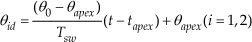
In the experiment, we use V_{x,apex,desired} as in Figure 6. As the V_{x,apex,desired} in Figure 6, we give the walking speed, from walking to running transition speed, acceleration and the running speed as the desired speed at apex. Here, we set the transition speed to 0.63m / s based on the V_{x,apex,desired}. The reason why we set the transition speed to 0.63m/s is as follows: the transition speed of the human being is known to be about 2m/s in the case where the human's leg length is 1m[3]. From this, using the Froude number [14], we obtain Fr = v² / gl₀ = 2² / (9.81 × 1), and with the initial compliant leg length of the experimental robot l₀=0.1m, we obtain $v = \sqrt{F r \times g \times 0.1} = 0.63 m / s$ .

As explained in chapter 2, the trajectory generator receives V_{x,apex,desired} in Figure 6 and generates the stable touch down angle of the walking and running on the solid lines in Figure 5 with regard to V_{x,apex,desired}. This then generates the desired robot leg angle trajectory for the untouched leg on the ground using Equations (2) and (3), and also generates the desired robot leg angle trajectory for the touched leg on the ground using Equation (1) with τ₁,τ₂ = 0 and the manufactured parameters m, K, l₀ in Table 1 and Equation (4).

In the experiment, the scale value and the Kp gain explained in chapter 2 are used as in Figure 7.

The results of the above locomotion control method applying the experimental compliant legged robot are as shown in Figure 8.

Figure 8.

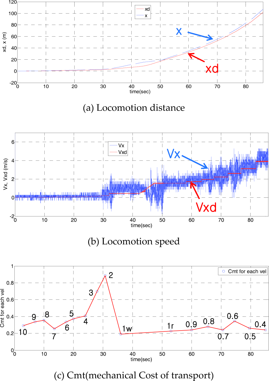
The experimental results

The desired(xd) and the real(x) locomotion distance are as shown in Figure 8(a) and the desired(Vxd) and the real(Vx) locomotion speed are as shown in Figure 8(b). The xd and Vxd are obtained by numerical integration (here we use the 4^th order Runge-Kutta method) of Equation (1) with τ₁,τ₂ = 0, the manufactured parameters m, K, l0 in Table 1, using the scale value in Figure 7. In addition, the x and Vx are obtained by x=R θ_x and Vx=R ${\dot{θ}}_{x}$ , R is the constraint bar length in Figure 3 which is from the centre of the robot rotation axis to the robot mass centre, this is R=1.5m, θ_x is the angle of the robot rotation which is measured by the X axis encoder in Figure 3, and ${\dot{θ}}_{x}$ is the angular velocity of the robot rotation which is obtained by the differentiation of θ_x. In Figure 8(b), Vx value is fluctuating, this is mainly due to the flexible constraint bar in Figure 3 which vibrates when the robot touches down on the ground while walking and running. In Figure 8(b), from about 33sec to about 43sec, this contains the region of walking with scale value 1, the mean of Vx is higher than Vxd. This is also observable from Figure 8(a) - the slope of x is greater than that of xd. Additionally, in Figure 8(b), from about 43sec to 50sec, this contains acceleration, transition from walking to running and the front region of running with scale value 1 - Vx is lower than Vxd. This is also observable from Figure 8(a) - the slope of x is smaller than that of xd. In the other regions of Figure 8(b), the mean of Vx is similar to Vxd, but not closely similar because we do not use feedback control for Vx, we only use open-loop control. In the other regions of Figure 8(a), the slope of x is similar to that of xd.

From Figure 8(b), the minimum real mean walking speed is obtained as about 0.068m/s with the initial compliant leg length 0.1m at the scale value 10. This is slow walking. Of course, the robot can maintain stance at the stopped state and the maximum real mean running speed is obtained as about 4.3m/s with the initial compliant leg length 0.1m at the scale value 0.4. This is extremely fast running. These results were obtained as explained in chapter 2.

Next, we examine the energy efficiency of the compliant legged robot controlled by the above locomotion control method. We use Cmt(mechanical Cost of transport)[5] as the energy efficiency measure which is generally used as the energy efficiency measure. Cmt is defined as Cmt=P/MgV, P is the mechanical output power of the actuators, M is the mass of the robot, g is the gravitational acceleration and V is the speed of the robot. As for the definition of the Cmt, Cmt is a dimensionless value - the smaller Cmt, the higher the energy efficiency. Here, we use the mean value of P and V, g is 9.81m/s², and M is 5kg because the manufactured robot mass is 3.45kg and the additional mass due to the constraint bar and the wire in Figure 3 is 1.55kg. The experimental results of the Cmt are as shown in Figure 8(c). In Figure 8(c), 10,9,…,0.4, the numbers on the figures are the scale values. The 1w is scale value 1 in walking and the 1r is scale value 1 in running. Of course, the scale values from 10 to 2 are walking because these cases are below the transition speed and the scale values from 0.9 to 0.4 are running because these cases are above the transition speed.

As we predicted in chapter 2, the Cmt values of the cases of which the scale value is 1 are smaller than those where the scale values are greater and smaller than 1. That is, the energy efficiency where the scale value is 1 is higher than that where the scale values are greater and smaller than 1. Similar results were obtained several times from equivalent experiments.

In Figure 8(c), the minimum value of Cmt is about 0.2. The Cmt values of the previously well known and energy efficient robots are as follows. The Cmt of Honda's Asimo is 1.6[5]. The Cmt of the Cornell biped is 0.055[5], this robot is highly energy efficient but it can only walk at one preferred speed[6]. The Cmt of the Rabbit is 0.38[7]. The minimum Cmt of the MABEL is 0.14[7]. The Cmt of the ARL monopod II is 0.22[9], and the Cmt of the Scout II is 0.47[15]. Compared with the above robots, the energy efficiency of our compliant legged robot controlled by the above locomotion control method is not the best, but very good. In future works, we plan to improve the energy efficiency of our robot by optimizing the mechanism of our robot and the control method.

In this chapter, we obtained experimentally slow walking to fast running and a very good energy efficiency with the proposed locomotion control method for the compliant legged robot.

4. Conclusion

In this paper, we proposed the locomotion control method for the compliant legged robot from slow walking to fast running. In addition, we examined the energy efficiency of the compliant legged robot controlled by the proposed locomotion control method.

We obtained the minimum real mean walking speed 0.068m/s with the initial compliant leg length 0.1m including stance at the stopped state. We also obtained the maximum real mean running speed 4.3m/s with the initial compliant leg length 0.1m. That is, the robot moves 43 times longer than with the initial compliant leg length per second. This is extremely fast running.

The energy efficiency where the scale value is 1 is higher than that where the scale values are greater and smaller than 1. This result is obtained experimentally as we predicted in chapter 2.

In the best case, we obtained the Cmt 0.2. This result is a very good energy efficiency compared to the other energy efficient robots.

The locomotion control method proposed in this paper provides stable, energy efficient locomotion from slow walking to fast running and this method is simple, easily applicable and practical.

Footnotes

5. Acknowledgments

This work was supported by the DGIST R&D Programme of the Ministry of Education, Science and Technology of Korea(12-BD-0101).

References

Dickinson

M. H.

Farley

C. T.

Full

R. J.

Koehl

M. A. R.

Kram

and Lehman

(2000) How Animals Move: An Integrative View. Science, vol. 288, no. 5463, pp. 100–106.

Geyer

Seyfarth

Blickhan

(2006) Compliant leg behaviour explains basic dynamics of walking and running. Proc. R. Soc. B, 273, pp. 2861–2867.

Rummel

and Seyfarth

(2008) Stable Running with Segmented Legs. The International Journal of Robotics Research, vol. 27, no.8, pp. 919–934.

McGeer

(1990) Passive Dynamic Walking. The International Journal of Robotics Research, vol. 9, no. 2, pp. 62–82.

Collins

Ruina

Tedrake

Wisse

(2005) Efficient Bipedal Robots Based on Passive-Dynamic Walkers. Science, vol. 307, no. 5712, pp. 1082–1085.

Seyfarth

Iida

Tausch

Stelzer

von Stryk

and Karguth

(2009) Towards Bipedal Jogging as a Natural Result of Optimizing Walking Speed for Passively Compliant Three-Segmented Legs. The International Journal of Robotics Research, vol. 28, no. 2, pp. 257–265.

Sreenath

Park

H. W.

Poulakakis

, and Grizzle

J. W.

(2011) A Compliant Hybrid Zero Dynamics Controller for Stable, Efficient and Fast Bipedal Walking on MABEL. The International Journal of Robotics Research, vol. 30, no. 9, pp. 1170–1193.

http://www.youtube.com/watch?v=xlOwk6_xpWo

Ahmadi

and Buehler

(1999) The ARL Monopod II Running Robot: Control and Energetics. IEEE International Conference on Robotics & Automation, pp. 1689–1694.

10.

Rutishauser

Spröwitz

Righetti

and Ijspeert

A. J.

(2008) Passive compliant quadruped robot using central pattern generators for locomotion control. Proceedings of the 2nd Biennial IEEE/RAS-EMBS International Conference on Biomedical Robotics and Biomechatronics, pp. 710–715.

11.

Cardenas-Maciel

S. L.

Castillo

and Aguilar

L. T.

(2011) Generation of walking periodic motions for a biped robot via genetic algorithms. Applied Soft Computing, vol. 11, no. 8, pp. 5306–5314.

12.

Cardenas-Maciel

S. L.

Castillo

and Aguilar

L. T.

(2011) Neuro-Fuzzy Based Output Feedback Controller Design for Biped Robot Walking. Soft Computing for Intelligent Control and Mobile Robotics, pp. 423–444.

13.

maxon motor catalog 2010/11

14.

Rummel

Iida

Smith

J. A.

and Seyfarth

(2008) Enlarging Regions of Stable Running with Segmented Legs. IEEE International Conference on Robotics and Automation, pp. 367–372.

15.

Poulakakis

Smith

J. A.

and Buehler

(2005) Modeling and Experiments of Untethered Quadrupedal Running with a Bounding Gait: The Scout II Robot. The International Journal of Robotics Research, vol. 24, no. 4, pp. 239–256.

Locomotion Control of a Compliant Legged Robot from Slow Walking to Fast Running

Abstract

Keywords

1. Introduction

2. Locomotion Control Method

3. Experiment

4. Conclusion

Footnotes

5. Acknowledgments

References