
Abstract
Humanoid biped robots are typically complex in design, having numerous Degrees-of-Freedom (DOF) due to the ambitious goal of mimicking the human gait. The paper proposes a new architecture for a biped robot with seven DOF per each leg and one DOF corresponding to the toe joint. Furthermore, this work presents close equations for the forward and inverse kinematics by dividing the walking gait into the Sagittal and Frontal planes. This paper explains the mathematical model of the dynamics equations for the legs into the Sagittal and Frontal planes by further applying the principle of Lagrangian dynamics. Finally, a control approach using a PD control law with gravity compensation was recurred in order to control the desired trajectories and finding the required torque by the joints. The paper contains several simulations and numerical examples to prove the analytical results, using SimMechanics of MATLAB toolbox and SolidWorks to verify the analytical results.
1. Introduction
In recent years, several efforts of the robotics community have focused on developing bio-inspired robots, particularly in humanoid biped robots. This has resulted in promising developments such as the ASIMO (the acronym of “Advanced Step In Mobility”) humanoid robot, developed by Honda with 32 DOF and 52 kg weight [1] or the 62-kg MAHRU series of Samsung Electronics with 32 DOF [2]. Further examples of contributions in the humanoid robots field are the QRIO, which has an adaptable motion controller that allows the displacement on uneven surfaces and external forces [3] and the WABIAN series of Waseda University with 35 DOF [4], which has played a fundamental role in the evolution of humanoid robots. Some of the most studied architectures found in the literature include the H7 from the University of Tokyo with a total of 30 DOF, seven for each leg including a one DOF toe joint, seven DOF for each arm, including a single DOF gripper and two DOF at the neck [5]. Another example is the JOHNNIE robot from the Technical University of Munich, where each leg incorporates six driven joints, three DOF in the hip, one DOF for the knee, and another two DOF for the ankle joint [6]. Nowadays, most of the humanoid robots mentioned above consist of two 6-DOF legs, namely 3-DOF hip, 1-DOF knee and 2-DOF ankle. Although the efforts have mainly focused on achieving human gait, this feature has not been successful accomplished with a limited number of DOF. Thus, it becomes necessary to incorporate redundant DOF in order to achieve an approximate human gait motion [7].
The addition of an active toe joint to the kinematic model of each leg has drawn enormous interest within the robotics scholars, because compared with conventional humanoid robots that are equipped with flat feet, this architecture allows a robot to walk in a more natural way. There are several references in the literature related to toe joints in biped robots. For example, Kumagai et al. developed a biped robot which has 7 DOF at each leg including a passive toe joint [8]. Kumazawa et al. [9] and Ogura et al. [10] proposed an elastic toe joint mechanism; the passive joint, which was selected by analysing human gait analysis reports. The toe joint was then developed as a hinge joint. However, in order to improve the toe functionality, an active joint control is required for keeping a multipoint contact with the floor. Konno et al. [11] included passive toe joints with torsion springs in order to achieve human-like gait based on biomechanical studies. Scarfogliero et al. [12] equipped the passive toe joints with spring-damper buffers for a smoother foot rotation. Koganezawa et al. [13] proposed a hybrid active/passive design for lower energy consumption during walking. Nishiwaki et al. [14] added an active toe joint to each 6 DOF leg to achieve high walking speed, high step climbing, and knee down motion with the sole attached to the ground. Furthermore, the authors used toe joint rotation during the double support phase to decrease the knee joint angular velocity, resulting in a 1.8 times faster gait motion due to the active toe joints. Nevertheless, using the toe joint only in the double support phase, strongly limits the advantages introduced by this feature. In fact, during the double support phase it is also possible to introduce a foot rotation about the front edge, which leads to similar results. Finally, the gait results in an unnatural motion due to the fact that the humanoid cannot stretch the knees. Sellaouti et al. [15] focused on walking speed augmentation in a 6 DOF leg through the use of passive toe joints during the single support phase, achieving a 1.5 times faster gait motion. This result is due to the integration of an under actuated phase at the end of the single support phase, where the support foot rotates around the toe joint and allows the ankle joint to rise. It was also noticed that when passing the straight leg singularity, the robot was able to fulfil larger steps and increase its walking speed. This robot however, has an unnatural gait, since the humanoid has to lower its centre of mass closer to the ground in order to get large steps. Kumar et al. [16] presented a 2 DOF leg with a passive toed feet that can walk down a gentle slope under the action of gravity alone using ankle-strike as a mean to progress to toe-rotation phase. The lack of an active joint prevents this architecture to walk on any other surface than a downward slope. From the abovementioned robotic architectures, the development of a robotic leg with more than 6 DOF and an active toe joint that would enable walking in a more natural manner has yet to be proposed.
This paper suggests a new architecture for a biped robot with seven DOF per leg, adding one DOF that imitates the toe joint. In this kinematic chain all the joints are active, in contrast to the previously mentioned architectures, which have six or seven DOF without a toe joint or with a passive toe joint. The authors believe that with this new architecture, the humanoid robot will be able to walk with the knee stretched. This is due to the fact that the walking patterns of many biped robots are calculated by solving six dimensional inverse kinematics based on the position and orientation of the foot and the waist, meaning that the seven DOF leg would provide the necessary redundancy to avoid the singularity problem presented in humanoids. This paper presents a comprehensive study of the forward and inverse kinematics of the new architecture for a humanoid leg.
The modelling of biped gait has usually resulted in the description of kinematics, dynamics and stability of two-legged walking robots and represents an unresolved challenge, as most approaches reduce the dynamic model of the humanoid robot to an inverted pendulum that is based upon either a simple observation or mathematical analysis, derived from kinematics [17]. A different approach suggests that walking motion, with static balance, could be achieved by solving simple kinematics equations. However, the static approach results in undesirable constraints on both the biped structure and walking efficiency [18]. Although these methods are valid for studying the walking stability of a humanoid robot, they do not solve complex stability problems such as modelling the human gait motion [19]. An alternative way to derive mathematical dynamics and achieve a stable biped locomotion is the use of Lagrangian dynamics. This technique has been especially successful in providing an understanding of the unstable dynamics associated with biped posture and enables the design of effective stabilization controls for robots [20]. The Lagrange-Euler formulation has been used in [21] to solve the problem of dynamically balanced gait generation by determining the joint torques for a 7 DOF two-legged robot. The Lagrangian equation has been used in [22] to obtain the dynamic model for of a five link biped where each leg has 2 DOF, applying a conventional Proportional- Derivative (PD) controller in which the locomotion is constrained within the Sagittal plane to control the stability of a human gait. Further studies approach the dynamics by restricting the motion for the Sagittal plane for a five link biped robot [23] and a nine-link biped robot model with 3 DOF in each leg [24]. This paper uses the Lagrangian dynamic model for finding the close-form equations that model dynamic behaviour by means of dividing the legs into the Sagittal and Frontal planes, which simplify the mathematical model and further applies PD control law with gravity compensation to determine the desired position and torque for each joint.
This paper is organized as follows. In Section 2, the forward kinematics for the proposed humanoid robot is obtained using the Denavit-Hartenberg convention. This is followed by Section 3, which presents the inverse kinematics in the Sagittal and Frontal planes. Section 4 includes trajectory planning for controlling the biped robot through periodic motion in order to produce a stable gait. The discussion about the dynamic model in the Sagittal and Frontal planes using Lagrange equations is in Section 5. Several simulation results using MATLAB SimMechanic are compared with numerical examples, which demonstrate the plausibility of the analytical equations in Section 6. Finally, Section 7 presents some important conclusions and suggestions for future research on this new architecture for a humanoid biped robot.
2. Forward Kinematics
In robotics literature, forward kinematics is commonly known as the task in which the position and orientation of the end-effector is to be determined by giving the configurations for the active joints of the robot [23]. This paper focuses on the lower body of a humanoid biped robot as shown in Figure 1. It consists of two 8 DOF legs, namely a 3 DOF hip, a 1 DOF knee, a 3 DOF ankle and 1 DOF that imitates the toe joint. Each leg can be modelled as a kinematic chain with nine links connected by eight revolute joints.

Kinematic description of the robot leg
The synthesis of the kinematic chains is based on human body parameters in terms of ratios, range of motion, and physical length [24]. Table 1 shows the range of motion for the human leg, while the parameters corresponding to the robot leg are based on a previous study by Hernandez-Santos et al [25]. Note that some ranges of motion of the humanoid robot do not correspond to the human leg, due to the interference between mechanical parts.
Joint range of motion

The local frames (Xi, Yi, Zi) are assigned to each joint according to the Denavit-Hartenberg (DH) convention [26]. Consider the base frame (X0, Y0, Z0) at the centre of the waist as the global reference frame. Since the general kinematic structures of the left leg of a humanoid robot are identical to those of the right leg, this paper assigns the same coordinate frames for the left and right limbs for convenience of analysis. Figure 1 shows the designated local coordinate frames for the right leg, where li denotes the length of link i. Table 2 shows the DH parameters where θi is the angle between the Xi-1 and Xi axes as measured about the Zi-1 axis; di is the distance from the Xi-1 to the Xi axis as measured along the Zi axis; ai is the distance from the Zi-1 to Zi axis measured along the Xi-1 axis; and αi is the angle between the Zi-1 and Zi axes measured about the Xi-1 axis. The angles are assumed positive, counterclockwise about the rotation axis.
Right leg DH parameters

The position and orientation of the end-effector of a limb can be obtained by pre-multiplying the link transformation matrices together to obtain the spatial displacement of the 8th coordinate frame with respect to the base reference coordinate frame, namely

Where i-1 Ai is a general link transformation matrix relating the i-th coordinate frame to the (i-1)th coordinate frame, 
Where sθi = sin θi, cθi = cos θi, sαi = sin αi, and cαi = cos αi. Furthermore, by using Eq. (1) and (2), the toe position vector results in

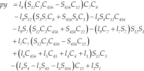
and
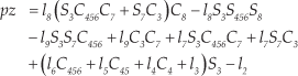
Where sθi = sinθi, cθi = cosθi, sθij = sin(θi+θj), cθij = cos(θi + θj), sθijk = sin(θi + θi + θk), and cθijk = cos(θi + θj + θk).
Once the forward kinematics is obtained, the next section presents the solution to the inverse kinematics for the legs in Sagittal and Frontal planes.
3. Inverse Kinematics
This section is concerned with finding the solution to the inverse kinematics problem, which consists of determining the joint variables in terms of the end effector position and orientation. It is commonly known in the literature that for open kinematic chains, the determination of closed-form equations for the inverse kinematics represents a greater challenge than the forward kinematics [27].
3.1 Inverse Kinematics in the Sagittal Plane
Figure 2 shows the right leg in the Sagittal plane that describes the motion of the humanoid biped robot, where the base coordinate is at the centre of the toe joint. Note that δ x and δ y are the differential step positions, while (X3,Z3), (X1, Z1) and (X0, Z0) denote the position for the waist, ankle and toe, respectively.

Right leg inverse kinematics
The approach that this paper follows for finding the inverse kinematics solution for the right leg in the Sagittal plane consists of determining the joint angle for the knee θ4, given the global position for the hip and ankle. This work considers that the trajectories of the ankle and hip in the Sagittal plane are known.
Applying the law of cosines to the triangle bounded by l4 and l5 in Figure 2, results in
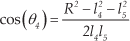
By further using the trigonometric identity atan2, results in the solution for θ
4

where:

The ankle angle θ
5
(see Figure 2) is obtained by adding angles θ
a
and θ
b
as follows


and

After calculating the ankle and knee angles, the next step is to calculate the hip angle. From geometry it is possible to know that in order to keep the hip of the robot in a vertical position, the ankle, knee and hip angles need to sum zero. Hence, the hip angle θ3 can be determined as follows

Following the same procedure, the toe angle toe θ3 is

where:

The inverse kinematics for the left leg can be solved with a similar approach as those for the right leg, namely


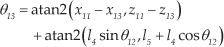
and

Where θ11, θ12, θ13, and θ16 represent the angles of the waist, knee, ankle and toe respectively, in the left leg.
3.2 Inverse Kinematics in the Frontal Plane
Figure 3 shows the model of the motion of the humanoid biped robot in the Frontal plane. Note that the base coordinate is at the centre of the ankle, where θ2 and θ7 are the angle in the waist and ankle joint for the right leg, respectively. Likewise, θ10 and θ15 represent the angle in waist and ankle for the left leg, respectively. Additionally, h represents the height of hip joint, and ls is the width of a step.

Inverse kinematics in Frontal plane
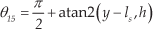
Note that θ7 has been found with trigonometric identities, by using the triangle formed at the articulation of the ankle, hip height and half the width of the step, namely

In order to keep the hip of the robot in a vertical position, the ankle, knee and hip angles need to sum π. Therefore, the hip angle θ2 can be determined as follows;

A similar procedure has been used to find the angles θ15 and θ10, for ankle and waist joints in the left leg.
and

Where y represents in Eqs. (19) and (21) the trajectory followed by the hip joint, which is a periodic function and is further introduced in Section 4. Once the forward and inverse kinematics have been determined, the next step consists in proposing all the trajectories that are to be followed by each joint.
4. Trajectory Planning
This work intends to tackle the problem of controlling the biped robot in order to produce walking gait, when the legs follow a desired trajectory. Therefore, it is essential to obtain the desired joint space trajectory given by the Cartesian space trajectory [28]. The points on the following periodic functions are used to determine the rotation angle and thus, calculate the torque of the joints.


and

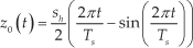
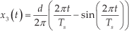
Note that Equations (23) to (28) show the periodic functions that describe the biped moving trajectory in the Sagittal plane, while Eq. (29) is the trajectory for the knee in the Frontal plane. Figure 4 shows the trajectory followed by the right leg for one step and the parameters used in the gait trajectory from Eqs. (23) to (28), where s is the length of one step, sh is the height between the sole of the foot and ground, d is the hip moving distance, h is the height of hip joint, Ts is the period of one step, and t denotes time.

Parameters used in trajectory periodic functions
5. Dynamics of Humanoid Biped Robot
The approach followed in this paper applies the principles of Lagrangian dynamics for determining the gait locomotion equations for obtaining the torque in each joint of the biped robot. If we recall that in the absence of friction and other disturbances, the Lagrangian L (q, q̇) of a mechanical system is defined by
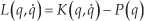
Where K (q, q̇) y P (q) represent the kinetic and potential energy of the system, respectively. Note that q ε ℝ
n
represents the vector of generalized coordinates of the system, and
The equation of motion of Euler-Lagrange for the humanoid biped robot is given by:
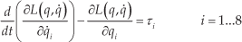
Where τ
i
. ε ℝ
n
is the vector of external generalized forces acting on each joint of robot, qi represents the position of link i, and q̇i is the velocity of link i. The kinetic energy for the humanoid robot in the Sagittal plane is calculated by

Where Ii represents the inertia for link i, mi represents the mass of link I and vi is the velocity of link i. The potential energy for each link can be written as

Where g is the gravity vector in the inertial frame and the vector rci represents the coordinates of the centre of mass of link i.
The Euler-Lagrange motion equations provide the following dynamic model [20]:
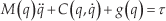
Where M (q) ε ℝ nxn is the inertia matrix, which is symmetric and defined as positive, C(q, q̇)ε ℝ n is the vector of centrifugal and Coriolis forces, and g (q) ε ℝ n is the vector of gravitational forces.
To calculate the position and torque in each joint, this paper considers a PD control law with gravity compensation [29], given by the equation

Where Kp, Kv ε ℝ
nxn
represent the symmetric positive definite matrices, q̂ is the position error and is defined as q̂ = qd – q, where qd is the desired position, and 

PD control with gravity compensation for humanoid robot
In this study the motion of the humanoid robot is described in the dynamic model as consisting of two planes, divided by the Sagittal and Frontal planes. This planar model can be compared to a chain of n rigid links. In the case of the Sagittal plane, the motion of the humanoid biped robot is modelled by the position (X, Z) as shown in Figure 6, where the base coordinate is at the centre of the waist, (x0, z0) is the position of point of support, and (xf, zf) is the position of the free toe end.

Sagittal plane view of the humanoid robot
In the case of Frontal plane, the motion is defined by the position (Y, Z) as shown in Figure 7, where the base coordinate is at the centre of the waist, (y0, z0) is the position of the point of support and (yf, zf) is the position of the free toe end. For both planes, the dynamic equations for the humanoid biped robot were presented in [30].

Frontal plane view of the humanoid robot
6. Numerical Example and Simulation
This work used Maple for producing the numerical examples of the analytical solutions to the kinematics, trajectory planning and dynamics of the humanoid robot. In addition, this paper used SolidWorks and the SimMechanics toolbox from MATLAB for modelling and simulating mechanical systems that use the standard Newtonian laws [31].
6.1 Inverse Kinematics and Trajectory Planning
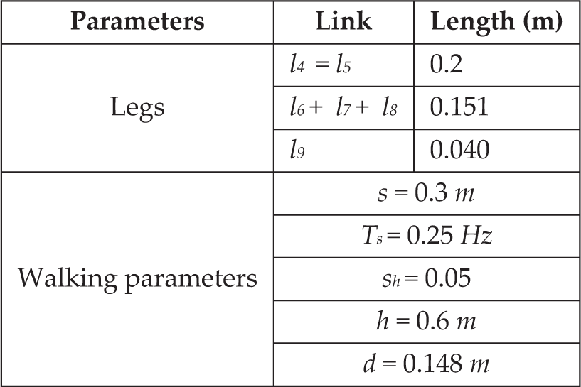
Table 3 shows the parameters used for the inverse kinematics and trajectory planning in the numerical examples and motion simulations as shown in Fig 2.
Dimensional and gait parameters of the humanoid robot
Substituting the parameters from Table 3 into Eqs. (23) to (29), Figure 8 shows the desired gait trajectory for the hip, left, and right foot in dotted, solid and dashed plots respectively, for five steps and with a maximum height of 0.3 m.
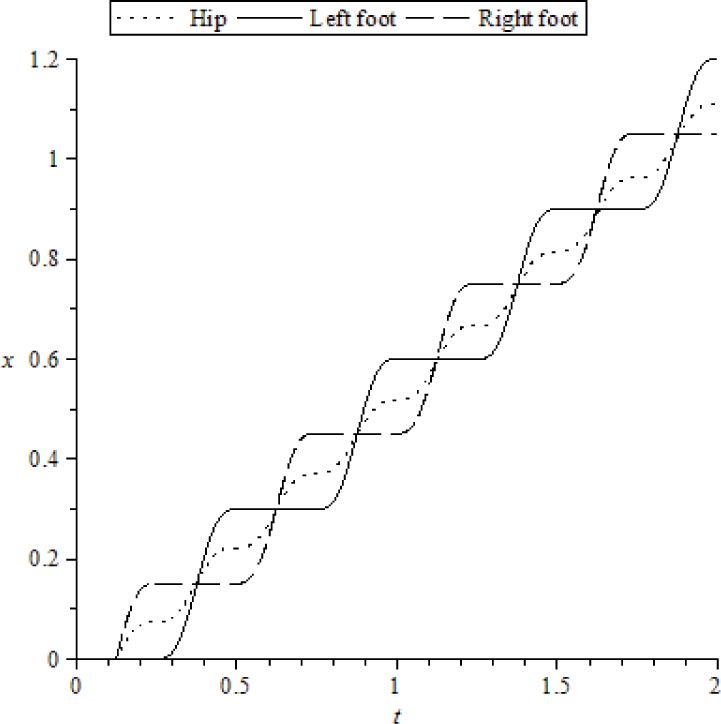
Given trajectory for periodic walking
Figure 9 presents the desired feet trajectory for five steps. Note that the maximum height between the sole and the feet is considered to be 0.05 meters.
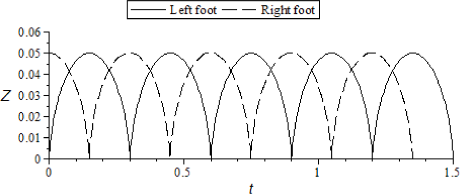
Given trajectory for feet in periodic walking
Considering the previously presented gait trajectories in Figures 8 and 9, the position of the right and left legs in the Sagittal plane for joints q3, q4, q5, q11, q12 and q13 is illustrated in Fig. 10 for periodic walking by evaluating Eqs. (6) to (18) for the inverse kinematics in the Sagittal plane. Note that Figure 10 shows the displacement of q5 and q13 for the ankle, q4 and q12 for the knee, and q3 and q11 for the waist for a gait period.

Calculated position in Sagittal plane
To verify the analytical results obtained in this paper, SolidWorks and SimMechanics Tool box of MATLAB are used. The model created with the aid of SolidWorks is exported to SimMechanics, where the dynamic simulation is performed. Figure 11 shows the plots for the right and left leg in the Sagittal plane for four steps with a gait period of 0.25. Note that the result given by SimMechanics is similar to the result shown for the numerical example in Figure 10. The simulation parameters (e.g. inertia, mass, and centre of gravity) are imported from the SolidWorks CAD model as shown in Tables 4 and 5.

Leg position simulation in Sagittal plane
Dynamics parameters of the right leg in Sagittal plane

Dynamics parameters of the right leg in the Frontal plane.

Figure 12 is presented in order to validate the inverse kinematics in the Frontal plane by using Eqs. (19) to (22) to obtain the configuration of the q7 waist joint with a maximum slope of 0.5π. Furthermore, the figure shows the lateral motion in the q2 ankle joint with a maximum slope of π.
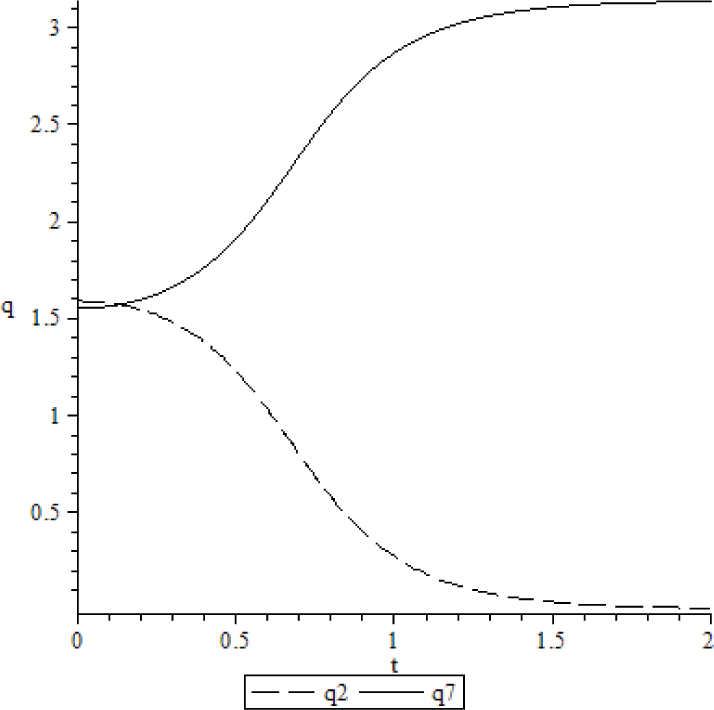
Calculated position trajectory for the q2 joint in waist and q7 joint in ankle for periodic walking
Following the same approach, Fig. 13 shows the simulation results for the Frontal plane. This simulation represents the lateral motion in the legs for the humanoid; note that the plot is similar to Fig. 12, showing plausibility between the simulation and analytical results.

Simulation in Frontal plane of legs trajectories
6.2 Dynamics
The calculation of the torque for each joint in the Sagittal plane is approached by using Eqs. (30) to (36). Consider a case (i) in which the desired joint positions qdi for the link i, are chosen as qd1 = π/6, qd2 = 0, qd3 = 0 and qd4 = 0. Table 4 shows the dynamics parameters used in this numeric calculation (see Fig. 6), all values in the Table 4 were obtained from the SolidWorks CAD model. It is possible to see in Figure 14 that the desired position for qd1 = π/6 is achieved at approximate 8 seconds with a torque of 2.8 Nm (see Fig. 15). In addition, Figure 14 shows the position for the other joints qd2 = 0, qd3 = 0 and qd4 = 0, note that the position results are close to zero.

Calculated position of joints q1, q2, q3 and q4 for case (i)

Calculated torque of joints q1, q2, q3 and q4 for case (i)
Figure 15 represents the torque required for q1 in order to achieve the desired position qd1 for case (i). The same Figure shows the T2, T3 and T4 torques for the joint q2, q3 and q4. Note that the torque T2 is negative since it is opposite to the motion of q1.
Consider now a case (ii) in Figures 16 and 17 that presents the results for a numeric example when the trajectory is a walking period given by Eqs. (30) to (36), when qd1 =0.0125(8π-sin(8πt))/π, qd2=0, qd3=0 and qd4=0. Note in Fig. 16 that the maximum position of the trajectory for q1 when the desired position is qd1 = 0.9 rad is reached in 10 seconds with a corresponding torque of 4.153 Nm (see Fig. 17). Furthermore, the Figures show the position and torque for the joint q2, q3 and q4, where it is possible to see that their results are close to zero. Note that the torque T2 is negative because opposes the motion of q1.

Calculated position of joints q1, q2, q3 and q4 for case (ii)

Calculated torque of joints q1, q2, q2 and q4 for case (ii)
Similarly to the previous simulation, with the use of Eqs. (30) to (36), it is possible to perform the calculation of the torque for each joint for the Frontal plane. The Table 5 shows the dynamics parameters used in this calculation for the Frontal plane (see Fig. 7), which are obtained from a Solidworks CAD model.
Consider now a case (iii) where the desired positions are qd1=π/12 and qd2=0. Note that Figure 18 presents the position for q1 to achieve the desired position qd1=π/12, which is reached at approximate 3.5 seconds with a torque of 2.3 Nm (see Fig. 19). Furthermore, Fig. 18 and Fig. 19 show the position of joint q2 and torque T2, respectively. Note that the motion of this joint is performed in order to achieve the desired position for joint q1.

Calculated position of joints q1 and q2 for case (iii)

Calculated torque of joints q1 and q2 for case (iii)
7. Conclusions
This paper presented a new architecture for a biped robot with seven DOF per each leg and an additional DOF that imitates the toe joint.
This work presented the forward kinematics using the DH convention, while the inverse kinematics were approached by decoupling the Frontal and Sagittal planes, resulting in a simplified model that led to closed-form equations for the leg position and orientation.
By considering periodic gait functions, the paper obtained leg trajectories for determining the biped motion and the required torque for each joint. The principle of Lagrangian dynamics applied a PD control law with gravity compensation in order to control the desired trajectories and to find the torque required by the joints.
Several numerical examples were compared to motion and dynamic simulations, which verified the analytical results.
Future work after this paper will focus on the velocity and acceleration analysis, followed by a singularity analysis in order to identify and eliminate the singular configurations through redundancy. A prototype will be manufactured in order to test alternative algorithms for the gait stability control.