Bio-inspired controller achieving forward speed modulation with a 3D bipedal walker

Abstract

Despite all the effort devoted to generating locomotion algorithms for bipedal walkers, robots are still far from reaching the impressive human walking capabilities, for instance regarding robustness and energy consumption. In this paper, we have developed a bio-inspired torque-based controller supporting the emergence of a new generation of robust and energy-efficient walkers. It recruits virtual muscles driven by reflexes and a central pattern generator, and thus requires no computationally intensive inverse kinematics or dynamics modeling. This controller is capable of generating energy-efficient and human-like gaits (both regarding kinematics and dynamics) across a large range of forward speeds, in a 3D environment. After a single off-line optimization process, the forward speed can be continuously commanded within this range by changing high-level parameters, as linear or quadratic functions of the target speed. Sharp speed transitions can then be achieved with no additional tuning, resulting in immediate adaptations of the step length and frequency. In this paper, we particularly embodied this controller on a simulated version of COMAN, a 95 cm tall humanoid robot. We reached forward speed modulations between 0.4 and 0.9 m/s. This covers normal human walking speeds once scaled to the robot size. Finally, the walker demonstrated significant robustness against a large spectrum of unpredicted perturbations: facing external pushes or walking on altered environments, such as stairs, slopes, and irregular ground.

1. Introduction

Mobile robots hold the promise of better integration of robotics into our everyday life. However, they are usually restricted to environments adapted to their mobility. Humanoid robots offer an interesting perspective in this context, since their body, which roughly similar to our own, is potentially perfectly adapted to our world, designed for humans (Schaal, 2007). In addition, they offer the possibility to manipulate tools designed to comply with human dexterity, so that these tools do not need to be adapted for the robot (Fitzpatrick et al., 2016). This is particularly appealing in contexts where the robot is expected either to take over a human laborious duty or to co-work in synergy with human operators.

Nowadays, these robots skills are still far from reaching the level of the human ones, thus preventing them from being used routinely. This is especially true regarding locomotion. The most popular methods developed to achieve dynamic walking rely on the zero-moment point (ZMP) as an indicator of gait feasibility (Vukobratovic and Borovac, 2004). The ZMP can then be used to generate walking patterns guaranteeing dynamic stability at every moment during the gait. Many locomotion experiments have been conducted successfully using this indicator, for example with ASIMO (Chestnutt et al., 2005) or with the HRP-2 platform (Kaneko et al., 2002).

However, there are several shortcomings related to these ZMP-based bipedal controllers, notably energy inefficiency (Dallali, 2011). Furthermore, the generated pattern gaits look quite unnatural (low waist position, permanent knee bending, feet kept parallel to the ground, etc.) and the resulting walking speed is typically much slower than that achieved by a healthy human displaying the same morphology (Kurazume et al., 2005; Sardain and Bessonnet, 2004). In particular, ZMP-based controller synthesis usually requires to avoid singular configurations,thus preventing the leg to reach full extension during the stance phase (Kurazume et al., 2005). This has a direct impact on the energy consumption, since a bent knee requires a torque to be maintained, in order to balance the body static and dynamic forces. Some contributions however managed to address this problem (Ogura et al., 2006).

Another concept frequently used to achieve dynamic walking is the inverted pendulum model (IPM). In its most basic version, the IPM models the biped as a single point mass with contact forces acting at the feet level, in order to produce desired motions for the center of mass (COM). The IPM can then possibly be used to control the ZMP (Faraji et al., 2014a,b). The linear inverted pendulum (LIP) is a special case of the IPM where the point mass is constrained to move in a plane of constant height (Razavi et al., 2017).

The limit cycle walking concept relaxes the need to guarantee the local stability at all times of the gait. It treats the gait as a limit cycle and investigates its global stability (Hobbelen and Wisse, 2007). (Quasi-)Passive walkers are successful implementations of this concept (Collins and Ruina, 2005; Hobbelen et al., 2008; McGeer, 1990). Although they display human-like gait patterns and require zero (or little) energetic consumption, they are usually limited to very controlled environments, since they usually lack control variables to modulate the gait or to resist perturbations like obstacles or collisions.

Another avenue to explore the limit cycle walking concept is through the development of so-called bio-inspired walkers. Here, bio-inspiration means that the principles governing the design of the walker’s body and/or controller rely on concepts identified in humans. In particular, the seminal paper of Geyer and Herr (2010), further extended in Song and Geyer (2015), developed a bipedal model being actuated by a human-like neuromuscular model. Using reflexes to drive these muscles, they could reproduce human-like walking_ patterns and leg kinematics, and predict muscle activation patterns similar to human walking experiments. In addition, the simulated viscoelastic properties of these virtual muscles provided robustness to external perturbations.

This approach was further extended to provide realistic motions of 3D animated characters (Geijtenbeek et al., 2013; Wang et al., 2012). Interestingly, part of this model was also adapted to control a powered ankle–foot prosthesis (Eilenberg et al., 2010), thus further enhancing the bio-inspired framework. In Van der Noot et al. (2015a), we brought this controller to a real humanoid robot. When external assistance was provided to the lateral balance, the robot was capable of walking on a treadmill.

However, the reflex rules developed in Geyer and Herr (2010) do not feature modulation capabilities, for instance regarding the control of the forward speed. Song and Geyer (2012) solved this limitation by optimizing the many parameters of this controller to reach different forward speeds. Large speed variations requested then to run additional optimizations to find new parameter modulations between pre-optimized walking gaits.

An alternative bio-inspired gait modulation strategy requires the addition of a central pattern generator (CPG). CPGs are neural circuits capable of producing rhythmic patterns of neural activity without receiving rhythmic inputs. They feature valuable properties such as distributed control, redundancies handling, and locomotion modulation using simple control signals (Ijspeert, 2008).

While locomotor CPGs were identified in many vertebrates, their involvement in human locomotion is still a matter open to discussion (Dimitrijevic et al., 1998). Yet, computational models showed that CPGs could play a major role in human locomotion. For instance, Taga (1994) could adapt the locomotion of a bipedal model on uneven terrains, using CPG modulation. Aoi and Tsuchiya (2005) could achieve robust walking with a biped robot by recruiting nonlinear oscillators, both in numerical simulations and with a hardware platform. In Dzeladini et al. (2014), a CPG was added to the controller of Geyer and Herr (2010), in order to act as a feedback predictor and, then, to modulate the forward speed. This provided an interesting implementation of Kuo’s framework for combining feedback (i.e. reflexes) and feed-forward (i.e. CPG) pathways in the control of a periodic task (Kuo, 2002). In Paul et al. (2005), a neuromuscular model used a CPG as central element to investigate the effects of a spinal cord injury on locomotor abilities. Importantly, modeling efforts investigating the potential role of CPG in human locomotion ubiquitously display their complex intertwining with feedback mechanisms (Rossignol et al., 2006).

In the present contribution, we embrace the idea of combining a CPG and reflexes in a neuromuscular torque-based controller for bipedal locomotion. More precisely, we design a controller capable of generating robust and human-like locomotion gaits on a 3D bipedal walker. In particular, forward speed modulation is achieved through the adaptation of some high-level parameters, i.e. mainly the CPG inputs. Preliminary results of this controller (i.e. limited to the 2D sagittal plane) were already published in Van der Noot et al. (2015b).

This paper is divided as follows. In Section 2, the walking controller is extensively detailed. Then, Section 3 presents both the simulation environment and the robotic platform that was used for embodying our controller, namely COmpliant huMANoid (COMAN), a 95 cm tall humanoid robot. The controller is further extended in Section 4, in order to achieve forward speed modulation. The resulting gait features are analyzed in Section 5, while Section 6 evaluates the robustness of the controller when walking blindly in perturbed environments. Finally, Section 7 concludes the paper.

2. Controller design and architecture

Our controller is expected to provide torque references for all the joints of a bipedal walker. These torque references are computed from a bio-inspired approach: they derive from forces being produced by virtual muscles. These muscles are in turn “activated” by receiving appropriate stimulations. The coordination of these stimulations is governed by a CPG central unit. Importantly, this paper reports the successive increments performed while designing this CPG network, in order to generate the stimulation patterns governing different walking features. Combining these stimulations with virtual reflexes, robust and efficient gaits can be obtained after an optimization of the many parameters controlling both the reflexes and the CPG. The different modules developed in this controller, together with the biped embodiment, are summarized in Figure 1.

Fig. 1.

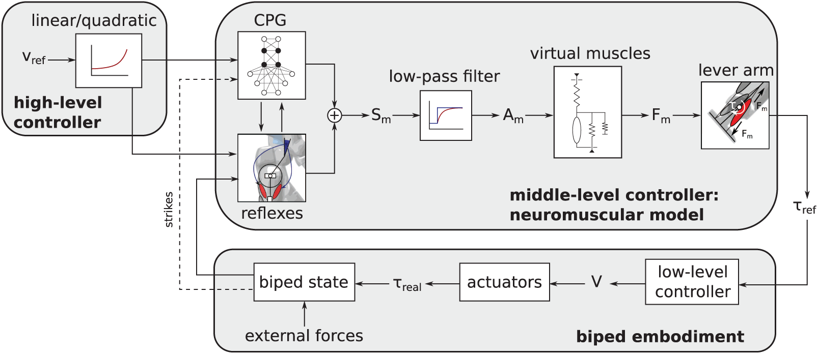
The purpose of the neuromuscular controller is to provide torque references ${\tau }_{\mathrm{ref}}$ to the biped joints when receiving sensory information from the biped state. On top of that, high-level commands are provided by the user as linear or quadratic functions of a scalar input: the speed reference $v_{\mathrm{ref}}$ . Then, the interplay between the CPG and the reflexes provides stimulation signals $S_m$ . They are later converted into activations $A_m$ controlling the virtual Hill-type muscles. These muscles finally produce forces $F_m$ , converted into the joint torques via lever arms. The biped embodiment used in this contribution tracks the desired torques ${\tau }_{\mathrm{ref}}$ by feeding the actuators with appropriate voltages V. The actual torques ${\tau }_{\mathrm{real}}$ , combined with the external forces, drive the time evolution of the biped state, eventually resulting in locomotion.

2.1. Neuromuscular model

The investigated joints configuration is provided in Figure 2. This configuration fits that of the COMAN robot (Tsagarakis et al., 2013), which served as embodiment for our experiments (see Section 3.1). This joint configuration is quite ubiquitous in humanoid robots, so that the proposed controller should be adaptable to many other humanoid robots.

Fig. 2.

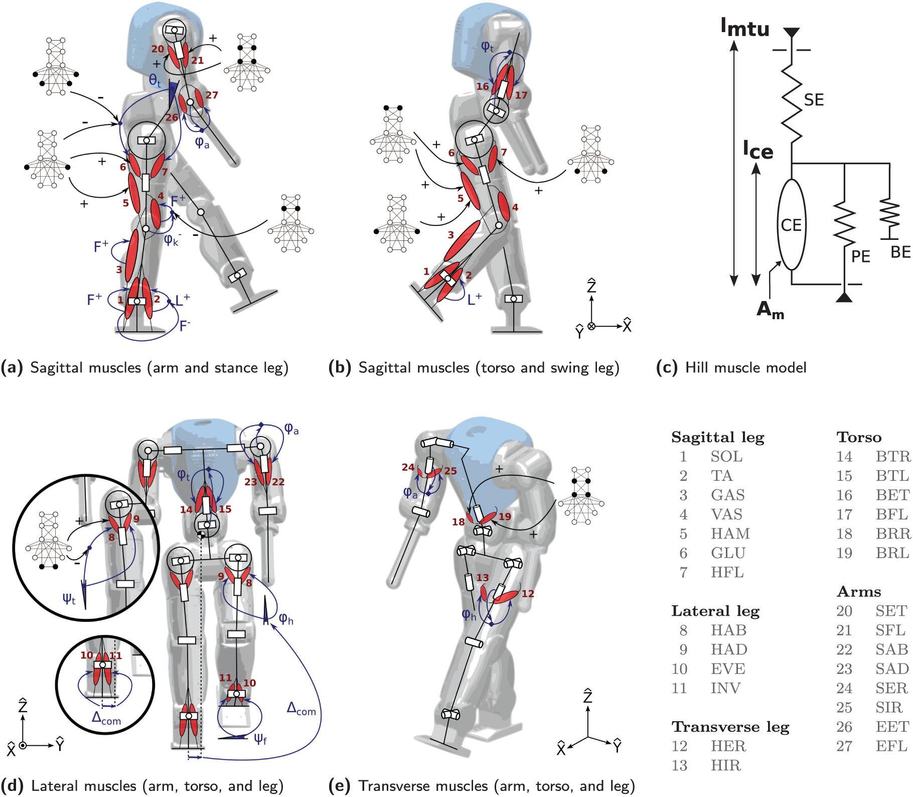
To actuate the biped’s 23 joints, the controller recruits 27 different Hill muscle models (c) acting in different planes. These muscles are commanded by a combination of reflex signals and the CPG central unit. Muscles acting in the sagittal plane are displayed in (a) and (b), those affecting the lateral plane are displayed in (d), and finally, those acting in the transverse plane are depicted in (e). See the text for further details.

To drive these joints, the robot recruits (virtual) muscles. This approach is directly inspired by the paper of Geyer and Herr (2010) and is outlined below. Different muscle groups are identified in each body part, and correspond to muscles of the actual human leg anatomy: 27 different types of muscle groups are recruited to actuate the 23 joints of the biped, as reported in Figure 2.

More precisely, each muscle group is computed as a set of equations, called the Hill muscle model (Hill, 1938) and pictured in Figure 2c. Each muscle tendon unit (MTU) consists of two main elements: a contractile element (CE) and a series elastic element (SE). Two additional passive elements further engage when the muscle state is outside its normal operation range: the parallel elastic element (PE) and the buffer elasticity element (BE). The length $l_{\mathrm{mtu}}$ of each MTU is computed by geometrical relationships involving the joint angles and the MTU attachment points. The length of CE $l_{\mathrm{ce}}$ is integrated based on $l_{\mathrm{mtu}}$ and on the muscle activation $A_m$ , which is detailed later. Then, the deformation of SE (i.e. the length $l_{\mathrm{se}}$ , computed as $l_{\mathrm{se}}=l_{\mathrm{mtu}}-l_{\mathrm{ce}}$ ), provides a direct computation of the force $F_m$ generated by the muscle. Finally, this force $F_m$ is multiplied by the muscle lever arm $r_m$ to generate a torque contribution to the corresponding joint. For bi-articular muscles (i.e. GAS and HAM in Figure 2a and b), a single muscle provides two torque contributions with two different lever arms. The full implementation of these equations can be found in Appendix B.

In sum, this musculoskeletal model provides joint torques through virtual muscle forces and attachment points. Thus, instead of directly controlling the torques, we rather control each MTU through input signals called muscle activations $A_m$ . They are related to neural inputs $S_m$ called stimulations, using a first-order low-pass filter capturing the excitation–contraction dynamics (see Figure 1 and Appendix B.2). The following sections detail how the stimulations $S_m$ of each muscle are computed.

2.2. Frequency and phasing signal construction

Our controller uses both CPG signals and reflexes to drive the muscles. The combination between these two types of signals mainly follows a proximo-distal gradient. In other words, muscles close to the hips are mainly controlled by CPG signals (feed-forward), whereas those close to the feet are mainly driven by reflexes (feedback) (Dzeladini et al., 2014). This builds upon the rationale that distal muscles are more impacted by external perturbations such as ground interactions (Daley et al., 2007).

Our CPG is designed as a 12-neuron network of Matsuoka oscillators (Matsuoka, 1985, 1987). These are bio-inspired artificial oscillators, capturing the mutual inhibition between half-centers located in the spinal cord. They also have interesting properties. Indeed, they feature stable limit cycles, have a low computational cost and are easy to integrate with sensory feedback signals. In this contribution, the CPG network is divided into two main parts (see Figure 3). The first is in charge of providing the main frequency and phasing of the gait cycle. Its neurons are denoted with a number (from 1 to 4) and are called “rhythm generator” neurons (RG). The second layer relies on the RG neurons to generate signals shaping the patterns of muscle stimulations. The corresponding neurons are denoted with a letter (from A to H) and are called “pattern formation” neurons (PF). This two-layered division is inspired by the two-level CPG biological structure proposed by McCrea and Rybak (2008). In that contribution, the authors report several experiments of fictive locomotion in the decerebrated cat that can be reproduced with this particular CPG architecture.

Fig. 3.

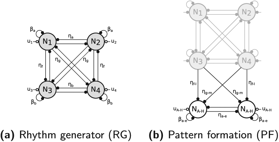
The central pattern generator (CPG) network is built by assembling two types of components: (a) the rhythm generator (RG) part (four fully connected Matsuoka neurons) and (b) a pair of pattern formation neurons (PF) driven by the RG neurons. The vertical symmetry corresponds to the left/right legs symmetry.

During the gait cycle, the strike impact is a crucial moment where the load is quickly transferred from one leg to the other. Simultaneously, a large effort is requested from the new stance leg to prevent the torso from collapsing forward, as a result of this large impact. Therefore, it is critical for the CPG network phase to be synchronized with the foot strike, so that it provides large stimulations right after impact. During the following loading response, the leg leaving the stance phase must also provide significant effort, in order to propel the body and prepare the swing phase through proper hip flexion and foot push-off. Next, before the following strike, hip moments are less significant in both legs. Indeed, the stance leg already absorbed the main shock and only needs to maintain the torso orientation, whereas the swing leg mainly relies on ballistic motion. As a consequence, it is convenient to divide the gait cycle into four stages. Two stages are triggered by foot strikes from both legs, whereas the two others approximately start during mid-stance. This decomposition is similar to the high-level control states presented in Yin et al. (2007) or in Wang et al. (2012).

The CPG RG part is thus constructed with four neurons, one for each stage. More precisely, we use four fully connected Matsuoka neurons (Matsuoka, 1985, 1987). This structure is displayed in Figure 3a.

The Matsuoka equations governing this CPG are detailed below. Each neuron $N_i$ main state is captured by its so-called firing rate $x_i$ . Its evolution with time is governed by

$${ẋ}_i=\frac{1}{\tau }\left(-x_i-{\beta }_j{v}_i-\sum {\eta }_k{\left[x_l\right]}^{+}+u_i\right)$$

(1)

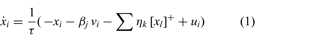
where $\tau$ is the time constant for the rate of discharge, $v_i$ is the self-inhibition modulated by an adaptation constant ${\beta }_j$ , and $u_i$ is the external input.

Finally, the connection strengths ${\eta }_k$ govern mutual inhibition, i.e. the fact that the activation of a given neuron decreases when another is active. It is captured by the function ${\left[•\right]}^{+}=max\left(0,•\right)$ , so that only positive firing rates are considered for inter-neuron inhibition. The self-inhibition state variable is governed by

$${\stackrel{.}{v}}_i=\frac{1}{{\gamma }_j\tau }\left(-v_i+{\left[x_i\right]}^{+}\right)$$

(2)

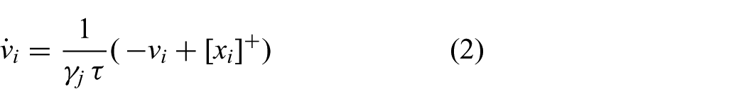
whose time constant is related to that of Equation (1) through the adimensional parameter ${\gamma }_j$ .

In (1) and (2), the index i corresponds to the neuron index, whereas the gains ${\beta }_j$ , ${\eta }_k$ , and the neurons $x_l$ are specified in Figure 4. Finally, ${\gamma }_j$ takes thesame index as ${\beta }_j$ . These equations are fully developed in Appendix C.

Fig. 4.

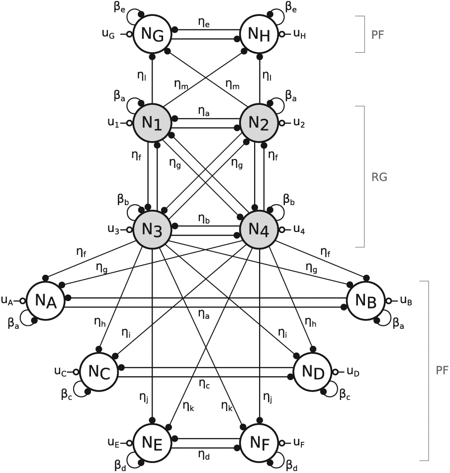
Full central pattern generator (CPG) network: inter-neuron excitations are indicated with an empty circle, whereas plain circles represent inhibitions. The “rhythm generator” neurons (RG, shaded) affect the “pattern formation” neurons (PF), but not vice versa. The network vertical symmetry produces motor commands for both body sides (legs and arms). The neurons’ main contributions are as follows: $N_{\left\{1-4\right\}}$ , rhythm generator and upper-body control; $N_{\left\{A,B\right\}}$ , knee bending and torso sagittal stabilization; $N_{\left\{C,D\right\}}$ , hip flexion; $N_{\left\{E,F\right\}}$ , torso lateral stabilization; $N_{\left\{G,H\right\}}$ , late swing leg retraction. The corresponding muscular activations are highlighted with plain circles in Figure 2. The full CPG equations are provided in Appendix C.

Interestingly, the time constant $\tau$ is inversely proportional to the CPG frequency. This provides useful access for modulating the gait frequency.

Regarding phase locking, different models exploited the capacity of CPGs to achieve entrainment, i.e. to synchronize their firing pattern with stimulations generated by the actuated body and/or its environment. In particular, Aoi et al. (2010) developed a locomotor CPG model to achieve bipedal locomotion, also by recruiting a two-level CPG biological structure (i.e. combining RG and PF networks). In this model, phase resetting was applied to the RG layer, based on foot-contact information. CPG entrainment was also achieved using Matsuoka oscillators. For instance, in de Rugy and Sternad (2003) and Ronsse et al. (2009), this mechanism was investigated for uni- and bi-manual upper-limb movements, whereas Paul et al. (2005) and Taga (1994) investigated locomotion. Here, a similar mechanism generating short excitations modulations at foot strike is used. Basically, all the excitations $u_i$ consist in a tonic excitation of $u=1$ . Then, if a neuron $N_i$ is too slow (i.e. not firing while the corresponding phase already started) or too fast, its excitation $u_i$ is shortly modulated as reported in Appendix D. Combining it with the time constant $\tau$ modulation, this guarantees that the CPG and the walker display the same frequency, while staying in phase with feet strikes.

The four RG neurons N₁, N₂, N₃, and N₄ are the central elements of the whole CPG network in Figure 4. Their typical firing rates temporal evolutions are pictured in Figure 5. In the following sections, this network is incremented with the PF neurons.

Fig. 5.

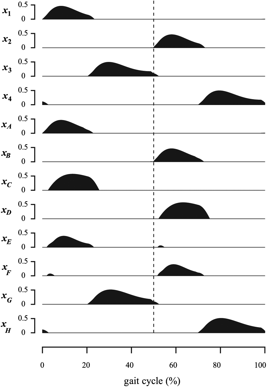
Time-evolution of the 12 neurons’ firing rates of Figure 4 over one gait cycle ( $0\%$ and $100\%$ correspond to right foot strikes, the dashed line corresponds to left foot strike). These signals are obtained during one typical gait cycle of the locomotion resulting from the controller used in most of the results of this paper (called reference controller), with a speed reference of 0.65 m/s.

2.3. Leg sagittal stance control

The four RG neurons network determines the CPG frequency and phase synchronization. In order to send appropriate stimulations to the muscles, this network is further incremented with pairs of PF neurons. These receive inputs from the RG neurons but not the other way round. This is achieved with the unidirectional structure displayed in Figure 3b.

To generate the CPG contribution to a particular muscle stimulation $S_m$ , the different CPG outputs $y_i$ are computed as detailed in Appendix E.1. They mainly consist of extracting the positive firing rate of a PF neuron $x_j$ (i.e. $y_i={\left[x_j\right]}^{+}$ ). Then, the CPG contribution to a particular stimulation is computed as $S_m=\sum k_i{y}_i$ , where $k_i$ is a gain.

As mentioned earlier, fast hip muscle reactions are required after strike impact to prevent the torso from collapsing forward. This is provided by the gluteus (GLU) and hamstring (HAM) muscle groups. Therefore, neurons being aligned (i.e. firing at the same time) with the N₁ and N₂ neurons of the RG structure are requested, so that they can quickly fire right after strike. This is the purpose of the two neurons $N_A$ and $N_B$ (see Figure 4). They are in charge of providing the requested stimulation patterns. In order to keep them aligned with N₁ and N₂, similar weights are used for the self and mutual inhibitions, as well as for the time constant gains. As can be seen in Figure 5, their firing signals ( $x_A$ and $x_B$ ) are indeed well aligned with x₁ and x₂, as expected.

After the strike impact absorption, reflexes are activated at the hip level to maintain the torso sagittal lean angle ${\theta }_t$ close to a reference ${\theta }_{\mathrm{ref}}$ . The requested muscles are the hip flexor (HFL) and GLU muscles. As proposed in Geyer and Herr (2010), this is performed by a proportional–derivative (PD) control of the lean angle error, ${\mathrm{\Delta }}_{\mathrm{PD}}={\theta }_{\mathrm{ref}}-{\theta }_t$ . This signal generates a stimulation to one of the two antagonist hip muscles, i.e. one muscle receives a stimulation proportional to ${\left[{\mathrm{\Delta }}_{\mathrm{PD}}\right]}^{+}$ , the other to ${\left[{\mathrm{\Delta }}_{\mathrm{PD}}\right]}^{-}$ (with ${\left[•\right]}^{-}=-min\left(•,0\right)$ ). This reflex can however send contradictory signals to those generated by the CPG. To avoid this, an inhibition mechanism ruled by the CPG was implemented (see Appendix E.1).

The remaining leg sagittal muscles are distal, namely soleus (SOL), tibialis anterior (TA), gastrocnemius (GAS), and vasti (VAS) muscle groups. They are mainly controlled by similar reflexes as those reported in Geyer and Herr (2010). Most of them either combine a positive constant prestimulation (S₀) with positive/negative force feedbacks ( $F^{+∕-}$ ), or a local positive length feedback ( $L^{+}$ ). On top of that, the VAS reflex is inhibited when the knee exceeds a given threshold to prevent over-extension; or during the double support phase of the leg entering in swing phase, in order to allow knee flexion.

All the reflexes mentioned in this section are only activated during the stance phase, i.e. when the ground reaction force (GRF) vertical component under one foot is larger than an arbitrary threshold (here, 20 N). The full sagittal stance control is presented in Figure 2a. Further details about its implementation can be found in Appendix E.

2.4. Leg sagittal swing control

Because swing leg motion is less affected by external perturbations, its control mainly relies on feed-forward stimulations provided by the CPG. First, hip flexion is achieved by sending appropriate stimulations to the HFL muscle. This activation already starts in late stance, usually a bit after the contralateral foot strike, and spans during early swing. Therefore, the CPG network is augmented with a new pair of PF neurons: $N_C$ and $N_D$ . As expected, their corresponding firing rates $x_C$ and $x_D$ fire slightly after the contralateral leg strike (see Figure 5).

Approximatively at the same time, knee bending is achieved through proper HAM muscle activation. Preliminary results showed that it was actually not necessary to add a new pair of PF neurons to control it. Indeed, the corresponding stimulations usually need to be aligned with the existing neurons $N_A$ and $N_B$ . Consequently, we decided to directly shape the corresponding stimulations based on the $x_A$ and $x_B$ neurons’ firing rates.

After this initial high activity, swing mainly relies on the leg ballistic motion. Therefore, most muscles only receive the basic tonic stimulation. Regarding reflexes, only TA still receives a similar local positive length feedback ( $L^{+}$ ) as that introduced by Geyer and Herr (2010), in order to increase foot clearance with the ground.

In the late swing phase, the swing leg motion is reduced by the combined action of HAM and GLU, participating into leg retraction. This is achieved with a new pair of PF neurons: $N_G$ and $N_H$ . In contrast to other PF neurons, this new pair is connected to RG neurons N₁ and N₂, so that they are mainly aligned with N₃ and N₄.

The sagittal swing control described in this section is summarized in Figure 2b. Its full implementation is described in Appendix E.

2.5. Leg non-sagittal control

Regarding the leg control in the lateral plane, the gait cycle is only divided into two phases: the supporting and non-supporting phases. A leg supporting phase starts with the leg’s own strike and finishes with the contralateral leg strike. In other words, it corresponds to its stance phase shortened by the terminal double support phase.

During the supporting phase, the hip abductors (HAB) and adductors (HAD) muscles are mainly in charge of controlling the torso lateral lean angle ${\mathrm{\Psi }}_t$ . Similarly to the stance hip control in the sagittal plane, a pair of PF neurons is required to provide a first excitation to the new supporting leg, and prevent the torso from collapsing sideways. This is achieved by the neurons pair $N_E$ and $N_F$ , acting on the HAB muscles.

After the leg first impact, a closed-loop (i.e. reflex-based) PD controller is in charge of maintaining the torso lean angle ${\mathrm{\Psi }}_t$ close to a reference ${\mathrm{\Psi }}_{\mathrm{ref}}$ . Similarly to what was done in the sagittal plane, the CPG can inhibit the PD control contribution on the HAB muscle. This inhibition is triggered according to the CPG phase, to prevent contradictory signals between the CPG and this balance controller. In Song and Geyer (2013), a similar PD controller was proposed for the whole stance (i.e. no CPG signal is used). The introduction of the CPG first burst allows the PD control parameters governing the balance dynamics to be tuned only after shock absorbance. Indeed, closed-loop angle control appears inappropriate during the double support phase, when the weight is transferred from one leg to the other.

Lateral hip control during the non-supporting phase is inspired from the approach described in Yin et al. (2007) and used in Song and Geyer (2013). Basically, an active swing foot placement is implemented based on ${\mathrm{\Delta }}_{\mathrm{com}}$ , the lateral position of the COM, relatively to the supporting foot. First, a hip lateral reference position ${\phi }_{h,l,\mathrm{ref}}$ is computed as the output of a PD controller on ${\mathrm{\Delta }}_{\mathrm{com}}$ . Then, a second PD controller tracks this reference position with the hip lateral position ${\phi }_{h,l}$ , by sending appropriate stimulations to the HAB and HAD muscles.

Regarding lateral foot control during the supporting phase, the eversion (EVE) and inversion (INV) muscle groups are in charge of maintaining the body upright by bringing the lateral COM close to a reference position. Again, a simple PD feedback control is applied on ${\mathrm{\Delta }}_{\mathrm{com}}$ , i.e. on the same input as that used to compute the hip lateral reference ${\phi }_{h,l,\mathrm{ref}}$ of the contralateral leg. During the non-supporting phase, EVE and INV control the foot lateral orientation to keep it aligned with the horizontal, in order to prepare proper foot landing. The full leg lateral control is presented in Figure 2d.

Finally, the hip transverse joint is controlled by the hip external (HER) and internal (HIR) rotator muscle groups. The generation of straight motion simply requires to maintain this joint in its homing position. Our control is illustrated in Figure 2e. All the non-sagittal control rules are fully detailed in Appendix E.

2.6. Upper-body control

Upper-body control is less critical during walking. In fact, preliminary experiments revealed that freezing the upper-body joints would not prevent stable walking from being achieved. However, this resulted in slower gaits, with higher energetic consumption in the lower limbs.

The rationales governing upper-body motion in unconstrained human walking is still not clear either. For instance, Collins et al. (2009) explored whether the extra cost required to swing the arms could lead to potential benefits in the lower limbs. These experiments showed that voluntarily holding the arms required $12\%$ more metabolic energy.

Consequently, our controller also implements arm swing motion in the sagittal plane. More precisely, the shoulder flexion (SFL) and extension (SET) muscles are stimulated by appropriate CPG neurons, in order to be in phase with the gait cycle. For the sake of simplicity, the RG neurons were directly used to drive the corresponding muscles. Note, however, that extra PF neurons might further be added for the upper body, in a similar way as for the lower body. Here, SFL and SET stimulations are designed to be in phase with the contralateral leg motion.

The other arm muscles are the elbow extension (EET) and flexion (EFL) muscle groups, the shoulder abduction (SAB) and adduction (SAD) muscle groups, and the shoulder internal (SIR) and external (SER) rotation muscle groups. They are all controlled with a simple feedback controller to maintain a constant position.

Similarly to the arms swinging motion, the four RG neurons are used to control the torso transverse joints with the back rotation right (BRR) and left (BRL) muscle groups. The remaining torso muscle groups, i.e. back tilt right (BTR) and left (BTL), back flexion (BFL), and extension (BET), use again PD control on their respective joints to stabilize the homing position. All these rules are summarized in Figure 2 and fully described in Appendix E.3.

2.7. Walk initialization

Walk initiation requires the walker to move its COM on top of one of its feet. This is achieved with the muscle control scheme proposed in Heremans et al. (2016). Basically, a full-body compliant force controller uses virtual feedback forces applied to the COM to generate appropriate torques at the joint level (Hyon et al., 2007). Then, the muscle model presented in Appendix B is inverted to obtain the corresponding muscle stimulations. This controller only requires the horizontal coordinates $\left(X_{\mathrm{init}};Y_{\mathrm{init}}\right)$ of the target COM position. These coordinates are optimized as presented in Table 1.

Table 1.

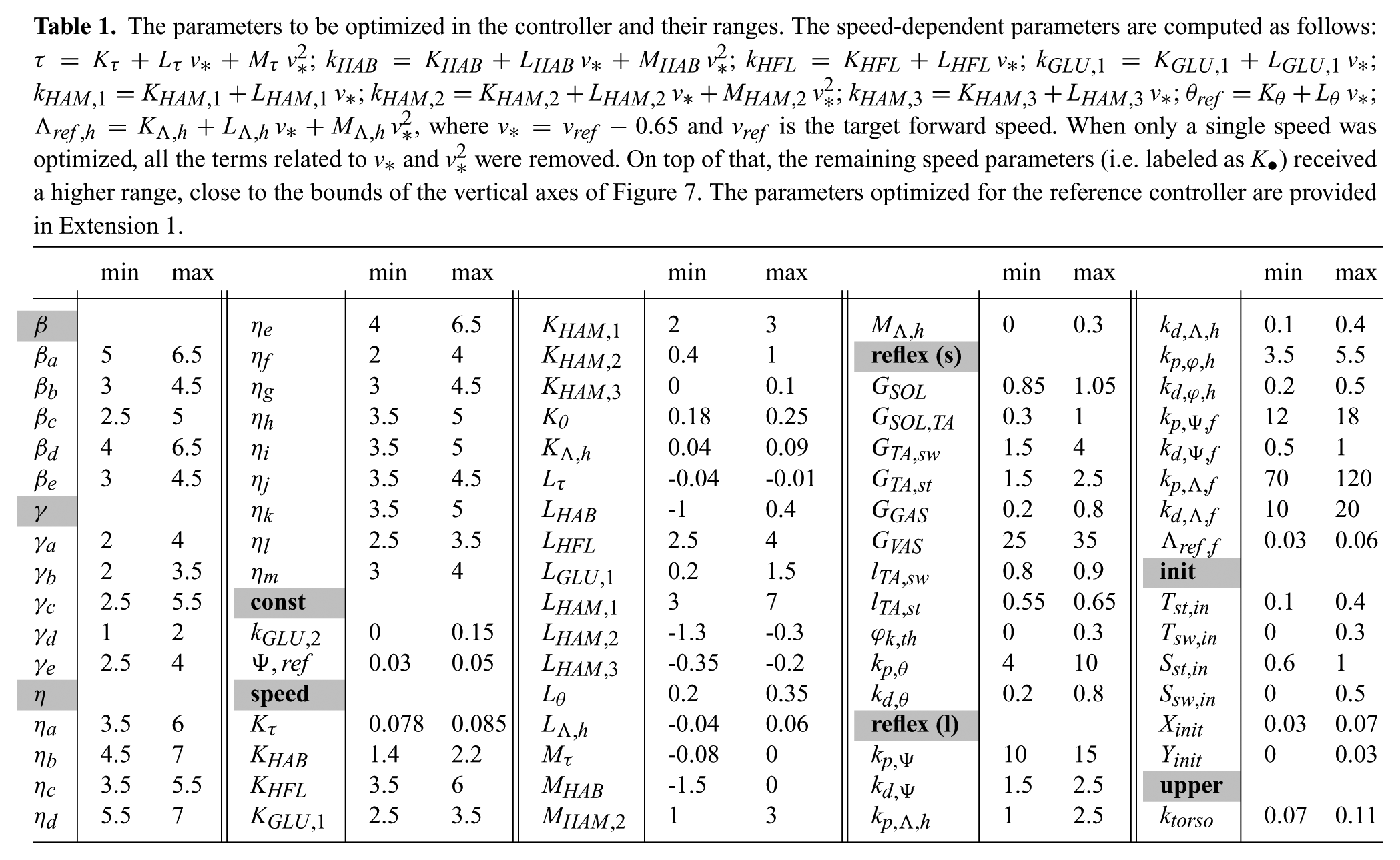
The parameters to be optimized in the controller and their ranges. The speed-dependent parameters are computed as follows: $\tau =K_{\tau }+L_{\tau }{v}_{*}+M_{\tau }{v}_{*}^2$ ; $k_{\mathrm{HAB}}=K_{\mathrm{HAB}}+L_{\mathrm{HAB}}{v}_{*}+M_{\mathrm{HAB}}{v}_{*}^2$ ; $k_{\mathrm{HFL}}=K_{\mathrm{HFL}}+L_{\mathrm{HFL}}{v}_{*}$ ; $k_{\mathrm{GLU},1}=K_{\mathrm{GLU},1}+L_{\mathrm{GLU},1}{v}_{*}$ ; $k_{\mathrm{HAM},1}=K_{\mathrm{HAM},1}+L_{\mathrm{HAM},1}{v}_{*}$ ; $k_{\mathrm{HAM},2}=K_{\mathrm{HAM},2}+L_{\mathrm{HAM},2}{v}_{*}+M_{\mathrm{HAM},2}{v}_{*}^2$ ; $k_{\mathrm{HAM},3}=K_{\mathrm{HAM},3}+L_{\mathrm{HAM},3}{v}_{*}$ ; ${\theta }_{\mathrm{ref}}=K_{\theta }+L_{\theta }{v}_{*}$ ; ${\Lambda }_{\mathrm{ref},h}=K_{\Lambda ,h}+L_{\Lambda ,h}{v}_{*}+M_{\Lambda ,h}{v}_{*}^2$ , where $v_{*}=v_{\mathrm{ref}}-0.65$ and $v_{\mathrm{ref}}$ is the target forward speed. When only a single speed was optimized, all the terms related to $v_{*}$ and $v_{*}^2$ were removed. On top of that, the remaining speed parameters (i.e. labeled as $K_{•}$ ) received a higher range, close to the bounds of the vertical axes of Figure 7. The parameters optimized for the reference controller are provided in Extension 1.

	min	max		min	max		min	max		min	max		min	max
$\beta$			${\eta }_e$	4	6.5	$K_{\mathrm{HAM},1}$	2	3	$M_{\Lambda ,h}$	0	0.3	$k_{d,\Lambda ,h}$	0.1	0.4
${\beta }_a$	5	6.5	${\eta }_f$	2	4	$K_{\mathrm{HAM},2}$	0.4	1	reflex (s)			$k_{p,\phi ,h}$	3.5	5.5
${\beta }_b$	3	4.5	${\eta }_g$	3	4.5	$K_{\mathrm{HAM},3}$	0	0.1	$G_{\mathrm{SOL}}$	0.85	1.05	$k_{d,\phi ,h}$	0.2	0.5
${\beta }_c$	2.5	5	${\eta }_h$	3.5	5	$K_{\theta }$	0.18	0.25	$G_{\mathrm{SOL},\mathrm{TA}}$	0.3	1	$k_{p,\mathrm{\Psi },f}$	12	18
${\beta }_d$	4	6.5	${\eta }_i$	3.5	5	$K_{\Lambda ,h}$	0.04	0.09	$G_{\mathrm{TA},\mathrm{sw}}$	1.5	4	$k_{d,\mathrm{\Psi },f}$	0.5	1
${\beta }_e$	3	4.5	${\eta }_j$	3.5	4.5	$L_{\tau }$	−0.04	−0.01	$G_{\mathrm{TA},\mathrm{st}}$	1.5	2.5	$k_{p,\Lambda ,f}$	70	120
$\gamma$			${\eta }_k$	3.5	5	$L_{\mathrm{HAB}}$	−1	0.4	$G_{\mathrm{GAS}}$	0.2	0.8	$k_{d,\Lambda ,f}$	10	20
${\gamma }_a$	2	4	${\eta }_l$	2.5	3.5	$L_{\mathrm{HFL}}$	2.5	4	$G_{\mathrm{VAS}}$	25	35	${\Lambda }_{\mathrm{ref},f}$	0.03	0.06
${\gamma }_b$	2	3.5	${\eta }_m$	3	4	$L_{\mathrm{GLU},1}$	0.2	1.5	$l_{\mathrm{TA},\mathrm{sw}}$	0.8	0.9	init
${\gamma }_c$	2.5	5.5	const			$L_{\mathrm{HAM},1}$	3	7	$l_{\mathrm{TA},\mathrm{st}}$	0.55	0.65	$T_{\mathrm{st},\mathrm{in}}$	0.1	0.4
${\gamma }_d$	1	2	$k_{\mathrm{GLU},2}$	0	0.15	$L_{\mathrm{HAM},2}$	−1.3	−0.3	${\phi }_{k,\mathrm{th}}$	0	0.3	$T_{\mathrm{sw},\mathrm{in}}$	0	0.3
${\gamma }_e$	2.5	4	$\mathrm{\Psi },\mathrm{ref}$	0.03	0.05	$L_{\mathrm{HAM},3}$	−0.35	−0.2	$k_{p,\theta }$	4	10	$S_{\mathrm{st},\mathrm{in}}$	0.6	1
$\eta$			speed			$L_{\theta }$	0.2	0.35	$k_{d,\theta }$	0.2	0.8	$S_{\mathrm{sw},\mathrm{in}}$	0	0.5
${\eta }_a$	3.5	6	$K_{\tau }$	0.078	0.085	$L_{\Lambda ,h}$	−0.04	0.06	reflex (l)			$X_{\mathrm{init}}$	0.03	0.07
${\eta }_b$	4.5	7	$K_{\mathrm{HAB}}$	1.4	2.2	$M_{\tau }$	−0.08	0	$k_{p,\mathrm{\Psi }}$	10	15	$Y_{\mathrm{init}}$	0	0.03
${\eta }_c$	3.5	5.5	$K_{\mathrm{HFL}}$	3.5	6	$M_{\mathrm{HAB}}$	−1.5	0	$k_{d,\mathrm{\Psi }}$	1.5	2.5	upper
${\eta }_d$	5.5	7	$K_{\mathrm{GLU},1}$	2.5	3.5	$M_{\mathrm{HAM},2}$	1	3	$k_{p,\Lambda ,h}$	1	2.5	$k_{\mathrm{torso}}$	0.07	0.11

Once the COM is above the desired foot, this COM controller is deactivated and replaced by the main controller described in this contribution. However, to guarantee that the CPG quickly converges towards its correct state, special excitations are applied during the first 0.2 s of the gait (see Appendix D). Similarly, special stimulations are sent to the HAB and HAD muscles to help initial lateral hip control (see Appendix E.1).

2.8. Optimization

In the controller development, we introduced many parameters requiring proper tuning. They are all listed in Table 1 with their respective bounds. In this contribution, this tuning was performed through an optimization phase relying on a particle swarm optimization (PSO) algorithm(Kennedy and Eberhart, 1995).

More precisely, each set of optimized parameters was tested with a biped walking during a maximal time of 60 s. After this duration (or earlier if the walker fell), a staged fitness function was computed. This means that different objectives are sorted by order of relevance, such that the next objective is taken into account only when the previous one nearly reaches the maximum score. Each fitness stage is limited between 0 and 100. They are described in the following.

The first stage requests the biped to walk a minimum distance of 15 m, providing a reward proportional to the distance traveled before falling. The main purpose of this stage is to prevent the walker from staying in its initial upright position. After completion of this objective, a second stage requires the biped to walk without falling during the 60 s simulation time, the fitness being proportional to the walked time.

Once this objective is reached, the speed is later optimized to match a reference. The corresponding objective function is

$$f=100e^{-\alpha {\left(x-x^{*}\right)}^2}$$

(3)

where f is the stage objective function, x the parameter to be constrained (here, the speed), $x^{*}$ is the reference, and $\alpha$ is a weight (set to 100 for this speed stage). This function output is thus bounded between 0 and 100 and presents a bell-shaped profile around the reference $x^{*}$ .

When the biped speed is in a range of 0.05 m/s around the target speed, the last three stages are activated in parallel. The first minimizes the equivalent metabolic energy consumption in virtual muscle contraction per unit distance walked. This energy is computed as detailed in Appendix B.3. The fitness stage is computed again with Equation (3) where $\alpha$ is set to $10^{-3}$ , $x^{*}$ to 0, and x is the metabolic energy consumption of both legs per unit distance walked and normalized by the walker mass. The purpose of this stage is not to minimize the actual electrical energy consumption of the robot, but rather to emulate energy-saving mechanisms that are likely taking place in real human walking. Indeed, the minimum metabolic energy per unit distance traveled is considered as a valid measure of walking performance, in order to reproduce the salient features of normal gaits (Anderson and Pandy, 2001).

The RG neurons in the CPG network offer a prediction of when the next strike will happen (i.e. when x₁ or x₂ will start firing). To encourage the emergence of solutions minimizing this prediction error, the mean error between the CPG predicted strike times and the actual ones is computed. The second parallel optimization stage uses Equation (3) again, with $\alpha$ set to 250, $x^{*}$ set to 0, and x set to the mean of this prediction error.

Finally, to avoid lateral leg inter-penetration, the lateral distance between foot strikes of both legs is also optimized. More precisely, the shorter distance between astrike foot position of one leg and the line passing through the last two strike positions of the other leg is computed. The third parallel fitness stage is computed proportionally to the average of this distance, saturating the fitness to 0 for 9 cm and to 100 for 14 cm. Importantly, some of the numerical parameters presented here depend on the walker embodiment, in this case the COMAN robot presented in Section 3.1.

To promote the emergence of solutions with good foot clearance with respect to the ground, obstacles were placed below the swing foot during the optimization. More precisely, these obstacles were trapezoidal shapes located next to the stance foot. Their height linearly increased with the simulation time from 0 to 4 cm. Consequently, foot clearance progressively improved when walking a longer distance.

Finally, some noise was added to the muscle stimulations during optimization. More precisely, the noise potential amplitude was set to 5% of the stimulation instantaneous amplitude, similarly to the signal-dependent noise observed in real human signals (Faisal et al., 2008). This noise was combined with that applied to the motors (see Section 3.2). To cope with this uncertainty, each set of parameters was evaluated three times in a row for each optimization. The average fitness value was used, so that more robust controllers were obtained.

3. Embodiment and simulation environment

To test the controller presented in Section 2, the COMAN robotic platform was used as embodiment. This robot and its controller were developed in a simulation environment reproducing the articulated body dynamics, the ground external forces, as well as the robot motor dynamic equations.

3.1. COMAN platform

The COMAN platform is a 23 degrees of freedom full-body humanoid robot. This 95 cm tall robot, weighting 31 kg, was developed at the Italian Institute of Technology (IIT) (Dallali et al., 2013; Tsagarakis et al., 2013). COMAN is pictured in Figure 2, along with the reference frames used in the rest of this contribution to describe its kinematics and dynamics. All sagittal joints, as well as the transverse torso and the lateral shoulder joints, feature series elastic actuators (SEAs) (Tsagarakis et al., 2009). The other joints are actuated using traditional, stiff actuators.

Regarding the robot sensors, each joint features position encoders, along with custom-made torque sensors. The torque tracking is then mainly achieved with a proportional–integral (PI) controller, as presented in Mosadeghzad et al., (2012). On top of that, an inertial measurement unit (IMU) is attached to the robot waist. Finally, custom-made six-axis force/torque sensors are placed below the ankle joint to measure the ground interaction forces and torques.

3.2. Simulation environment

The simulation suite we used to model COMAN is called Robotran (Docquier et al., 2013; Samin and Fisette, 2003). It is a symbolic environment for multi-body systems developed within the Université catholique de Louvain (UCL). Its direct dynamics module was used to generate the symbolic equations of the robot dynamics. To further minimize the gap between simulation and reality, particular attention was paid to the actuator dynamics, the signal noise, and the environment external forces, in particular the ground contact model (GCM). Moreover, we only used sensory signals available on the real robot (see Section 3.1).

The actuators model was implemented as reported in Dallali et al. (2013) and in Zobova et al. (2017). To control them in simulation, we implemented a low-level controller similar to that outlined in Mosadeghzad et al. (2012). To comply with a realistic noisy environment, a uniform noise with a maximum amplitude of 0.4 Nm was added to the actual torque measured in the simulation environment (see also Van der Noot et al., 2015a). This corresponds to the noise level obtained from measurements with the real platform. Consequently, the torque references computed by the controller developed in Section 2 were not directly applied to the multi-body system joints (see Figure 1). Indeed, they were affected by the motor dynamic equations and their sensory noise, as would happen on a real robotic platform.

Regarding external forces, we used two types of custom-made models: (i) a mesh-based model when computing the GCM between the feet and the ground; and (ii) a volume penetration model for all other possible contacts (mainly between the biped body and flying projectiles, see Experiment 6). They are both described in Appendix F.

Our simulation environment used a fourth-order Runge–Kutta integration scheme with a 250 $\mu$ s time step (i.e. 16 evaluations for 1 ms) to compute the dynamics model of the robot, actuators, GCM, etc. The controller sampling frequency was equal to 1 ms. When tested on a quad-core Intel® Core^TM i7-4790 CPU, 3.6 GHz, and 16 GB RAM (using a single core), an average time of 307 ms was required to simulate 1 s.

4. Towards a single controller for a large range of forward speeds

The controller developed so far is capable of walking straight in a 3D simulation environment. In this section, this controller is incremented in order to achieve forward speed modulation, through the development of four experiments. First, the gait main features are analyzed for a set of walkers optimized for a single speed. Then, the key parameters governing gait adaptation are studied. The controller is later incremented to generate speed adaptations and to investigate the resulting gait features. Finally, forward speed modulations are actually reported.

4.1. Experiment 1: gait features changing as a function of the speed

The evolution of the following gait features is analyzed, based on the forward speed: (i) the metabolic energy consumption; (ii) the stride frequency; and (iii) the stride length. To do so, 11 speed references are investigated, corresponding to the range $\left[0.4;0.9\right]$ m/s with a step of 0.05 m/s. Ten optimizations are performed for each investigated speed, resulting in 10 different sets of optimized parameters, due to the heuristic of the PSO algorithm (Kennedy and Eberhart, 1995). The resulting controllers are labeled as the single speed controllers. The mean and standard deviations of their metrics are displayed in Figure 6.

Fig. 6.

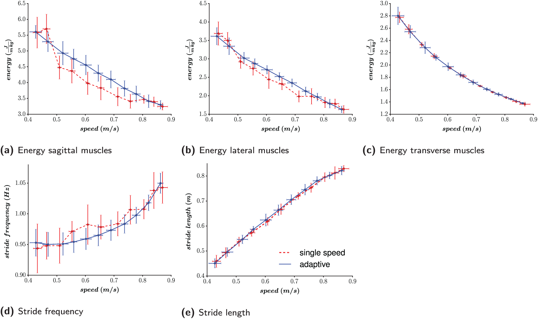
The metabolic energy consumption per unit distance for the right leg for the muscles acting in the sagittal (a), the lateral (b), and the transverse (c) planes. (d) The stride (i.e. two steps) frequency. (e) The stride length. Ten controllers are optimized with no speed adaptation (labeled single speed) for each speed reference (Experiment 1). Ten other controllers are optimized (labeled adaptive), with the ability to adapt their speed on the whole speed range (Experiment 3). For each speed, the mean and the standard deviations (each time from the ten corresponding controllers) of the different measures are pictured.

The virtual metabolic energy consumption (Figure 6a, b, and 6c) is computed for the right leg muscles, as detailed in Appendix B.3. Similar values are obtained for the left leg. As stated in Section 2.6, upper-body control is not the main focus of this contribution and barely contributes to the resulting gait. Therefore, its energy consumption is not studied.

The reported energy is actually normalized to the traveled distance. Interestingly, its value decreases with the robot forward speed. Sagittal muscles have the highest metabolic consumption, since they are the main muscles used to propel the body forward. However, the lateral muscle consumption is of the same order, due to the important efforts requested at the hip level during the stance phase. Surprisingly, transverse muscles energy consumption is also of the same order, while their only purpose was to keep the leg straight. The reason is that important gains are used for the corresponding PD controller, generating high co-contraction. A possible improvement would be to optimize these gain parameters.

Regarding the stride analysis (Figure 6d and e), an increase in the forward speed results both in an increase of stride frequency and length. This is coherent with human analysis: faster walking speeds usually correspond to faster walking frequencies and longer step lengths (Murray et al., 1966). For slow speeds, the evolution of the stride frequency is less significant than that of the stride length. This indicates that the optimizer favors stride length modulation over frequency modulation for slow speeds.

4.2. Experiment 2: speed key parameters

Following the proximo-distal hypothesis (Daley et al., 2007), speed modulation is mainly performed by the leg proximal muscles, i.e. those close to the hip. In particular, the introduction of a CPG is useful for this purpose, since it modulates the locomotion by simple control signals (Ijspeert, 2008). This section investigates which control parameters could play a significant role in forward speed modulation.

Step frequency is directly related to the CPG frequency, which can be modulated using the time constant $\tau$ . Indeed, this value is proportional to the Matsuoka oscillators period (Taga et al., 1991). As reported in Section 2.8, the CPG frequency is optimized to match the gait resulting in closed-loop frequency. Other potential parameters for speed modulation include the CPG amplitude output signals. They are controlled by the gains $k_{\mathrm{HFL}}$ , $k_{\mathrm{GLU},1}$ , $k_{\mathrm{GLU},2}$ , $k_{\mathrm{HAM},1}$ , $k_{\mathrm{HAM},2}$ , $k_{\mathrm{HAM},3}$ , and $k_{\mathrm{HAB}}$ multiplying the CPG outputs (see Appendix E.1).

Moreover, faster speeds usually involve larger torso tilt, as reported in Song and Geyer (2012). Therefore, the target torso angles ${\theta }_{\mathrm{ref}}$ (sagittal plane) and ${\mathrm{\Psi }}_{\mathrm{ref}}$ (lateral plane) are also good candidates for modulating the forward speed. Finally, the lateral swing foot placement (being controlled by the parameter ${\Lambda }_{\mathrm{ref},h}$ ) might also be dependent on the speed. Therefore, all these parameters are studied for speed modulation.

The influence of these 11 key parameters on the walking speed was analyzed as follows. An optimization was performed for a single speed of 0.65 m/s, i.e. in the middle of the target speed range of Figure 6 ( $\left[0.4;0.9\right]$ m/s). Then, all the optimized parameters were frozen, except the eleven key parameters mentioned above. The speed range was discretized with a step of 0.05 m/s. For each target speed (including 0.65 m/s again), 10 optimizations were performed, initiating the gait with the 11 key parameters corresponding to the initial speed (0.65 m/s), before switching to new ones after four steps. The evolution of these optimized parameters is reported in Figure 7 (except for the target speed of 0.4 m/s, which did not produce suitable gaits in this experiment).

Fig. 7.

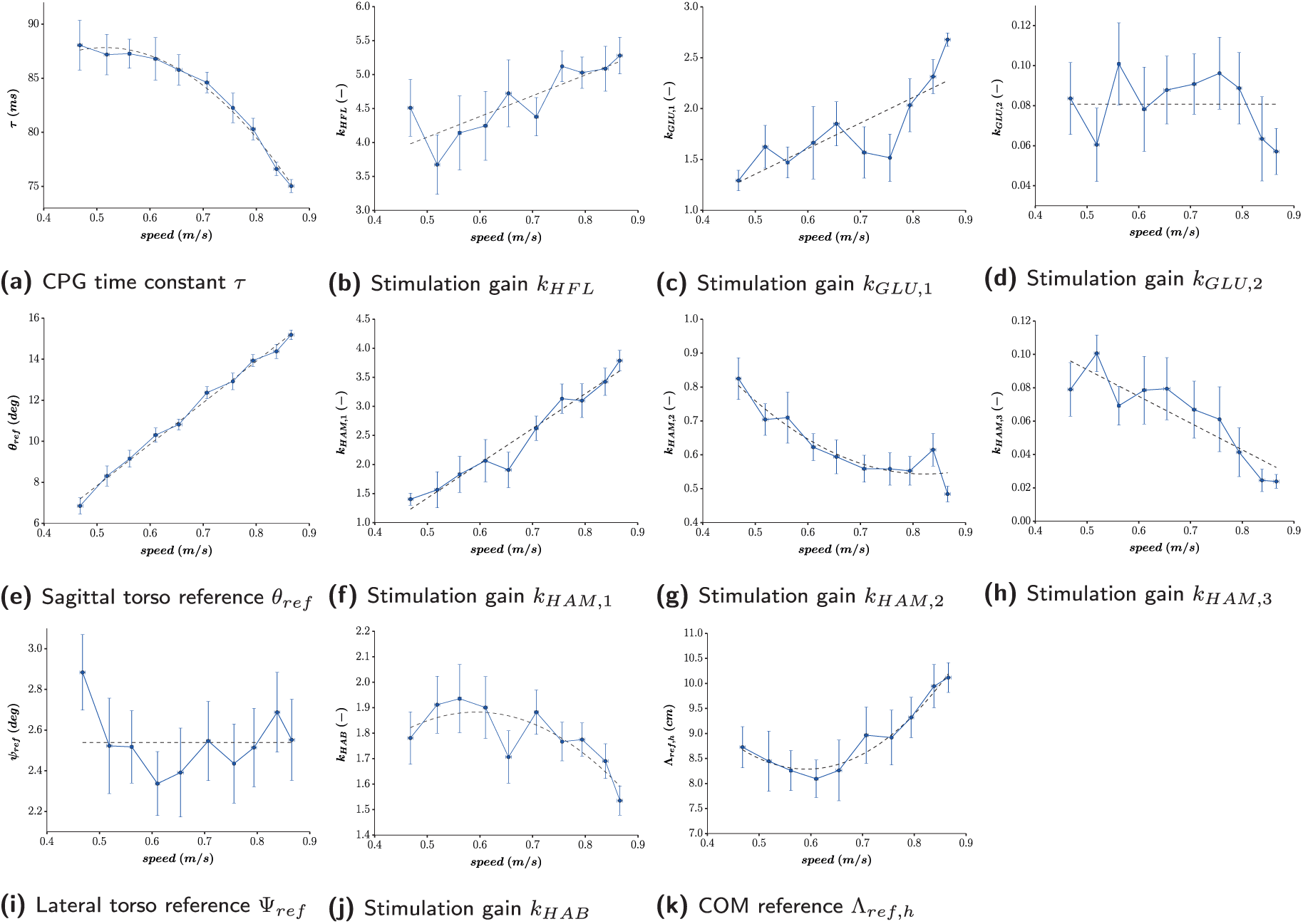
Results of Experiment 2: 10 optimizations are performed for each target speed (from 0.45 to 0.9 m/s with an interval of 0.05 m/s).The actual speed of each solution is measured, along with the optimized value of the 11 open key parameters. For each target speed, we gather the 10 optimization final results, reporting their mean and standard deviations. For graph legibility, the error bars represent half of the standard deviations. Dashed lines correspond to the polynomial approximations whose order is computed in Table 2, using the minimum mean square error method.

Intuitively, the evolution of most of these key parameters with forward speed can be approximated with polynomial functions, whose orders have to be properly selected to capture the curve without over-fitting. To do so, a model goodness-of-fit analysis using the sum of squared values of the prediction errors (Smith and Rose, 1995) was performed, as detailed in Appendix G.

Resulting p -values are presented in Table 2. The corresponding null hypothesis is that the model fits the data. Its rejection (i.e. too small p -value) indicates an overall lack of fit regarding the order selected for regression. Fixing and arbitrary threshold to 0.1, the lowest order with a p -value exceeding this threshold was selected as being appropriate for the fit. This is a less strong analysis than rejecting the opposite null hypothesis, but is considered to be sufficient to design the control rules.

Table 2.

Polynomial approximations of orders 0, 1, and 2 of the data provided in Figure 7, based on the least-squares errors. Each p-value is then computed as detailed in Appendix G. The first order with a p-value larger than 0.1 is then selected (gray cells).

	Order 0	Order 1	Order 2	Selected
$\mathbf{\tau }$	0	0.002	0.968	2
${\mathbf{k}}_{\mathrm{HFL}}$	0	0.211	0.218	1
${\mathbf{k}}_{\mathrm{GLU},1}$	0	0.002	0.015	$\varnothing$
${\mathbf{k}}_{\mathrm{GLU},2}$	0.115	0.099	0.293	0
${\mathbf{\theta }}_{\mathrm{ref}}$	0	0.463	0.649	1
${\mathbf{k}}_{\mathrm{HAM},1}$	0	0.32	0.517	1
${\mathbf{k}}_{\mathrm{HAM},2}$	0	0.022	0.169	2
${\mathbf{k}}_{\mathrm{HAM},3}$	0	0.146	0.528	1
${\mathbf{\Psi }}_{\mathrm{ref}}$	0.2	0.159	0.727	0
${\mathbf{k}}_{\mathrm{HAB}}$	0	0.028	0.162	2
${\mathbf{\Lambda }}_{\mathrm{ref},h}$	0	0.063	0.958	2

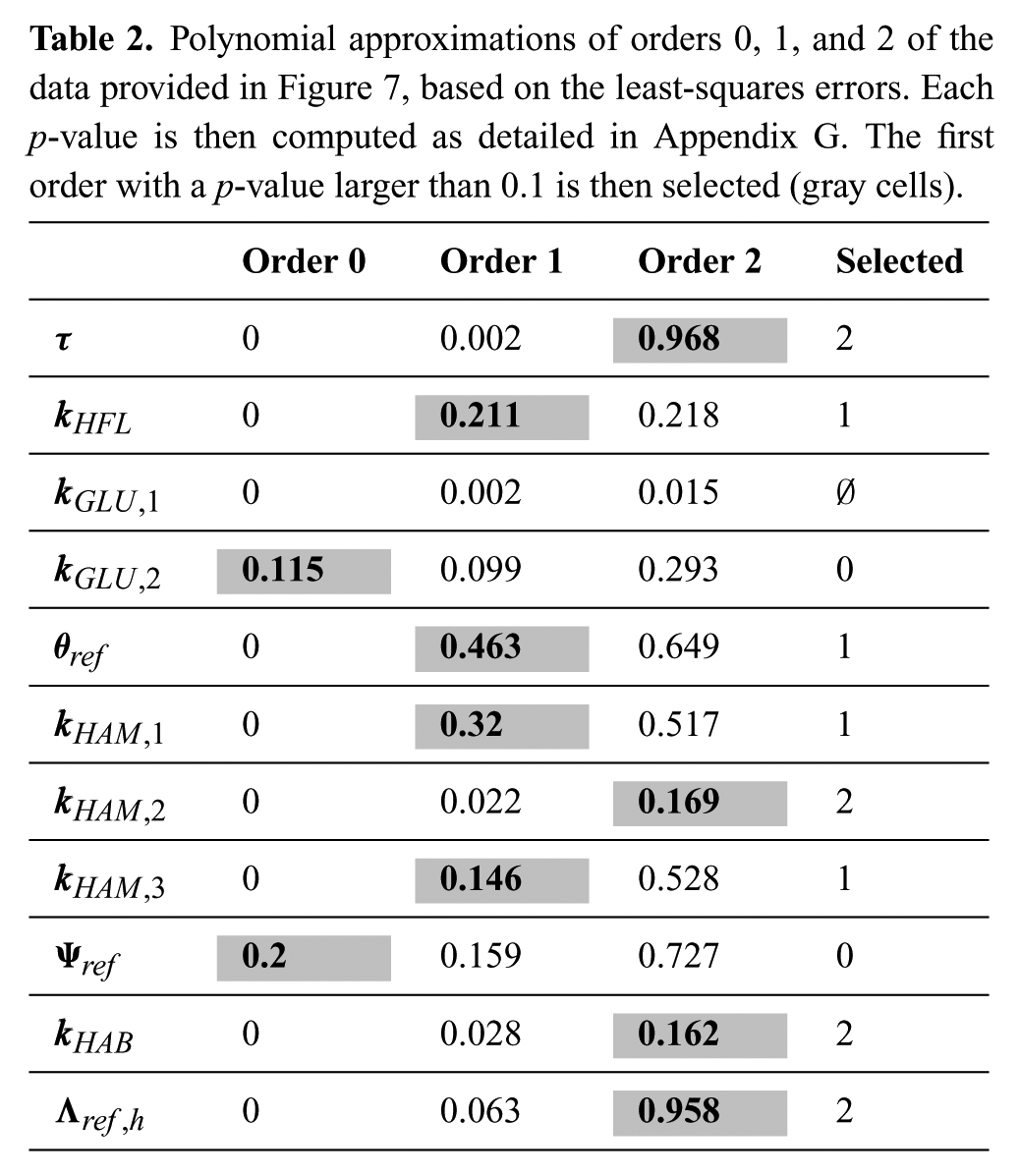
Interestingly, these results are close to those reported in Van der Noot et al. (2015b). In this earlier contribution, similar graphs were obtained when restricting the walker to stay in the 2D sagittal plane, while exploring the evolution of a subset of six of the key parameters.

As expected, the time constant $\tau$ decreases (and so the frequency increases) with higher speeds. This correlation obeys a parabolic trend, while we reported a linear one in two dimensions (Van der Noot et al., 2015b). On top of that, the corresponding frequencies are larger in three than in two dimensions, for the same speed references. This is due to the lateral balance, which is easier to maintain with shorter step durations. In addition, variations of $\tau$ are larger for higher speeds. This indicates that the optimizer favored step length modulation for slow speeds and step frequency modulation for higher speeds. This is coherent with the observations made in Experiment 1.

During the stance phase, $k_{\mathrm{GLU},1}$ and $k_{\mathrm{HAM},1}$ were both recruited to bring the torso back to its reference inclination after foot strike. This requires higher stimulations at higher speeds, due to larger inertia effects and strike impacts. This explains why these gains increase with higher speeds. Note that Table 2 reports that the polynomial fits did not reach significance for $k_{\mathrm{GLU},1}$ . Since this parameter is redundant with $k_{\mathrm{HAM},1}$ , this was considered to be not critical. For this parameter, we arbitrary chose a polynomial approximation of order 1. In the lateral plane, $k_{\mathrm{HAB}}$ is sightly larger in the middle of the speed range, indicating a stronger torso lateral stabilization for the corresponding speeds.

During the early swing phase, hip flexion increases for higher speeds. Consequently, the HFL muscles receive higher stimulations (with $k_{\mathrm{HFL}}$ increasing) while their antagonist muscles HAM receive lower stimulations (with $k_{\mathrm{HAM},2}$ decreasing). In late swing, $k_{\mathrm{GLU},2}$ and $k_{\mathrm{HAM},3}$ are used to favor leg retraction, which reduces the walking speed. This explains why $k_{\mathrm{HAM},3}$ decreases. However, no significant modulation is observed for $k_{\mathrm{GLU},2}$ , probably due to its redundancy with $k_{\mathrm{HAM},3}$ . Globally, the CPG output modulation conveys similar conclusions as those we drew in the 2D case (Van der Noot et al., 2015b).

Regarding reflexes, the torso sagittal lean angle reference ${\theta }_{\mathrm{ref}}$ increases linearly with speed, as in Van der Noot et al. (2015b). Its lateral reference ${\mathrm{\Psi }}_{\mathrm{ref}}$ , however, does not display a significant modulation, due to its high variance. Finally, the COM reference ${\Lambda }_{\mathrm{ref},h}$ driving the lateral swing hip is minimal in the middle of the speed range. This is coherent with the $k_{\mathrm{HAB}}$ evolution. Indeed, a higher $k_{\mathrm{HAB}}$ generates a higher momentum, accelerating the COM towards the swing leg (Patla et al., 1999). To counter it, the swing foot must be placed further away, inducing a smaller ${\Lambda }_{\mathrm{ref},h}$ .

4.3. Experiment 3: a single controller for the whole speed range

The controller design can now be further extended to generate any forward speed in the $\left[0.4;0.9\right]$ m/s range. The 11 key parameters studied in Experiment 2 are replaced by polynomial functions whose order is chosen according to Figure 7 and Table 2 (except for $k_{\mathrm{GLU},1}$ ). Because the modulation of $k_{\mathrm{GLU},2}$ and ${\mathrm{\Psi }}_{\mathrm{ref}}$ are actually of order 0, the corresponding parameters are constants. The speed modulation is then fully achieved with nine parameters: seven CPG parameters and two reflex parameters, as a function of the target speed (see Table 1). The four initial steps are performed with a speed reference $v_{\mathrm{ref}}$ set to 0.65 m/s, in order to achieve walk initialization. Then, $v_{\mathrm{ref}}$ can be changed to any value in the speed range, at any moment in the gait. This high-level control is depicted in Figure 1.

New optimizations were thus performed with the whole range of forward speed being embraced within a single trial. More specifically, 11 target speeds were selected (from 0.4 to 0.9 m/s with a step of 0.05 m/s). Then, the same optimization process as described in Section 2.8 was performed to find the whole parameters set (including the coefficients capturing the modulation of the nine parameters changing as polynomial functions of the forward speed). More precisely, each optimization received this whole parameter set and a range of target speeds $v_{\mathrm{ref}}$ to test (see Table 1). The resulting fitness value was computed as the average of all the fitness functions of each tested target speed. This co-optimizes all the parameters within a single optimization, leading to more efficient gaits and larger speed ranges than those presented in Figure 7.

Ten heuristic optimizations were performed using this approach. They resulted in 10 different sets of optimized parameters. The 10 corresponding optimized controllers (called adaptive controllers and capable of reaching any forward speed in the $\left[0.4;0.9\right]$ m/s range) were evaluated similarly to the so-called single speed controllers (i.e. controllers optimized for a single speed) from Experiment 1 (see Figure 6).

Since no parameter was optimized in the transverse plane, the corresponding energetic consumption was similar for the single speed controllers and the adaptive ones. In the other planes, the single speed controllers turned out to be more efficient than the adaptive ones. However, given that the adaptive controllers were optimized for a large range of speeds in a single shot and not tuned for a precise gait, this small pay-off regarding energetic cost seems a reasonable price to pay. Regarding step size analysis, the single speed controllers favor higher frequencies and shorter steps than the adaptive ones. However, these differences are rather small.

The standard deviations in Figure 6 are usually larger for the single speed controllers than for the adaptive ones. This indicates that the gaits (and underlying parameter sets) resulting from different optimizations are more similar when optimizing the whole range of forward speeds in a single trial. Globally, the sagittal energetic consumption and the step frequency display the highest deviations (relative to their respective ranges) between different optimizations. However, the global evolution of all these features with the speed remains close between the different optimization runs. Thus, while in principle there could have been multiple local minima in the search space, the optimizations tended to converge to similar optimal parameter sets and resulting gaits.

4.4. Experiment 4: forward speed modulation

Among the adaptive controllers of Experiment 3, we select one of them and refer to it as the reference controller. In the rest of this contribution, we only report results that were obtained with this controller (i.e. corresponding to the same set of optimized parameters in the whole paper). This controller is available in Extension 1.

The forward speed of the robot can be controlled on-line by adapting the speed reference $v_{\mathrm{ref}}$ . The speed modulation achieved with the reference controller on COMAN is visible in Extension 2 and in Figure 8.

Fig. 8.

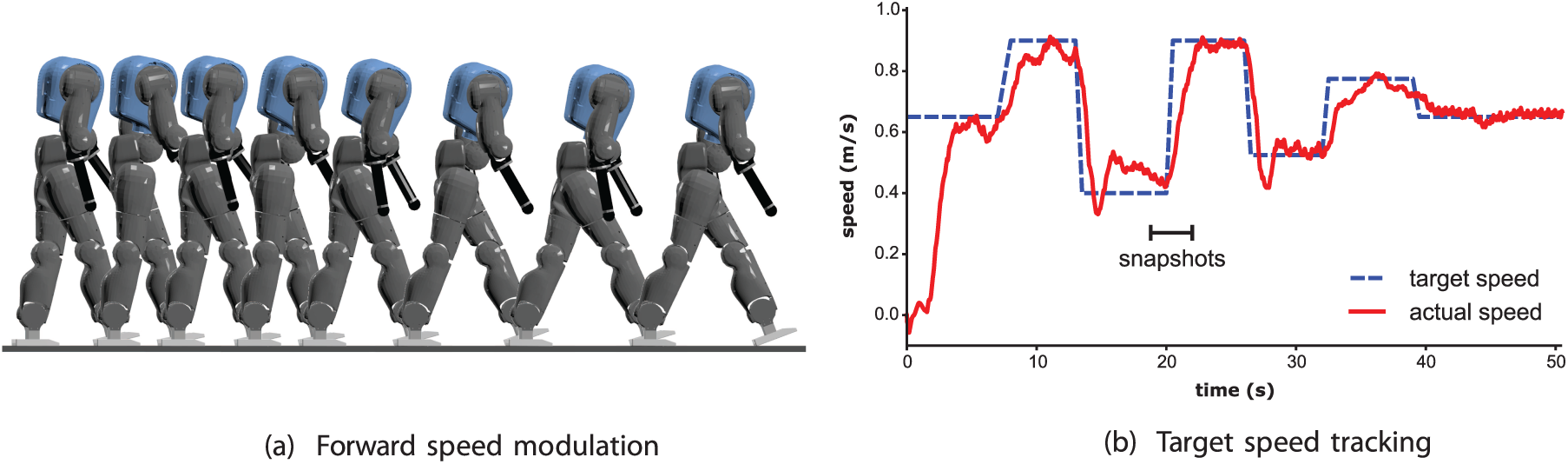
(a) Snapshots of an experiment where the robot forward speed is modulated. (b) Tracking of the target speed $v_{\mathrm{ref}}$ (dashed line), where the robot actual forward speed (solid line) is post-processed with a running average of 1 s. The time interval during which the snapshots of (a) are taken is also displayed. A video of the corresponding experiment is provided in Extension 2.

In this experiment, the target speed is modulated in the full range, i.e. from 0.4 to 0.9 m/s. The resulting speed (post-processed with a running average of 1 s) can follow this reference with accelerations up to $\pm 0.25$ m/s². This represents less than two strides to go from one speed extremum to the other.

5. Comparisons with an inverted pendulum controller and with human data

The gait obtained from this neuromuscular controller can be compared with both human data and to gaits resulting from more traditional controllers, typically using inverse kinematics or dynamics transformations to compute position or torque references at the joint level (Fitzpatrick et al., 2016). Therefore, the gait of our reference controller is compared with that resulting from a more traditional LIP controller and to human data. These comparisons are performed on kinematics and dynamics data in steady state. Correlations between our muscles activations and surface electromyography signals (EMG) extracted from human data are also reported. Finally, comparisons to the LIP-based controller are further extended by analyzing the energetic consumption.

5.1. Experiment 5: steady-state gaits comparisons

Among the controllers relying on inverse modeling, we selected that reported in Faraji et al. (2014b). In that paper, a LIP-based torque controller could achieve gait modulation on the simulated COMAN. Using the same embodiment as ours offers to make direct comparisons with our own results (labeled neuromuscular). Importantly, this LIP-based controller generates slower gaits than those obtained with our neuromuscular model. Therefore, these comparisons are not ideal but remain valuable to providing a benchmark comparing our controller with more traditional approaches.

To compare these results with human measurements, we use the data from Bovi et al. (2011). In that contribution, measures were performed on 20 adult subjects. This includes the temporal evolution of joint positions, torques, ground contact forces, and EMG signals. We selected the data set with subjects walking at their natural (i.e. unconstrained) speed.

The average speed of the 20 adult subjects in Bovi et al. (2011) was equal to $71.36\mathrm{\%BH}$ /s, where BH stands for body height. Considering that COMAN height would be close to 1.06 m if it had a head, this corresponds to a speed of 0.75 m/s. Therefore, data for the neuromuscular controller was extracted from our reference controller walking with this reference speed. The LIP-based controller of Faraji et al. (2014b) is not capable of reaching such a high speed. Consequently, the data presented from its resulting gait were obtained when walking close to its maximal speed, i.e. 0.31 m/s. It should also be noted that the LIP-based controller does not include a model of the electrical actuators, therefore bypassing the noise component introduced in Section 3.2. The following sections report different measurements performed on this experiment.

5.2. Kinematics and dynamics

The position and torque profiles extracted from Experiment 5 are displayed in Figure 9, where the data obtained with COMAN (i.e. the LIP and neuromuscular controllers) were averaged over 20 consecutive gait cycles (right leg). We computed the cross-correlation coefficient between each controller gait and the human data shifted in time. More precisely, we tested 100 time shifts equally spaced between $0\%$ and $100\%$ of the gait cycle. Here, we report the maximum of these cross-correlation coefficients, namely R and the corresponding time shifts $\mathrm{\Delta }$ as a percentage of stride (Wren et al., 2006).

Fig. 9.

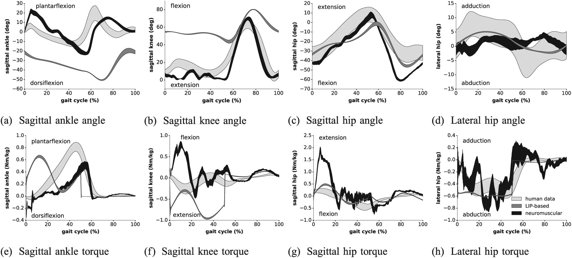
Kinematic and dynamic profiles of Experiment 5: the human data from Bovi et al. (2011) (natural speed) is compared with our neuromuscular controller (0.75 m/s) and with the LIP-based controller (0.31 m/s) from Faraji et al. (2014b). The averages of the different measures are displayed over one gait cycle (starting at right foot strike), augmented by their standard deviations (shaded areas).

The sagittal joint kinematics globally shows good matching for the neuromuscular model (ankle: $R=0.8,\mathrm{\Delta }=-9\%$ ; knee: $R=0.95,\mathrm{\Delta }=0\%$ ; sagittal hip: $R=0.97,\mathrm{\Delta }=0\%$ ), although this is lower for the ankle than the hip and knee. This might be due to the rigid foot used on our model, different from the human one. Indeed, in Colasanto et al. (2015), replacing the robot rigid foot by a model of a human prosthesis led to more robust gaits. This is a possible future improvement for our experiments. The lateral hip kinematics corresponds to a low correlation ( $R=0.57,\mathrm{\Delta }=-35\%$ ). However, the corresponding human motion is rather small and displays a large variance. Therefore, this low correlation is more difficult to interpret.

The correlations obtained with the LIP-based controller are systematically lower than with the neuromuscular controller, in the sagittal plane (ankle: $R=0.32,\mathrm{\Delta }=-40\%$ ; knee: $R=0.87,\mathrm{\Delta }=-6\%$ ; hip: $R=0.93,\mathrm{\Delta }=0\%$ ) and significantly better in the lateral plane (hip: $R=0.93,\mathrm{\Delta }=-5\%$ ). In particular, there is a large offset in the sagittal ankle and knee angles. This behavior (bent knee walking) is typical of most humanoid gaits. The main reason is usually related to the deterioration of their controllers in configurations involving a singularity (Kurazume et al., 2005).

Interesting observations can also be reported from the torque cross-correlations. For the neuromuscular controller, the matching is good for the sagittal ankle and lateral hip joints, but not for the two other joints (ankle: $R=0.92,\mathrm{\Delta }=-5\%$ ; knee: $R=0.24,\mathrm{\Delta }=82\%$ ; sagittal hip: $R=0.53,\mathrm{\Delta }=-3\%$ ; lateral hip: $R=0.89,\mathrm{\Delta }=5\%$ ). The ankle plantar flexion is also of smaller magnitude. As mentioned previously, this might also be due to the lack of compliance in the foot being simulated.

The lower correlations for sagittal knee and hip are also observed in Geyer and Herr (2010). Human knee torque mainly oscillates around the zero axis during the stance phase. This is also the case in our model, although this oscillation is similar in anti-phase. In Figure 9b, a small knee flexion is observed after strike, only for human data. To prevent from collapsing, humans thus apply an initial extension torque. In our model, the opposite happens: heel strike is followed by a slight knee over-extension, counteracted by a flexion torque. Regarding the sagittal hip, the main difference is the larger extension torque after strike, to prevent the torso from collapsing. However, it should be noted that other contributions reported human data displaying a similar large extension torque (Riener et al., 2002; Zelik and Kuo, 2010). This is likely highly dependent on the location of the hip center of rotation, which might also explain our own results. Yet, these bumps usually do not exceed 0.8 Nm/kg, indicating that our first hip reaction is above any human data.

The LIP-based controller torques show similar correlations with human data, except for the sagittal ankle (ankle: $R=0.89,\mathrm{\Delta }=29\%$ ; knee: $R=0.71,\mathrm{\Delta }=-19\%$ ; sagittal hip: $R=0.66,\mathrm{\Delta }=-1\%$ ; lateral hip: $R=0.98,\mathrm{\Delta }=5\%$ ). The ankle torque in the sagittal plane shows a large phase shift regarding the peak in the stance phase. This is due to the lack of heel–toe motion and toe push-off. The lower variances can be explained by the lack of modeling of the motor dynamics and simulation noise.

Figure 10 shows the vertical GRFs measured during the same experiments. In particular, human data displays an M-shaped pattern, i.e. a well-known feature of human walking gaits. In contrast, the LIP-based controller exhibits a nearly flat profile during its stance phase, and initiates its swing phase earlier. In contrast, the neuromuscular controller stance phase is better aligned with human data and displays oscillations in the GRF amplitude. However, the corresponding pattern differs from the human one. This discrepancy is probably due to the use of rigid feet in our experiment (and so to the lack of damping at strike impact), in contrast to human feet. Other possible reasons include the lack of toes, the foot length being shorter than the human one, and the knee over-extension issue mentioned previously.

Fig. 10.

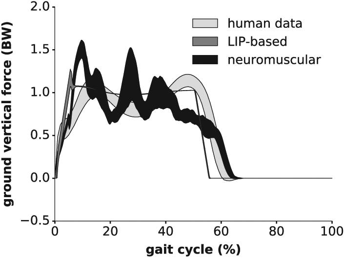
Vertical GRF profiles of Experiment 5 (right leg), normalized to the body weight (BW). Both the LIP-based and neuromuscular data are post-processed with a running average of 50 ms.

5.3. Muscle activations

Similarly to Geyer and Herr (2010), activations controlling the virtual muscles (neuromuscular controller) can be compared with real human EMG signals. Figure 11 reports this comparison for the following muscles: (a, b) soleus, (c, d) tibialis anterior, (e, f) gastrocnemius medialis, (g, h) vastus medialis, and (i, j) gluteus maximus.

Fig. 11.

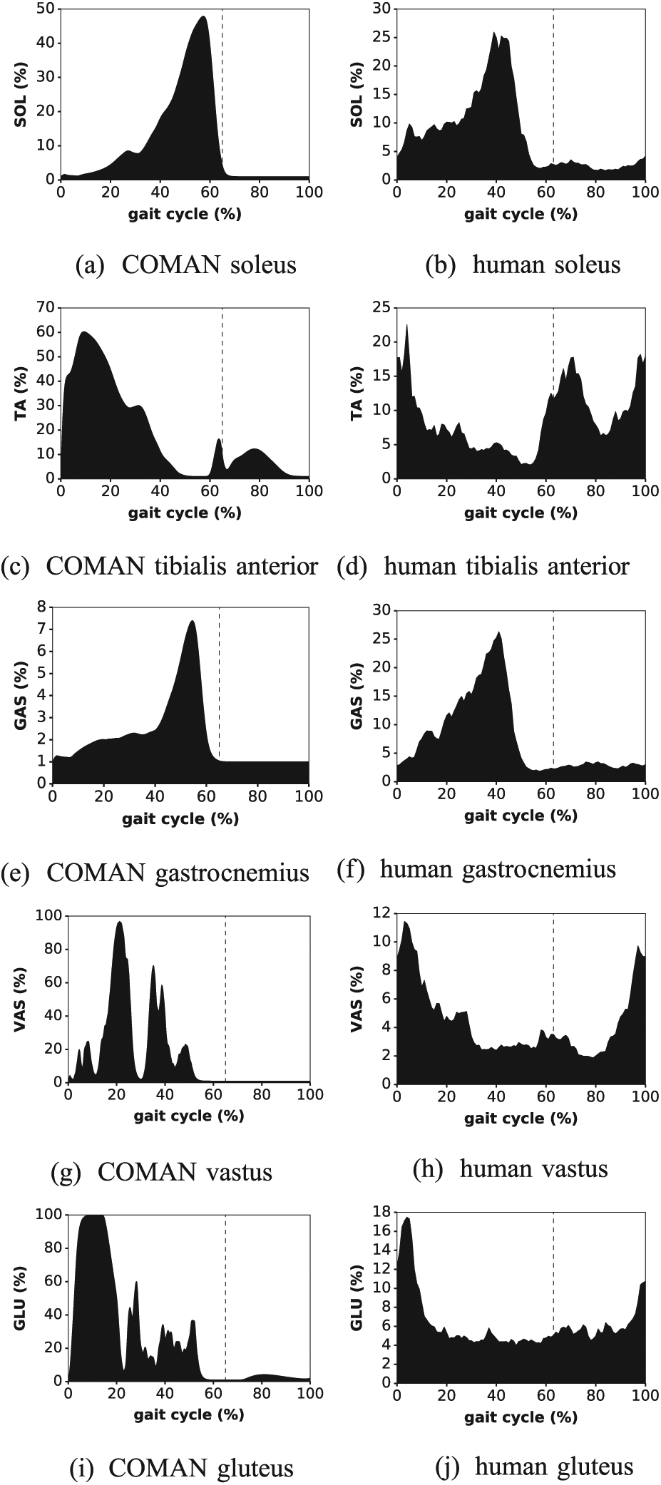
Muscle activation profiles of Experiment 5: the activations obtained with COMAN (neuromuscular controller) are compared with EMGs measured on walking humans (Bovi et al., 2011). Owing to the high variances of these signals, only their average is reported. The dashed line reports the transition from stance to swing.

The $\mathrm{SOL}$ and GAS muscle groups feature high cross-correlations coefficients, although with a significant phase shift (SOL: $R=0.96,\mathrm{\Delta }=-14\%$ ; GAS: $R=0.96,\mathrm{\Delta }=-13\%$ ). This shift corresponds to the one of Figure 9 for the joint being controlled by these two muscles, namely the sagittal ankle. Once again, this might be related to the lack of compliance in the foot, affecting the push-off phase. Correlations for the other muscles are typically lower (TA: $R=0.69,\mathrm{\Delta }=58\%$ ; VAS: $R=0.7,\mathrm{\Delta }=-15\%$ ; GLU: $R=0.76,\mathrm{\Delta }=-3\%$ ). The stance activations are usually displaying a reasonable matching. During swing, however, our virtual muscles are nearly silent because the legs rely on ballistic motion. This is not the case in the reported human measurements.

5.4. Energetic consumption

In order to compare the energetic consumption of the neuromuscular controller with the LIP-based one, the square of the joint torques are integrated over one gait cycle. Figure 12a reports the different joint contributions for the right leg (the left leg results are identical). As indicated in Section 2.6, the upper-body motion barely contributes to the gait and is therefore not included in this analysis. In contrast to the previous analyses, the measurements were performed with the neuromuscular controller over its whole range of forward speeds. The gaits resulting from the neuromuscular controller are compared to the highest speed (0.31 m/s) obtained with the LIP-based controller (i.e. same gait as in Figure 9).

Fig. 12.

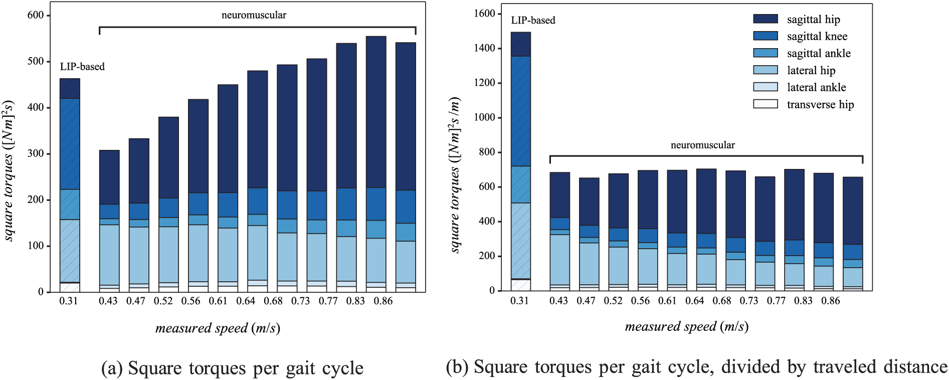
Estimate of the energetic consumption of both controllers tested in Experiment 5. (a) The sum of square of the joint torques for the LIP-based controller (hatched) and the neuromuscular one (non-hatched), both integrated over one gait cycle, i.e. one stride. The measures were performed on the right leg at different speeds, and averaged over 20 gait cycles. The contributions of each joint correspond to different colors (see legend). (b) The same result, normalized by the distance traveled during one gait cycle.

Globally, the neuromuscular controller displays lower torque profiles than the LIP-based one, when walking slower than 0.64 m/s. As expected, the LIP-based controller recruits large torques at the knee level, due to the fact that this joint stays bent during the whole stance phase. The neuromuscular model, however, recruits smaller knee torques, but requires much higher torques at the sagittal hip joint (increasing with speed). This is coherent with the observations reported in Figure 9.

Torques produced by the ankle in the sagittal plane are also far less important with the neuromuscular controller, especially at slow speeds. The hip torque in the lateral plane are larger with the LIP-based model. Finally, the remaining joints torques are negligible. In particular, the high virtual metabolic energy consumption of the transverse hip (see Figure 6c) does not translate in higher torques.

However, this analysis did not take the traveled distance into account. In Figure 12b, the same results are displayed, with a normalization by the stride length. Interestingly, the total square torque for the neuromuscular model is quite constant as a function of the forward speed. In particular, the increase in the sagittal hip torque is compensated by the extra traveled distance. This analysis strongly penalized the LIP-based controller since its normalized sum of square torques is about more than twice larger than that of the neuromuscular controller.

6. Gait robustness

The following section reports experiments with the robot walking blindly (i.e. with no perception of its environment), using the reference controller. Its robustness was tested against external pushes, stairs, slopes, and irregular ground (on top of the simulator noise). During all these experiments, no parameter modulation was applied to the controller.

6.1. Experiment 6: resisting pushes

First, the following experiment was performed. COMAN received random pushes on the torso when walking at different speeds. These pushes were applied with a magnitude between 0 and 30 N during 0.2 s in the transverse plane. Ten pushes were applied with a time interval randomly selected between 5 and 6 s. Each push orientation in the transverse plane was randomly selected in the $]-\pi ;\pi ]$ interval (i.e. all possible directions selected with an equal probability). Robustness was quantified by counting the number of pushes the robot could sustain without falling.

This result is reported in Figure 13a, for the $\left[0.4;0.9\right]$ m/s speed reference range (with a discretization of 0.05 m/s). Globally, higher speeds can resist higher pushes. The only exception is the maximal speed (i.e. reference of 0.9 m/s), which was less stable. Indeed, less-stable gaits were usually obtained for the extrema of the tested speed range.

Fig. 13.

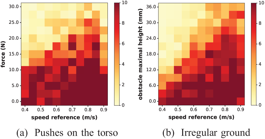
For the whole spectrum of speed references, COMAN faced two kinds of external disturbances. In (a), pushes were applied on its torso (Experiment 6). The color map represents the number of pushes the robot resisted (averaged over five runs) before falling, as a function of the push amplitude. In (b), COMAN was walking on the irregular ground displayed in Figure 17 (Experiment 9). The values of the corresponding $H_i$ heights were randomly selected in the range whose maximum value is reported on the vertical axis. The color map represents the forward distance (i.e. along the x axis (in meters)) COMAN walked before falling (limited to 10 m and averaged over five runs).

Another illustration of the robot resistance to external pushes is provided in Extension 3. In this experiment, COMAN walked with the reference controller at a speed of 0.65 m/s. During walking, 10 balls with a density of 750 kg/m³ were thrown to it. In particular, after absorbing a ball push, the walker can recover its previous gait, thanks to the CPG entrainment (Ijspeert, 2008).

6.2. Experiments 7 and 8: natural adaptation to stairs and slopes

Experiment 7 established the capacity of the robot to adapt to ascending and descending (small) stairs. This is presented in Extension 4, with the reference controller walking with a speed reference of $0.85m∕s$ . Snapshots of this experiment are displayed in Figure 14. The corresponding stair is made of five ascending and five descending steps, each with a width of 50 cm and a height of 2 cm. This performance is similar to that of Geyer and Herr (2010), pending a scaling to our robot size. Interestingly, our controller can even adapt when its foot lands between two consecutive stair steps, as can be seen in Figure 14.

Fig. 14.

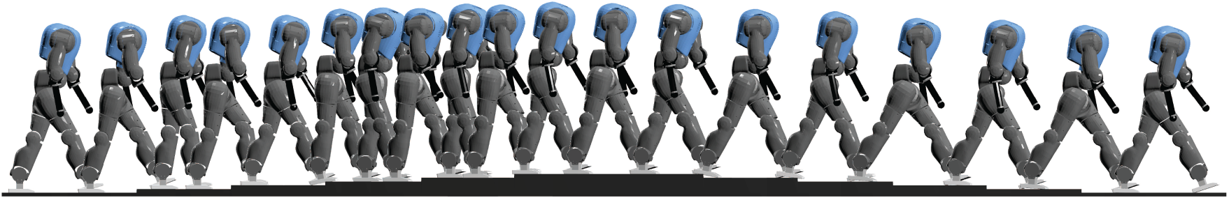
Snapshots from Experiment 7: COMAN walked blindly on an ascending and descending stair. Step length was automatically adapted to the environment, without changing the controller. At the end of the stair, COMAN retrieved its initial gait, thanks to the CPG. Extension 4 reports the whole experiment.

Similarly, Experiment 8 tested the robot ability to adapt to ascending and descending slopes. In Extension 5, COMAN walks blindly with a speed reference of 0.85 m/s on a flat ground before facing a rising slope of $2.58^{\circ }$ . Snapshots of this experiment are provided in Figure 15.

Fig. 15.

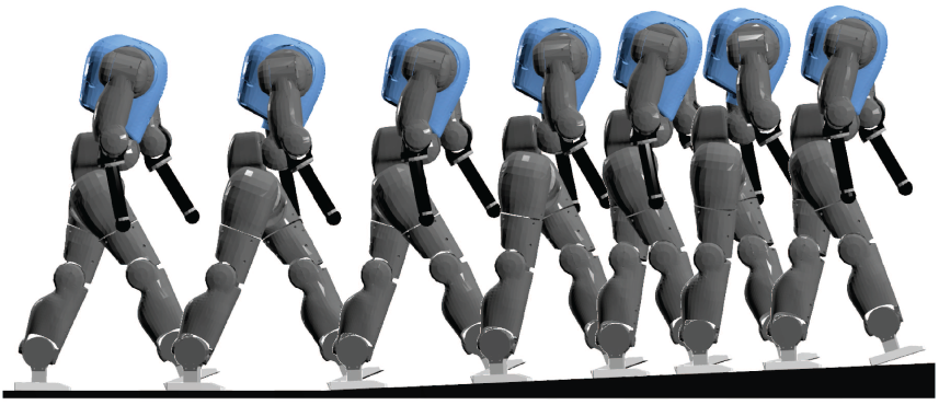
Snapshots of Experiment 8, where the robot faced a slope (here, $2.58^{\circ }$ ). It automatically adapted its step length, with no change in the controller. Extension 5 reports the whole experiment.

Similar results were obtained on the whole speed range, as reported in Figure 16. There is no global trend for descending slopes. In general, COMAN can walk on negative slopes with an angle smaller than $-2.29^{\circ }$ ( $-4\%$ ). For rising slopes, a clear correlation appears with the forward speed. As can be seen in Figure 15, the walker naturally decreases its step length (and so its speed) when climbing a positive slope. Therefore, a higher initial speed can withstand larger slopes. With its maximal speed reference, COMAN can climb slopes up to an angle of $2.58^{\circ }$ ( $4.5\%$ ). This is similar to the results reported in Geyer and Herr (2010).

Fig. 16.

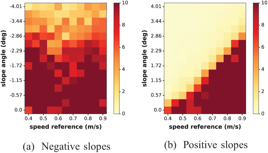
Results from Experiment 8: for the whole spectrum of speed references, COMAN faced ground with slopes of different angles (from $0^{\circ }$ to $4^{\circ }$ with a discretization of $0.29^{\circ }$ , for positive and negative angles). The color map represents the distance traveled on the slope (in meters) before a possible fall (limited to 10 m and averaged over five runs).

6.3. Experiment 9: natural adaptation to irregular grounds

In Experiments 7 and 8, the walker robustness was tested when facing uneven ground with regular patterns (i.e. stairs and slopes). This experiment quantifies its robustness to irregular grounds. The description of the corresponding ground is presented in Figure 17. Different grounds can then be tested with randomly selected heights $H_i$ .

Fig. 17.

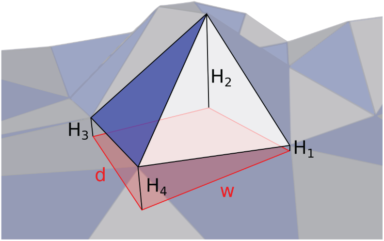
Description of the irregular uneven ground generated for Experiment 9. Each triangle composing the ground mesh is based on a rectangle of size $d\times w$ with four randomly selected heights $H_i$ at its corners ( $d=w=50$ cm).

In Extension 6, COMAN walks on this ground (with a speed reference of 0.65 m/s), where the $H_i$ heights were randomly selected in a range of $\left[0;25\right]$ mm. Figure 13b reports the result of this experiment over the whole speed reference range and for different maximum obstacle heights. Similarly to the results of Experiment 6, higher speeds produced more robust gaits, except for the maximum speed (0.9 m/s), intrinsically less stable.

7. Discussion

The work presented here offers an alternative locomotion controller for humanoid robots. The controller can generate gaits across a range of speeds close to the normal human walking one, by recruiting virtual muscles controlled by CPG and reflex signals. By embracing the concept of limit cycle walking, it relaxes constraints inherent to more traditional locomotion controllers. In particular, singularity configurations such as stretched legs can be reached, generating faster and more energetically efficient gaits.

7.1. Interest of the bio-inspired approach

While using (virtual) muscles might seem natural when working on real human models or on animation characters, it is less obvious for humanoid robots equipped with electrical actuators. This paper showed that using muscles as an intermediate layer offers several interesting properties: (i) the virtual muscles generate continuous torques, being smooth to track for the low-level torque controller; (ii) human-like gaits can be obtained by minimizing the metabolic consumption of these virtual muscles (see Section 2.8), in a way likely similar to what humans do; (iii) this configuration, being similar to that of a human, provides the ideal framework for comparing ourmodel with human data, including the level of muscle activations; and (iv) the walker benefits from the viscoelastic muscle properties, i.e. human-like joint impedance. Regarding this last point, the exact effects of the muscular viscoelastic properties still need to be quantified, which is a potential topic for follow-up work. Finally, note that minimizing the metabolic consumption of virtual muscles (point (ii)) is not a priori equivalent to minimizing the robot’s electrical energy consumption. However, the same optimization tool could be used to minimize this electrical energy consumption (i.e. maximizing the actuators efficiency) by replacing the metabolic energy measure by the electrical consumption of the motors. Future work will explore the influence of this regarding the gait kinematics and robustness.

Experiment 5 further showed that it was possible to drastically reduce the joint torque contributions with the proposed method, in comparison with more traditional controllers. This could potentially lead to important energetic cost reductions during locomotion. However, this was tested on two very different speed ranges. More specifically, the highest speed of the LIP-based controller of Faraji et al. (2014b) was close to the lowest one of our neuromuscular controller. Therefore, an alternative approach would be to use both of these controllers on the same robotic platform, pending the implementation of a transition mechanism as a function of the forward speed. In particular, the neuromuscular controller is likely more appropriate to quickly and efficiently reach a desired spot. A controller recruiting foot step planning would in contrast be more appropriate when accurate positioning is requested. Alternatively, the proposed neuromuscular controller could also be extended to generate slower walking speeds.

Last, but not least, this approach is also advantageous regarding computational cost. A single iteration of our neuromuscular controller (i.e. CPG + reflexes + virtual muscles) requested an average time of 61 $\mu$ s to be computed (on the same computer as that reported in Section 3.2). This is more than 16 times faster than the COMAN controller sampling rate, namely 1 ms. In contrast, many existing locomotion controllers use demanding computations of inverse kinematics and/or dynamics. This often leads to critical issues to fulfill the real-time constraints.

7.2. Robustness to unperceived environments

Gait robustness is one of the major issues preventing robots from being used in unknown environments. In particular, many biped locomotion controllers require an accurate dynamic model of the robot, resulting in poor robustness when there are errors in this model. Other approaches, such as the virtual model control proposed in Pratt et al. (2001) require however no dynamic model of the robot to achieve robust gaits during blind walking.

Here, the blind walking experiments performed on the COMAN platform demonstrated impressive robustness when walking in perturbed environments. In particular, the viscoelastic muscle properties commanded by the combined action of the CPG and the reflexes could automatically adapt the gait to various perturbed environments. Importantly, this was achieved without changing a single parameter of the controller. A perfect knowledge of the environment was therefore not requested, which is a key advantage in order to bring humanoid robots in our natural day-to-day life. Using the CPG as a central element, the robot could return to its normal gait after perturbation. This was particularly outlined in Experiments 6–9.

The controller could be further extended to detect possible falls and trigger additional reaction primitives. In Li et al. (2015), an energy-based fall prediction method is presented for this purpose. Similar strategies could likely allow the walker to withstand higher perturbations than those performed in the blind walking experiments.

7.3. Gait modulation

Motion diversity control (e.g. deliberate obstacle avoidance) might be easier to achieve with more traditional methods relying on inverse kinematics or inverse dynamics. However, similar motion diversity can also be found when using neuromuscular models. For instance, Desai and Geyer (2013) revisited the model of Geyer and Herr (2010) in order to control the swing leg placement. This model was further extended in Song and Geyer (2015) to avoid obstacles by increasing the foot ground clearance or the step size. Similar performances can also be obtained with CPG modulations, as we reported in Van der Noot et al. (2015b), with the objective of stepping over a hole.

In this contribution, we showed that the inclusion of a CPG could modulate the forward speed by adapting nine key control parameters as linear or quadratic functions of the target speed. This resulted in high-speed variations, over a range close to the normal human one, when scaled to the robot size. Because both the step frequency and length are adapted, it provides full control of the foot step placement, in order to avoid small obstacles. However, a high-level controller (see Figure 1) modulating the CPG inputs to generate desired gait alterations was not explored and is a potential avenue for future developments.

7.4. Parallels with human locomotion

Experiment 5 showed that this controller could also be used to investigate models of human locomotion. This was examined through comparisons with human kinematics and dynamics measurements, as well as EMG signals. Our controller recruited Hill-type muscle models commanded by reflexes, and Matsuoka oscillators, which are components developed on a solid biological background. Our CPG network was divided into two parts: the “rhythm generator” neurons and the “pattern formations” ones. Using a similar two-level CPG biological architecture, McCrea and Rybak (2008) reproduced results observed in experiments of fictive locomotion with decerebrated cats. Our approach also followed the proximo-distal hypothesis that was verified by Daley et al. (2007) on avian bipeds. In other words, muscles close to the hip mainly received feed-forward signals (i.e. from the CPG) while the distal muscles (being highly load-sensitive) received feedback activations (i.e. reflexes).

Using this structure, the modulations of the CPG frequency and amplitude, together with two reflex parameters, led to large forward speed variations and step modulation, as shown in Experiments 3 and 4. Thus, similarly to the work performed by Taga (1994), Paul et al. (2005), or Rossignol et al. (2006), this contribution also supports the assumption that CPGs could play a major role in human locomotion, at least for gait modulation.

Importantly, the recruitment of CPGs to control the walking of most vertebrates is widely accepted, but the neural circuitry generating human locomotion is still not entirely unveiled (Dzeladini et al., 2014; Minassian et al., 2017). The work of Geyer and Herr (2010), further extended in Song and Geyer (2015), obtained similar results as ours, although they implemented only reflex pathways (i.e. without CPG). Therefore, the recruitment of CPG networks during human locomotion remains a matter open to debate.

While many studies use a deductive approach to understand human locomotion (Lacquaniti et al., 2012), this contribution offers a synthesis approach to test hypotheses on human walking. In particular, this is potentially valuable to provide insights about neural and orthopedic disabilities, by understanding their effects on walking, and thus possibly contributing to develop new treatments. Yet, it is important to note that the musculoskeletal model developed here is a high-level approximation of control principles found in human motor control, not an accurate computational neuroscience model.

Divergence with real human data could possibly lead to model refinements, with the purpose to better explain human locomotion mechanisms. For instance, the large torque peak experienced by the sagittal hip after foot strike could be reduced by the introduction of a stance preparation phase. Indeed, this lack of preparation resulted in an insufficiently damped impact and thus in a large forward torso tilt, as explained in Geyer and Herr (2010).

Non-sagittal leg control could also be improved by taking inspiration from human strategies. For example, humans use the hip internal rotation, even in straight walking. This advances the swing leg and increases the step length (Stokes et al., 1989). A possible improvement of our controller would be to integrate this mechanism. In addition, the hip lateral position could sometimes bring the swing leg too close to the stance one, resulting in possible collisions between the legs. In our experiments, this was sometimes observed at speed extrema and during perturbed walking. A first naive solution would be to increase the weight of the fitness stage favoring large lateral distances between both feet. However, this might reduce the range of achievable speeds. Another solution would be to increment the lateral hip swing control. Yet, this depends on the walker embodiment being used.

Muscles coordination during human locomotion is a complex task due to the large redundancy in the musculoskeletal system (Ting et al., 2012). To solve this over-actuation problem, human motion control possibly relies on muscle synergies, i.e. on the covariation of muscle activities. Synergies virtually decrease the number of degrees of freedom (Aoi et al., 2010). In our work, muscle synergies are captured by two factors. First, the number of muscle groups (mainly inspired from Geyer and Herr, 2010) is much smaller than the actual number of human muscles. Second, some synergies are generated by our reflexes and CPG signals. For instance, the combined activation of the HAM and GLU muscles in early stance stabilizes the torso. Yet, other synergies could be explored, in particular if more muscles were added to the musculoskeletal system.

The controller could also be tested on a model closer to the human morphology than COMAN. For instance, the human femoral joint is quite different from the robot hip joints. Similarly, feet closer to the human ones could by used on the robot. In Colasanto et al. (2015), replacing the rigid feet of COMAN by compliant prostheses led to more robust gaits, when using similar neuromuscular control rules.

Computer graphics animation is another avenue for the development of such models, for example through the generation of motion and torque patterns incorporating biomechanical constraints (Wang et al., 2012). Similar neuromuscular models are not limited to humans but could possibly be extended to many biped creatures, as demonstrated by Geijtenbeek et al. (2013) on an ostrich model.

7.5. Perspectives

A natural extension of the forward speed modulation approach reported in this paper would be a module governing steering actions, i.e. changes in the heading direction. This would make possible to modulate both the heading direction and the radius of curvature of the biped walker trajectory, and thus to reach any point in a 3D environment and to navigate around obstacles.

As detailed in Section 7.4, the controller is valuable to better understanding human locomotion and to investigating possible pathologies. However, significant differences with human data were reported. These divergences could be more thoroughly investigated to obtain gaits closer to human ones. This could be done by refining the musculoskeletal model and the neural controller rules, but also by using a model (instead of a robot) close to the real human morphology (e.g. with toes and some compliance in the segments).

Interestingly, the bio-inspired approach developed here could also be applied to different body types, and even to extinct species. For instance, computer simulations and biomechanical modeling are considered as some of the most rigorous methods to reverse-engineer the gait of dinosaurs. By combining solid evidence such as the morphology of their limb skeletons with external and muscular forces, it is thus possible to reconstruct physically plausible motions (Hutchinson and Gatesy, 2006). Therefore, neuromuscular controllers could possibly be adapted to theropod (i.e. bipedal dinosaurs, such as Tyrannosaurus) gaits.

All the tests performed in this contribution used a faithful simulation model of the COMAN platform (including its actuator dynamics and noisy torque sensing). Therefore, the controller has the potential to be tested on a real robotic device. Similarly to Van der Noot et al. (2015a), this transfer would require some care regarding the dynamic non-idealities (e.g. impact, friction, and backlash).

There is increasing interest in bringing humanoid robots out of the laboratories, as emphasized during the recent DARPA Robotics Challenge. However, biped locomotion remains an important challenge, as illustrated during the terrain task of this contest. Indeed, during the corresponding trials, only 2 of the 16 teams successfully completed the entire terrain task without requiring an intervention, so that the walking challenge for the finals had to be simplified (Johnson et al., 2016). The present contribution does not target DRC-like tasks, but rather studies the scientific question of exploring the benefits of human-like musculoskeletal systems, together with their control properties. This is scientifically interesting, but also potentially valuable for robotics locomotion since humans are still much better than humanoid robots at tackling complex terrains. Moreover, the leg stretching obtained using our approach would potentially offer to cross larger obstacles and to climb stairs with higher steps, in comparison with walkers displaying continuous knee bending.

While bipedal robots are currently far from the walking capabilities of real humans in terms of robustness and energy efficiency, this contribution thus shows that neuromuscular controllers hold the potential to make a step towards this achievement. Indeed, the generated gaits are closer to the human ones, and so, more adapted to our surroundings. In the future, robots might be able to adapt to our environment, rather than us having to adapt our environment to the robot limited skills.