
Abstract
In this paper, the modeling of a redundant SCARA-type manipulator robot with five degrees of freedom is presented. We propose three controllers - hyperbolic sine-cosine, sliding mode, and calculated torque - which are applied to the discussed model. A simulation environment is developed using MatLab/Simulink programming tools. This simulation environment is employed to perform several tests (including actuators' dynamics) on the model of the redundant manipulator, with each different controller, under path tracking requirements. Results were obtained from comparative curves and rms index for joints and Cartesian errors.
1. Introduction
The widespread utilization of manipulator robots during the current stage of industrial development has led to productivity enhancements and quality improvements in manufactured products - mainly due to the better repeatability of robot movements, which has consequently resulted in a higher accuracy in their performance. Although the first applications of such manipulators appeared in painting and welding processes, the automotive industry soon started to use them, expanding their field of application to the manipulation of bodyworks, engines, chassis and other components [1–5]. This required an increase in the flexibility of their workspace, a feature that can be achieved by increasing the number of degrees of freedom in the robots, i.e., making them redundant. Nevertheless, none of these activities would be possible without the adequate design of robots along with proper control techniques. To fulfil this purpose, knowledge and the study of a mathematical model and a certain kind of “intelligence” is required to govern the manipulator in order to perform the assigned tasks. By employing the basic physical laws ruling robot dynamics, it is possible to derive a model representing its behaviour and, by means of proper programming tools, to develop a simulation environment for subjecting the manipulator to different tests, such as path tracking.
In this paper, we present the modelling of a SCARA-type redundant manipulator robot with five degrees of freedom and, furthermore, we subject the resulting model to a path tracking test consisting of a spiral in Cartesian space. Three controllers are elaborated for testing the model: hyperbolic sine-cosine, sliding mode and calculated torque. A simulator is developed by means of the MatLab/Simulink software to run the redundant robot model with each controller. Actuator dynamics are also included in this analysis. Results are obtained from comparative curves and the rms index of joints and Cartesian errors.
2. Redundant Robots
Redundant robots are a kind of manipulator which has more degrees of freedom than the number required to perform some specific task [6, 7]. During recent years, special attention has been paid to the study of these manipulators, since redundancy has been considered a major feature for performing tasks requiring a level of dexterity comparable to the human arm, as in space technology applications such as the Special Purpose Dexterous Manipulator (SPDM), an essential component of the Canadarm-2: Robotic Arm designed by Canada for the International Space Station, shown in Fig. 1.

Special Purpose Dexterous Manipulator.
Even if the majority of non-redundant manipulators have enough degrees of freedom to perform their main tasks, for example, position and/or orientation tracking, it is known that their restricted manipulability leads to a reduction of the work space, due to mechanical limitations of the joints and the presence of obstacles in this space. This problem has motivated researchers to study manipulators' behavior when adding more degrees of freedom (kinematic redundancy), permitting these systems to manage additional tasks defined by the user. Such tasks can be represented as kinematic functions, including not only the kinematic functions reflecting some desirable properties of the manipulator's behavior, like joints characteristics and obstacle avoidance, but also can be expanded to include dynamic yield measurements through the definition of functions in the robot's dynamic model, like impact force, control of inertia, etc. [8].
The studied robotic manipulator has two additional degrees of freedom, giving it redundancy for its rotational movement in plane x-y, as well as in its prismatic movement in z axis, as seen in Fig. 2.

Scheme of a robotic manipulator with rotational and prismatic redundancy.
It is possible to generalize kinematic redundancy in the plane x-y as is shown in Fig. 3, where the internal variable θi establishes the relative angle between two adjacent links, and to determine the position of the end effector in terms of Eq. (1) [9].

Scheme of a manipulator with generalized rotational redundancy in the plane x-y.

where ψi corresponds to the link's absolute angle, given by Eq. (2):

3. Scara–Type Redundant Manipulator
Fig. 4 shows a scheme of a SCARA-type redundant manipulator where we can see the redundancy in its rotational movement in the plane x-y as well as that in its prismatic movement along the z axis and the distribution of the coordinate axes' systems and the position of centroids.

Scheme of a SCARA-type redundant manipulator.
Next, we proceed to perform the calculations corresponding to the manipulator's kinematic model.
3.1 Kinematics
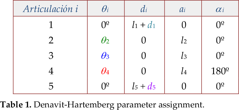
In order to obtain the kinematic model, we have considered the standard Denavit-Hartemberg method, whose parameters are listed in Table 1.
Denavit-Hartemberg parameter assignment.
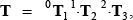
Then, applying the homogeneous transformations given by Eqs. (3) and (4), we obtain the direct kinematic model given by the matrix (5):


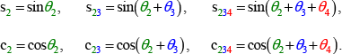
where:
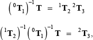
In order to obtain inverse kinematics in a redundant robot we must consider different methods, selecting the most adequate one in accordance with model considerations. If we use homogeneous transformation matrices it is necessary to clear the n “q variables”, in terms of vector components

where the tij elements are functions of the joints coordinates [q1, …, qn]
T
, and in this way it is possible to think that by means of some combinations of the 12 equations presented in (6) we can clear the n “q joints variables” in terms of the vector components
rearranging, we obtain:
since
When applying this method to the three rotational degrees of freedom that rules the robot's movement in the plane x-y, as shown in Fig. 5, multiple solutions will be obtained. In order to overcome this limitation, we establish the condition stated by Eq. (9):

Scheme of the three rotational DOF in the SCARA-type redundant robot manipulator.

Accordingly with these considerations - and after adequate simplifications - the inverse kinematic model is obtained, expressed by:
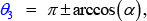


where z and d1 are known.
3.2 Dynamics
Having in mind the above presented manipulator, it is now necessary to obtain its dynamic model. For this purpose, we will employ the Lagrange-Euler formulation that is based on the principle of energy conservation [10]. Next, we need to obtain the manipulator's kinetic energy and potential energy. Therefore, to obtain the dynamic equation of the robotic manipulator, we must determine [11]:
manipulator's kinetic and potential energy,
the Lagrangian (Eq. (15)), and
to replace in Lagrange-Euler Equation (16),


where:
L: Lagrangian function (Lagrangian).
K: Kinetic energy.
U: Potential energy.
q: Vector of generalized (joint) coordinates.
q̇: Vector of generalized (joint) speeds.
τ: Vector of generalized forces (forces and torques).
In this way, the dynamic model of a manipulator with n joints can be expressed through Eq. (17) [9, 12, 13]:

where:
τ: Vector of generalized forces (n×1 dimension).
M: Inertia matrix (n×n dimension).
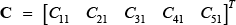
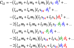
C: Vector of centrifugal and Coriolis forces (n×1 dimension).
q: Components of the joint position vector.
q̇: Components of the joint speed vector.
G: Vector of gravitational force (n×1 dimension).
q̈: Vector of joint acceleration (n×1dimension).
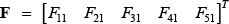
F: Vector of friction forces (n×1 dimension).
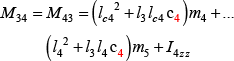
Therefore, from Eqs. (15), (16) and (17) the dynamic model of the redundant robotic manipulator can be expressed through Eqs. (18) to (35):
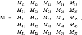


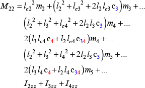
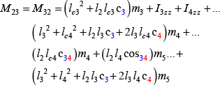


where:

m1: Mass of the first link.
m2: Mass of the second link
m3: Mass of the third link.
m4: Mass of the fourth link.
m5: Mass of the fifth link.
l1: Length of the first link.
l2: Length of the second link.
l3: Length of the third link.
l4: Length of the fourth link.
l5: Length of the fifth link.
lc2: Length from the origin of the 2nd link to its centroid.
lc3: Length from the origin of the 3rd link to its centroid.
lc4: Length from the origin of the 4th link to its centroid.
l2zz: Inertial momentum of the 2nd link with respect to the 1st z axis of its joint.
l3zz: Inertial momentum of the 3rd link with respect to the 1st z axis of its joint.
l4zz: Inertial momentum of the 4th link with respect to the 1st z axis of its joint.
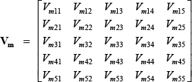
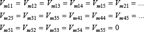
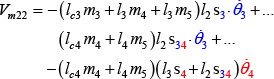
In the manipulator's dynamic model, as pointed in Eq. (17), the term corresponding to centrifugal and Coriolis forces is frequently expressed through a

According to this, the matrix


4. Actuator Dynamics
The actuators considered in this study are servo motors, which are composed by a direct current motor, a gear train for reducing spin speed and increasing torque in the drive shaft, a potentiometer connected to the output axis which is used to know a position, and a feedback control circuit which converts a PWM (Pulse-Width Modulation) input signal into voltage, compares it with the feedback position, and then amplifies it to drive an H-bridge so as to produce the spin at a specified speed [3].
In Figs. 6 and 7 we can see, respectively, a schematic diagram and a block diagram of a servomotor coupled to a robotic manipulator as a load [14].

Schematic diagram of a servomotor coupled to a robotic manipulator as a load.
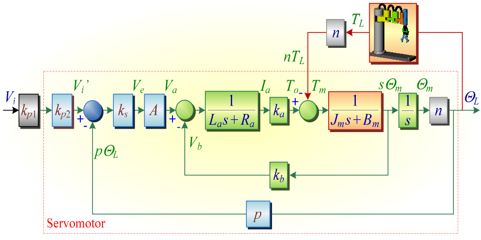
Block diagram of a servomotor coupled to a robotic manipulator as a load.
The dynamic model of the considered servo motors has been developed by authors in [14], and is given by expressions (47) and (48):


where:
n: Gear ratio (n1/n2).
ka: Motor torque constant.
Ra: Armature resistance.
A: Gain of the power amplifier (H bridge).
ks: Comparator sensibility.
kp: Total PWM (kp1 · kp2) conversion gain.
vi: Servomotor input voltage.
Jm: Motor inertial momentum.
kb: Inverse electromotive force constant.
Bm: Motor viscous friction.
p: Position potentiometer gain.
k: tanh function slope gain.
k is a constant used to increase or reduce the curve slope in the zero-crossing.
5. Considered Controllers
Next we present a summary of the controllers considered for model evaluation of the robot along with its actuators, with their respective performance.
6. Hyperbolic Sine-Cosine Controller
This controller, already presented in [15], is composed by a proportional part based on hyperbolic sine-cosine functions, a derivative part based on a hyperbolic sine, and gravity compensation, as pointed in Eqs. (49) and (50).


where:

Kp: Proportional gain matrix, diagonal and definite positive (n×n dimension).

Kv: Derivative gain matrix, diagonal and definite positive (n×n dimension).
qe: Joint position error vector (n×1 dimension).
qd: Joint desired position vector (n×1 dimension).
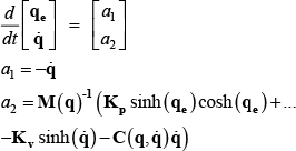
In [15] it is established that the robotic manipulator joint position error will asymptotically tend to zero as time approaches infinity:

this behavior is demonstrated by analyzing Eq. (54) and identifying that the system's only equilibrium point is the origin (0, 0).
6.1 Sliding Mode Controller
Sliding Mode Controllers (SMC) are a particular kind of Variable Structure Control (VSC) system with the ability to change structure by means of some law in order to satisfy the desired features [16]. SMC consists in defining a control law which - switching at a high frequency - drives the system's status into a surface called a “sliding surface”, keeping it in front of possible external perturbations [17]. One of the major advantages of the sliding mode control lies on its invariance against parameter uncertainties and external perturbations. Nevertheless, high switching frequencies usually cannot be implemented [18], and it also introduces to actuators the vibration phenomenon called “chattering”, which must be avoided in many physical systems, such as servo control systems, structure vibration control systems and robotic systems [19].
The control law corresponds to:
where:

K: Definite positive diagonal matrix (n×n dimension). and the sliding surface is given by:

where:
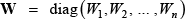
W: Definite positive diagonal matrix (n×n dimension).
6.2 Calculated Torque Controller
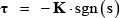
Another developed controller employs a control law by calculated torque, consisting in the application of a torque in order to compensate the centrifugal, Coriolis, gravitatory and friction effects, as stated in Eq. (59) [20]:

where:
M̂: Estimation of inertia matrix (n×n dimension).
Ĉ: Estimation of centrifugal and Coriolis forces vector (n×1 dimension).
Ĝ: Estimation of gravity force vector (n×1 dimension).
F̂: Estimation of friction forces vector (n×1 dimension).
Kv: Definite positive diagonal matrix (n×n dimension) defined in (52).
Kp: Definite positive diagonal matrix (n×n dimension) defined in (51).
qe: Joint position error vector (n×1 dimension) defined in (50).

q̇e: Joint speed error vector (n×1 dimension).
q̈d: Joint desired acceleration vector (n×1 dimension).
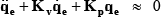
If the estimation errors are little, joints errors approach to a linear equation, as pointed in Eq. (61).
6. Simulation Environment
The three control laws above mentioned, along with the SCARA-type redundant manipulator dynamic model and the actuator dynamics, were run in a simulation structure, created by means of MatLab/Simulink programming tools, as shown in Fig. 8.

Block diagram of the simulator employed to test the manipulator model along with the mentioned control laws.
Parameter values considered for the manipulator are displayed in Table 2.
Parameters considered for the manipulador.

Table 3. shows the set of parameter values used for each actuator.
Parameters considered for servo motors.

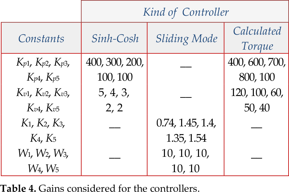
Table 4. shows the set of gain values employed for each kind of controller.
Gains considered for the controllers.
7. Results
After developing the manipulator model and the simulation environment - including the actuator dynamics - and establishing the control laws to be used, a test trajectory was determined in the space to subject the manipulator's model to path tracking, and we then studied the results in terms of the performance of each controller. This trajectory is shown in Fig. 9.

Test Cartesian desired trajectory.
Figs. 10, 11 and 12 show the curves corresponding to comparisons between the desired Cartesian trajectory and the real Cartesian trajectory, displaying the views in space, plane x-y and plane y-z, respectively. All of this is under the action of the hyperbolic sine-cosine controller, where:

Comparison in the space of the desired and real Cartesian trajectories using the hyperbolic sine-cosine controller.

Comparison in plane x-y of the desired and real Cartesian trajectories using the hyperbolic sine-cosine controller.
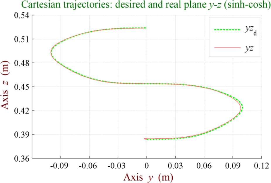
Comparison in plane y-z of the desired and real Cartesian trajectories using the hyperbolic sine-cosine controller.
xyzd: Desired Cartesian trajectory, in space.
xyz: Real Cartesian trajectory, in space.
xyd: Desired Cartesian trajectory, in plane x-y.
xy: Real Cartesian trajectory, in plane x-y.
yzd: Desired Cartesian trajectory, in plane y-z.
yz: Real Cartesian trajectory, in plane y-z.
In Fig. 13 are seen the curves corresponding to desired and real joint trajectories, when using the hyperbolic sine-cosine controller, where:

Comparison of the real and desired joint trajectories using the hyperbolic sine-cosine controller.
qdn: Desired joint trajectory, where n represents joints 1 to 5.
qn: Real joint trajectory, where n represents joints 1 to 5.
Forces and torques supplied to the robot by actuators, under the action of hyperbolic sine-cosine controller, are shown in Fig. 14, where:
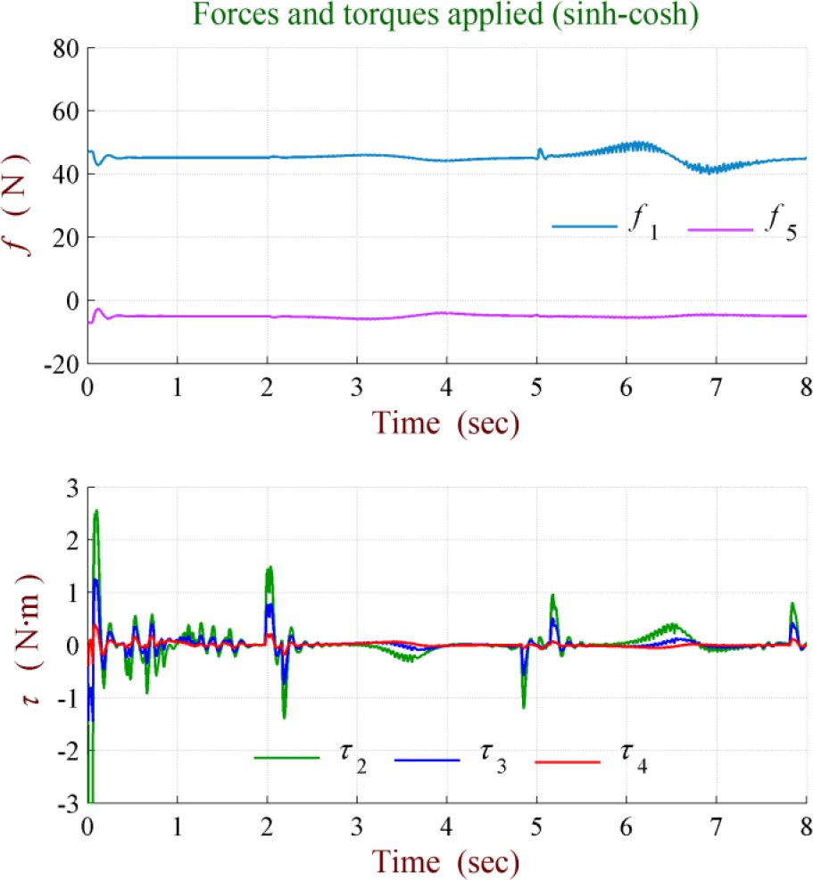
Forces and torques applied to the robot when using the hyperbolic sine-cosine controller.
f1: Force applied in joint 1.
τ2: Torque applied in joint 2.
τ3: Torque applied in joint 3.
τ4: Torque applied in joint 4.
f5: Force applied in joint 5.
Figs. 15 and 16 display the errors obtained from desired and real Cartesian trajectories, and desired and real joint trajectories, respectively, when using the hyperbolic sine-cosine controller, where:
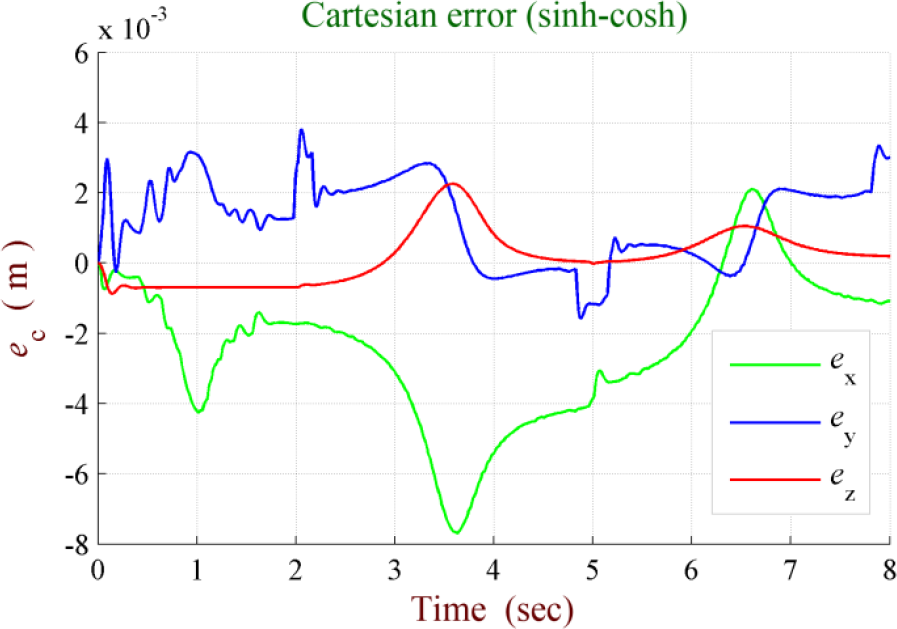
Cartesian trajectory error, when using the hyperbolic sine-cosine controller.

Joint trajectory error, when using the hyperbolic sine-cosine controller.
ex: Error in Cartesian trajectory, x axis.
ey: Error in Cartesian trajectory, y axis.
ez: Error in Cartesian trajectory, z axis.
en: Error in joint trajectory, where n represents joints 1 to 5.
Comparisons between the desired and real Cartesian trajectories, under the sliding mode controller, are shown in Figs. 17, 18 and 19, displaying the charts corresponding to the space, the plane x-y and the plane y-z, respectively.

Comparison in the space of the desired and real Cartesian trajectories using the sliding mode controller.

Comparison in plane x-y of the desired and real Cartesian trajectories using the sliding mode controller.

Comparison in the plane y-z of Cartesian desired and real trajectories using the sliding mode controller.
In Fig. 20 we display the charts related to joint desired and real trajectories when using the sliding mode controller.

Comparison of the joint desired and real trajectories when using the sliding mode controller.
Fig. 21 shows the response of the actuators, indicating forces and torques developed during trajectory tracking, when using the sliding mode controller.
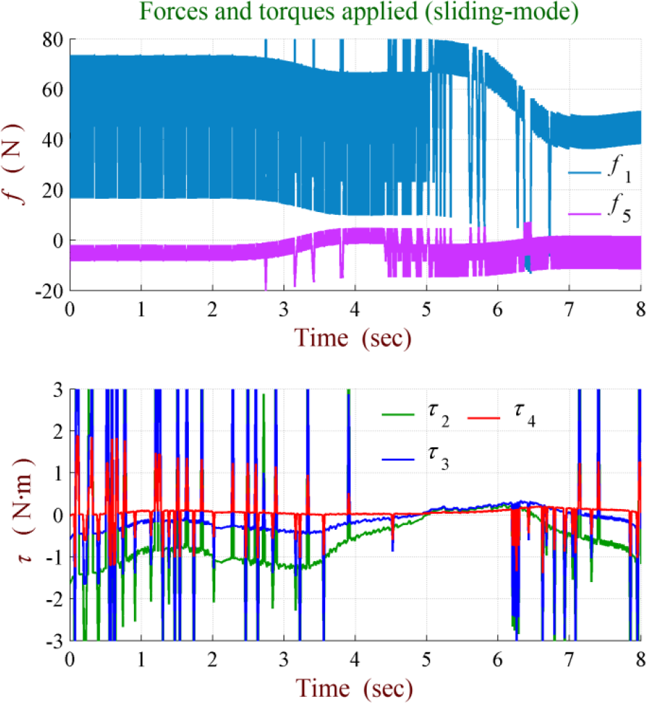
Forces and torques applied to the robot when using the sliding mode controller.
Errors produced by the difference between the desired and real Cartesian trajectories and the joint desired and real trajectories when applying the sliding mode controller, are shown in Figs. 22 and 23, respectively.
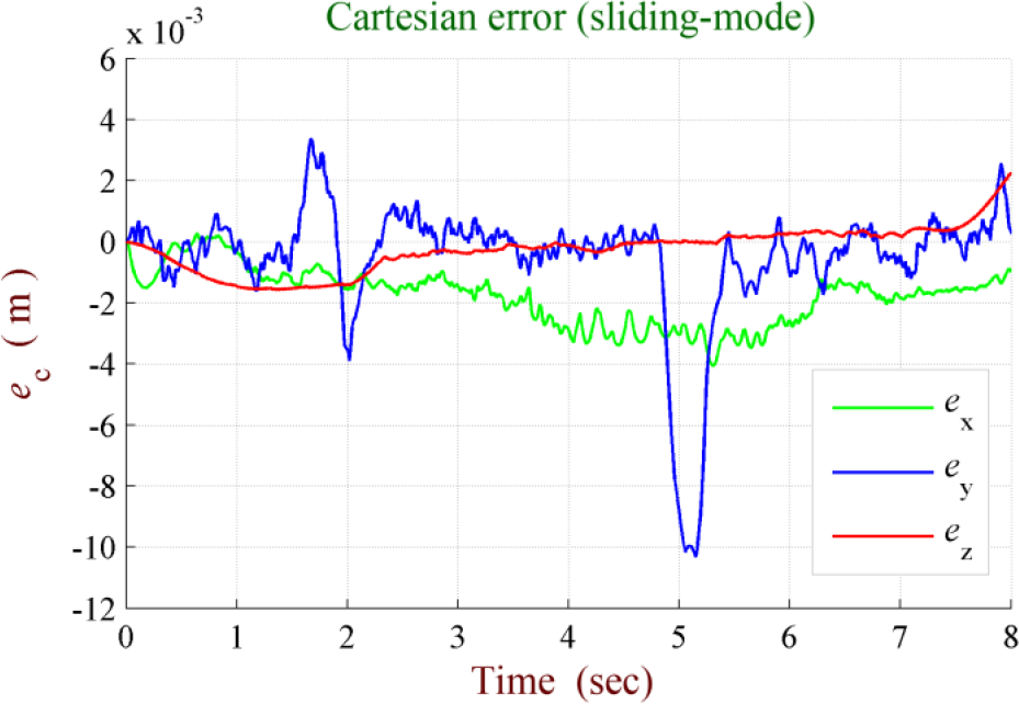
Error in Cartesian trajectory when using the sliding mode controller.
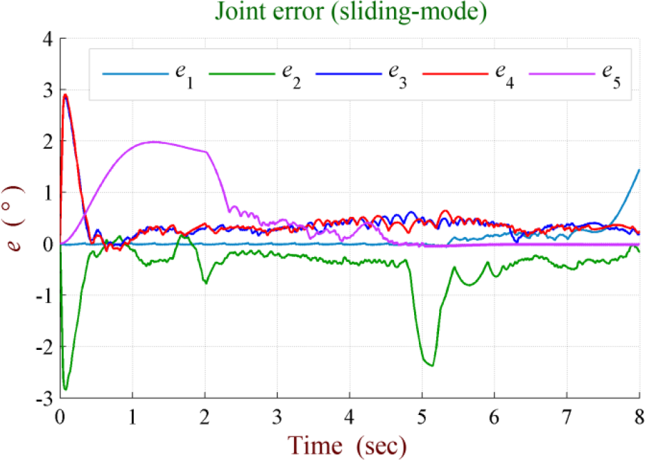
Error in joint trajectory when using the sliding mode controller.
The tracking response of robot model in the joint space, when using the calculated torque controller, is shown in Figs. 24, 25 and 26, displaying the desired and real curves in the space, the plane x-y and the plane y-z, respectively.

Comparison in the space of the desired and real Cartesian trajectories when using the calculated torque controller.
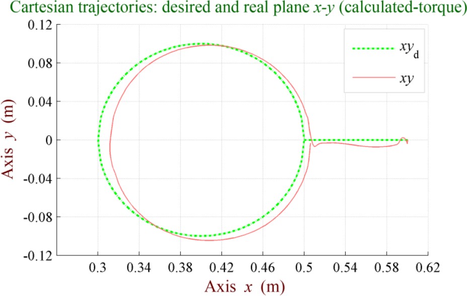
Comparison in plane x-y of the desired and real Cartesian trajectories when using the calculated torque controller.
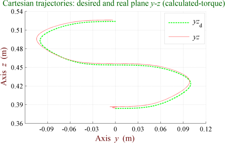
Comparison in plane y-z of the desired and real Cartesian trajectories when using the calculated torque controller.
Comparisons between joint desired and real trajectories under the calculated torque controller are shown in Fig. 27.
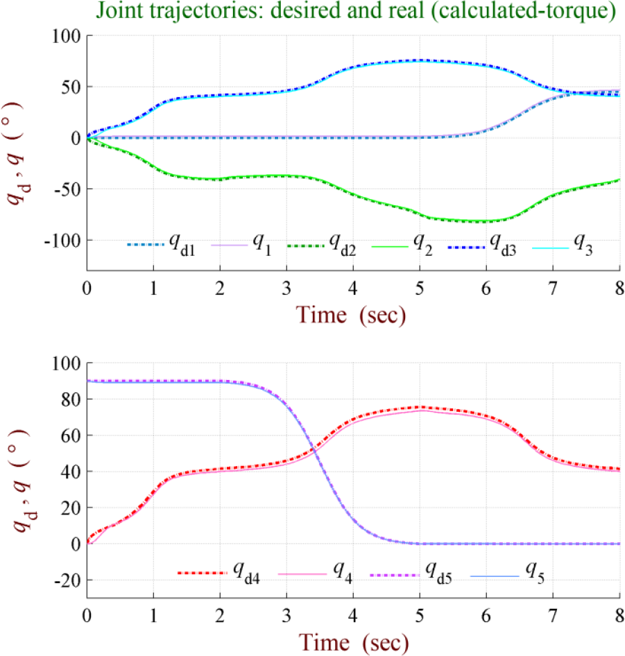
Comparison of the joint desired and real trajectories when using the calculated torque controller.
In Fig. 28 are seen the curves corresponding to the forces and torques applied by servo motors under the application of the calculated torque controller.
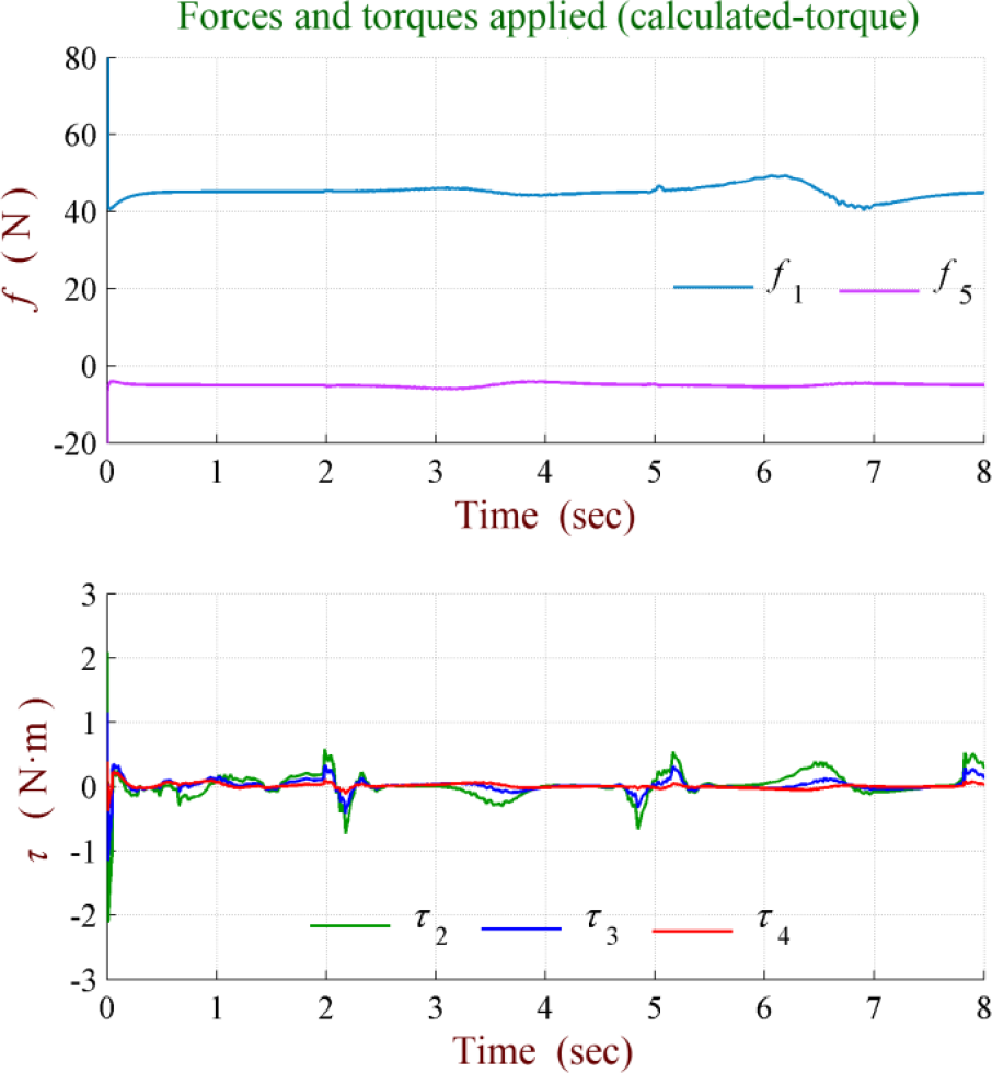
Forces and torques applied to the robot when using the calculated torque controller.
In Figs. 29 and 30, we can see the error curves obtained from Cartesian and joint desired and real trajectories when using the calculated torque controller.

Error in Cartesian trajectory when using the calculated torque controller.
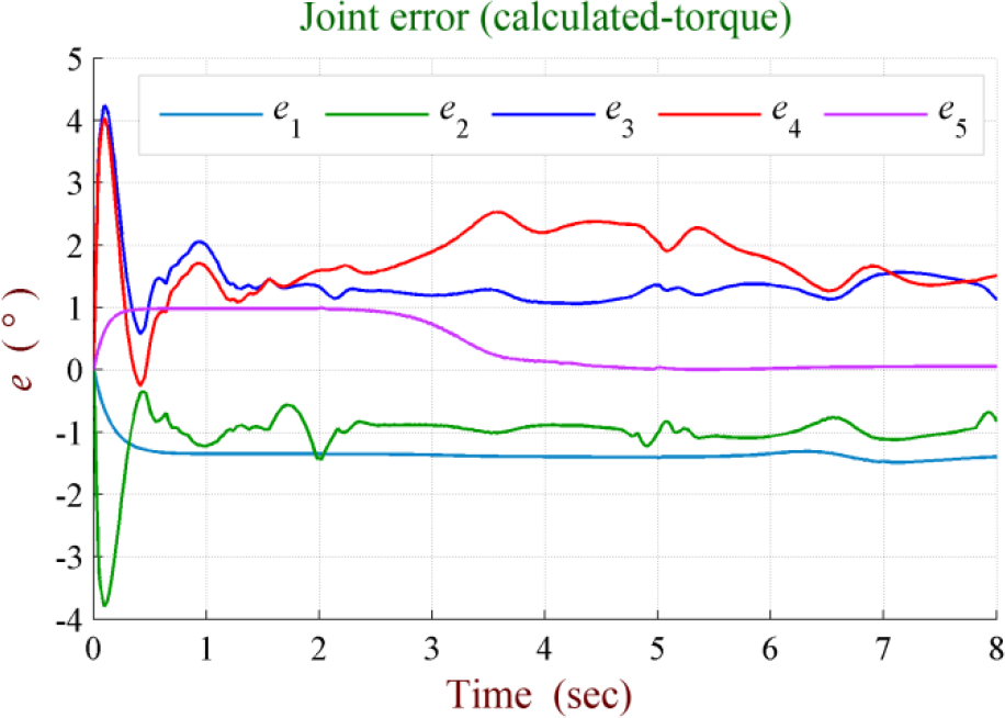
Error in joint trajectory when using the calculated torque controller.
Finally, figs. 31 and 32 show joint and Cartesian rms errors, respectively, in accordance with Eq. (62).

Performance index corresponding to joint trajectory.

Performance index corresponding to the Cartesian trajectory.

Where ei represents both the joint and Cartesian trajectory errors and n is the number of data.
8. Conclusions
In this paper, we developed the kinematic and dynamic model of a redundant SCARA-type manipulator robot with five degrees of freedom using the Denavit-Hartemberg and Lagrange-Euler methods, respectively. Three controllers were developed: hyperbolic sine-cosine, sliding mode and calculated torque. A simulator was also created, using the MatLab/Simulink software. Several tests on this model were presented, including actuator dynamics under each controller through a path tracking test consisting of a spiral in the Cartesian space. The results obtained through the simulation environment were displayed by means of comparative curves and an rms index for joint and Cartesian errors.
From the results obtained, we can see that the redundant manipulator model presented a path tracking response whose maximum errors were less severe when using the hyperbolic sine-cosine controller than in the other two cases, leading to more homogeneous manipulator movements. We also appreciate that the greatest joint and Cartesian errors produced when testing the robot model, both for maximum and rms values, occurred when using the calculated torque controller. Consequently, the best results for the robotic manipulator's model performance were obtained when applying the hyperbolic sine-cosine controller, as shown in Figs. 31 and 32. It is important to notice that both the hyperbolic sine-cosine and the sliding mode controllers present a lesser simulation complexity, since they do not require the second derivative of joint position. Such a condition can be decisive in the case of not having high-performance processors. The practical implementation of the sliding mode controller, however, has a considerable disadvantage: the controller's high switching frequency, leading to a remarkable deterioration of the actuators.
9. Further Research
From the behavior obtained through the simulation tests for the redundant robot model with its actuators and the different control laws that were analyzed, we can begin a new stage in the study and analysis of redundant robotic manipulators, consisting in the practical implementation of real industrial-type robots, its actuators and controllers, by means of the development of the proper hardware, as is schematized in Figs. 33 and 34.
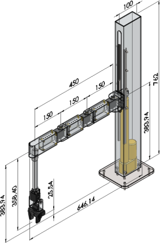
Scheme of a SCARA-type redundat robot (view A).

Scheme of a SCARA-type redundant robot (view B).
Footnotes
10. Acknowledgements
This work had the support of the Department of Scientific and Technologic Research of the Universidad de Santiago de Chile, through Project 060713UO.