Sage Journals: Discover world-class research

Abstract

This paper presents a decoupled nonsingular terminal sliding mode controller (DNTSMC) for a novel 3-DOF parallel manipulator with actuation redundancy. According to kinematic analysis, the inverse dynamic model for a novel 3-DOF redundantly actuated parallel manipulator is formulated in the task space using Lagrangian formalism and decoupled into three entirely independent subsystems under generalized coordinates to significantly reduce system complexity. Based on the dynamic model, a decoupled sliding mode control strategy is proposed for the parallel manipulator; the idea behind this strategy is to design a nonsingular terminal sliding mode controller for each subsystem, which can drive states of three subsystems to the original equilibrium points simultaneously by two intermediate variables. Additionally, a RBF neural network is used to compensate the cross-coupling force and gravity to enhance the control precision. Simulation and experimental results show that the proposed DNTSMC can achieve better control performances compared with the conventional sliding mode controller (SMC) and the DNTSMC without compensator.

Keywords

parallel manipulator redundant actuation dynamics modelling coupling analysis nonsingular terminal sliding mode control decoupled control

1. Introduction

A parallel manipulator is essentially a closed-loop kinematic chain mechanism in which the end-effector is linked to the base by several independent kinematic chains [1]. Due to the distinct advantages such as low inertia, high stiffness, high accuracy and identical behaviours in each axis [2], it has attracted significant attention amongst researchers in the past decade, and has been utilized for efficient machines in industrial applications where high structural stiffness, high velocity and good dynamic performance are predominant requirements, such as in assembly, packaging and machining operations [3].

As is well known, the parallel manipulator is a complicated multivariable nonlinear strong-coupling system. The mechanical structure of the parallel manipulator contains a number of interconnected branch chains, and the performances of the end-effector are contributed to by its independent actuators. Because there are nonlinear couplings among each driving chain, serious degradation of performance often happens, especially when the parallel manipulator moves with large amplitudes and high velocity. So, the designed controller in each chain should consider the coupling impact from other chains with interconnections [4]. Eliminating or reducing the coupling of parallel manipulators can improve system control accuracy and trajectory tracking performance in all DOFs [5]. Reviewing the literature, it is of note that many scholars devote themselves to the kinematic design of the decoupled parallel manipulator; however, few of them explicitly consider the decoupled control methods of the system [6, 7]. In [5], the feedback linearization theory is applied to reduce coupling effects stemming from the system dynamics of the parallel robot by incorporating force-velocity control with cross-coupling pre-compensations. In [8], a proportional plus derivative controller with dynamic gravity compensation (PDGC) is developed to improve control performances including steady and dynamic precision via compensating for steady state errors and reducing dynamic errors for a 6-DOF hydraulic driven parallel manipulator. In [9], according to the characteristics of a dynamics model for the 3-RRRT parallel robot, an improved computed torque decoupled control method was presented through calculating moments to improve the control precision. In terms of the control algorithm, the traditional PD controller including the augmented PD (APD) controller and the computed torque (CT) controller mentioned above are the preferred control schemes for the parallel manipulator in practice; however, they cannot always ensure better control performances by virtue of the strong coupling and high nonlinearity of such a system with parameter uncertainties and unmodelled dynamics [10]. Hence, there is a need to propose control strategies with robustness, adaptive capability, fast convergence and a simple structure. In the last few decades, research efforts have been devoted to the design or improvement of the controller for uncertain systems. Among these control strategies, the sliding mode control (SMC) is a well established technique for the control of uncertain systems acted upon by unmeasurable disturbance, which does not depend on the accurate mathematical model of the controlled object and has various attractive features such as guaranteed stability, robustness against parameter variations, fast dynamic response and simplicity in implementation [11]. Therefore, it has been widely applied to parallel manipulators. Furthermore, with features of intelligent control theory, many researchers have been attempting to use intelligent control approaches to represent complex plants and construct advanced controllers to further enhance control performance [12]. Wu [13] et al. designed adaptive sliding control for parallel manipulators. Achili [14], combining a neural network and sliding mode technique for parallel robots control, adopted the robust controller with respect to external disturbances in order to improve trajectory tracking. Gao et al. proposed chattering-free sliding mode control [15], and synchronous smooth sliding mode control [16] to improve the control performances of a 2-DOF and 6-DOF parallel robot with strong coupling and high non-linearity.

In most SMC schemes, the most commonly used sliding surface is the linear sliding surface, which is based on a linear combination of system states by using an appropriate time-invariant coefficient. Although the convergence rate can be made faster by adjusting the coefficient, the system states in the sliding mode cannot converge to equilibrium point in finite time [17]. In order to achieve finite time convergence of the system states, a terminal sliding mode control (TSMC) approach was proposed by Zak and Man et al., and has been used in various control problems [18, 19]. In [20], a robust multi-input/multi-output (MIMO) terminal sliding mode control technique is firstly developed for n-link rigid robotic manipulators and the relationship between the terminal switching plane variable vector and system error dynamics is established. In [21], an adaptive terminal sliding mode control (ATSMC) strategy is presented for DC–DC buck converters. The idea behind this strategy is to use the terminal sliding mode control (TSMC) approach to assure finite time convergence of the output voltage error to the equilibrium point and integrate an adaptive law to the TSMC strategy so as to achieve a dynamic sliding line during load variations. The developed TSMC assures a finite convergence time for MPP tracking. However, for the parallel manipulator system, the TSMC will suffer from the singularity problem, which can generate an unbounded control signal and should be avoided. Feng et al. [22] proposed a global nonsingular terminal sliding mode controller for rigid manipulators. In [19], a nonsingular decoupled terminal sliding mode control (NDTSMC) is proposed for a class of fourth-order systems. In [23], a continuous nonsingular terminal sliding mode control approach is proposed for mismatched disturbance attenuation and a novel nonlinear dynamic sliding mode surface is designed based on a finite time disturbance observer.

This paper presents a decoupled nonsingular terminal sliding mode controller (DNTSMC) for a novel 3-DOF parallel manipulator with actuation redundancy. The idea behind this strategy is to decouple the whole system into three subsystems under generalized coordinates and to design a nonsingular terminal sliding mode controller for each subsystem, which can drive the states of three subsystems to the original equilibrium points simultaneously by two intermediate variables. Additionally, a RBF neural network is used to compensate the cross-coupling force and gravity to enhance control precision. Simulation and experimental results show that the proposed method can achieve good control performance.

2. Model of parallel manipulator

2.1 Structure description

The prototype of the hybrid machine tool is shown in Figure 1., which is composed of a 3-DOF parallel manipulator with actuation redundancy and a serial worktable [24]. In this paper, the 3-DOF parallel manipulator is the main research object and its dynamics and control method are the research focus.

Figure 1.

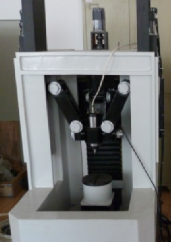
Prototype of hybrid machine tool

The parallel manipulator consists of one moving platform, three identical chains and four sliders. Each of the chains consists of a length-fixed link, which is connected to the active slider through a passive revolute joint and is connected to the moving platform through a universal joint. The whole construction of the parallel manipulator enables the movement of the moving platform in two directions (Y and Z axes) and rotation about the axis norm to the O–YX plane; then, the parallel manipulator has three spatial freedoms. Furthermore, the moving platform can tilt continuously from −25° to 90°. For this reason, by adding the serial worktable the mechanism is capable of four-face machining [25, 26].

2.2 Inverse kinematics analysis

The kinematic model of the 3-DOF parallel manipulator with actuation redundancy has been developed by Tsinghua University, as shown in Figure 2, where, the points B_i are the centres of the universal joints that connect the legs to the base, and the points P_i are the centres of the universal joints that connect the legs to the platform with i=1,2,3. 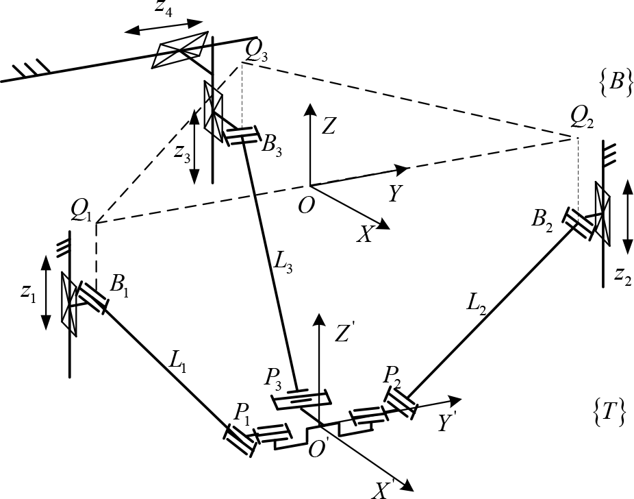For the following analytical developments, it is convenient to define a fixed frame { B } and a moving frame { T }, which are attached to the centre of the side B₁B₂ and P₁P₂ respectively. Then the configuration of the platform can be described by the coordinates (0, y, z) with respect to the moving frame, and the rotational angle β from the Z′-axis to the Z-axis. Thus, the following generalized coordinates q=[y, z, β]^T can be chosen to describe the pose of the 3-DOF parallel manipulator [26].

Figure 2.

Kinematic model of the parallel manipulator

By analysis, the coordinate position of point B_i(i=1,2,3) in frame { B } can be denoted as

B_{1} = (\begin{matrix} 0 \\ - R_{1} \\ z_{1} \end{matrix}), B_{2} = (\begin{matrix} 0 \\ R_{2} \\ z_{2} \end{matrix}), B_{3} = (\begin{matrix} - R_{3} \\ y \\ z_{3} \end{matrix})

(1)

where R_i(i =1,2,3) is the distance from point Q_i to point O.

The coordinate position of point P_i in frame { T } can be expressed as

{P^{'}}_{1} = (\begin{matrix} 0 \\ - r_{1} \\ 0 \end{matrix}), {P^{'}}_{2} = (\begin{matrix} 0 \\ r_{2} \\ 0 \end{matrix}), {P^{'}}_{3} = (\begin{matrix} - r_{3} \\ 0 \\ 0 \end{matrix})

(2)

where r_i(i=1,2,3) is the distance from point P_i to point O′.

Then, the coordinate position of point Pi in frame { B } can be obtained as

P_{i} = T_{M}^{B} P_{i}^{'} + O_{M}^{B}

(3)

where O^B_M is coordinate position of the origin O′ in frame { B } and T^B_M^B is the coordinate transformation matrix between frames { T } and { B }.

So, the coordinate position of point P_i in frame { B } can be obtained, as follows

P_{1} = (\begin{matrix} 0 \\ y - r_{1} \\ z \end{matrix}), P_{2} = (\begin{matrix} 0 \\ y + r_{2} \\ 0 \end{matrix}), P_{3} = (\begin{matrix} - r_{3} \cos β \\ y \\ z + r_{3} \cos β \end{matrix})

(4)

According to the mechanical character of L_i²=‖OB_i-OP_i‖², the constraint equations for the three kinematic chains are described as

{\begin{array}{l} {(y - r + R)}^{2} + {(z - z_{1})}^{2} = L_{1}^{2} \\ {(y + r - R)}^{2} + {(z - z_{2})}^{2} = L_{2}^{2} \\ {(- R_{3} + r_{3} \cos β)}^{2} + {(z_{3} - r_{3} \sin β - z)}^{2} = L_{3}^{2} \end{array}

(5)

Then, the inverse kinematic solution can be obtained, as follows

{\begin{array}{l} z_{1} = \pm \sqrt{L_{1}^{2} - {(y - r + R)}^{2}} + z \\ z_{2} = \pm \sqrt{L_{2}^{2} - {(y + r - R)}^{2}} + z \\ z_{3} = \pm \sqrt{L_{3}^{2} - {(R_{3} - r_{3} \cos β)}^{2}} + r_{3} \sin β + z \end{array}

(6)

From (6), it is noted that there are eight inverse kinematics solutions for a given pose. To obtain the inverse configuration as shown in Fig. 1, each of the signs ‘±’ in (6) should be chosen as ‘+’.

The redundant actuated slider can only drive the third chain to move in the Y direction, and there is no relative motion between the redundant actuated slider and the moving platform in the Y direction. So, the displacement of the redundant actuated slider can be obtained by z₄=y. However, when the driving motor rotates forward, the redundant actuated slider moves along the negative direction of Y-axis, which yields

z_{4} = - y

(7)

The (7) and (8) are the inverse kinematics for the 3-DOF parallel manipulator with actuation redundancy [25,26].

3. Dynamic modelling

Dynamics plays an important role in the application of parallel manipulators. In order to investigate the dynamic characteristics of parallel manipulators, it is necessary to derive the dynamic model prior to the implementation of a control scheme [27]. In order to obtain a more compact form of the dynamic model for the implementation of real-time control, neglecting the friction forces and considering the gravitational effects system, the Lagrange formalism is employed to derive the dynamic model. Here, all the kinematic parameters are described relative to the fixed Cartesian frame { B }. Moreover, we suppose that the centre of mass is in the centres of geometry; each component is simplified as a homogeneous rectangular body, and then the inertia of each component can be computed.

3.1 Kinetic energy

The kinetic energy of a moving platform can be divided into two terms, translational energy and rotational kinetic energy, expressed as

T_{p} = \frac{1}{2} m_{p} ({\dot{y}}^{2} + {\dot{z}}^{2}) + \frac{1}{2} ω_{h} ​^{T} I_{p} ω_{h} ​^{T}

(8)

where m_p,ω_h and I _p are the mass, the angular velocity and the moment of inertia of the moving platform.

The three legs perform both translational and rotational motions, but in practice the angular velocity of each leg is too small to be ignored. The total kinetic energy of three legs can be described as

T_{l} = \sum_{i = 1}^{3} \frac{1}{2} m_{l i} v_{G i}^{T} v_{G i}

(9)

where, m_liand v_Gi (i=1,2,3) are the mass and linear velocity of linkage.

In the frame { B }, assume that the leg B_iP_i (i=1,2,3) is a homogeneous body and the coordinate position for the centre of mass is denoted as G_i, then

G_{i} = \vec{O P_{i}} + \frac{1}{2} L_{i} \vec{u_{i}}

(10)

where $\vec{u_{i}} = \frac{\vec{P_{i} B_{i}}}{L_{i}}$ is the unit vector for the ith leg. Substituting (1) and (5) into (10) yields

\begin{array}{l} G_{1} = {[0, \frac{1}{2} (y - r + R), z + \frac{1}{2} \sqrt{L_{2} ​^{2} - {(y - r + R)}^{2}}]}^{T} \\ G_{2} = {[0, \frac{1}{2} (y + r - R), z + \frac{1}{2} \sqrt{L_{2} ​^{2} - {(y + r - R)}^{2}}]}^{T} \\ G_{3} = {[- \frac{1}{2} R_{3} - \frac{1}{2} r_{3} \cos β, y, z + r_{3} \sin β + \frac{1}{2} \sqrt{L_{3} ​^{2} - {(R_{3} - r_{3} \cos β)}^{2}}]}^{T} \end{array}

(11)

Take a derivative of (11) with respect to t and the linear velocities v_Gi can be obtained.

Moreover, the driving sliders perform only translational motion, so the kinetic energy for four sliders can be described as

T_{b} = \sum_{i = 1}^{4} \frac{1}{2} m_{b i} v_{b i}^{T} v_{b i}

(12)

where m_bi, v_bi (i=1,2…4) are the mass and the linear velocity for the ith slider, respectively.

Then the total kinetic energy for the whole parallel manipulator can be described as

T = T_{p} + T_{l} + T_{b}

(13)

3.2 Potential energy

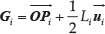
Choose the XOY plane of frame { B } as the zero potential energy plane, and the potential energy for the moving platform, the kinematic legs and the driving sliders can be described as follows

\begin{array}{l} U_{p} = m_{p} g z \\ U_{l} = \sum_{i = 1}^{3} m_{l i} g z_{G_{i}} \begin{matrix} (i = 1, 2 \dots 3) \end{matrix} \\ U_{b} = \sum_{i = 1}^{3} m_{b i} g z_{i} \begin{matrix} (i = 1, 2 \dots 3) \end{matrix} \end{array}

(14)

where z_Gi is the coordinates in the Z-axis for the centres of mass for the ith leg.

The gravity of the redundant drive slider is counteracted by the support force of the manipulator frame. Then, the total potential energy of the whole parallel manipulator can be described as [26]

U = U_{p} + U_{l} + U_{b}

(15)

3.3 Dynamic formulation

According to the analysis mentioned above, in Cartesian coordinates the dynamics of the parallel manipulator is governed by

M (q) \overset{..}{q} + C (q, \dot{q}) \dot{q} + G (q) = τ = J^{T} F

(16)

where M(q) is the inertia matrix; C(q, q̇) is the Coriolis and centrifugal force terms; G(q) is the gravity force terms; $τ = {[τ_{1}, τ_{2}, τ_{3}]}^{T}$ is the equivalent generalized force vector in the Y, Z and β direction; F=[f₁, f₂, f₃, f₄]^T is the driving force vector that acts on the four sliders; J is the Jacobian matrix. The detailed expressions for M (q), C(q, q̇), G(q) and J are given explicitly in [28].

Since the parallel manipulator has one redundant actuator and J^T is non-square, the driving force F in (16) has infinite solutions. To obtain a unique solution, an optimization technique has to be applied. In this paper, the optimizing objective is to minimize the 2-norm of τ [29], so

F = {(J^{T})}^{+} τ

(17)

where (J^T)+=J(J ^TJ)¹ is the Moore-Penrose inverse of J^T, satisfying J (J^T)⁺=I and (J)⁺ J^T=I.

In practice, for the 3-DOF parallel manipulator system, the external disturbances such as friction torque between the joints, the servo system friction, the environmental noise and the unmodelled dynamics are inevitable, which will make a strong impact on the performance of the parallel manipulator, so the dynamic formulation shown in (16) can be rewritten as

M (q) \overset{..}{q} + C (q, \dot{q}) \dot{q} + G (q) = τ - τ_{d}

(18)

Where $τ_{d} = {[τ_{d 1}, τ_{d 2}, τ_{d 3}]}^{T}$ is the vector of lumped uncertainty including the unmodelled dynamics and external disturbance [26].

4. Controller design

4.1 Control strategy

It is noted from Eq. (18) that the parallel manipulator with actuation redundancy is a complex system with time-varying, highly nonlinear, and strong coupling characteristics. The time-consuming computing for the parallel manipulator system is the bottleneck of real-time control based on dynamics. In this section, the entirely decoupled sliding mode controller (NDTSMC) is proposed with cross-coupling forces and dynamical gravity terms compensation. The principle of this approach consists of decoupling the whole system into three subsystems under generalized coordinates and controlling them independently. Then, the nonsingular sliding mode controllers are designed to drive the system states to the original equilibrium points simultaneously by two intermediate variables in finite time. The block diagram of the control system is shown in Figure. 3.

Figure 3.

Diagram of synchronization adaptive sliding mode control scheme

Where q_d=[y_d, z_d, β_d]T is the desired pose vector of the end-effector for the parallel manipulator, q=[y, z, β]^T is the actual pose vector, z₁ and z₂ are the intermediate variables and d̂(t) is the estimation of disturbance. It is of note that the RBF network used as the compensator has nine inputs and the last three inputs are accelerations; then, the acceleration feedback will result in an algebraic loop, but here a delay block is introduced to prevent the algebraic loop.

4.2 Design of nonsingular terminal sliding mode control

Through analysis, Eq. (18) can be rewritten as follows

{\begin{cases} τ_{1} = M_{11} \overset{..}{y} + C_{11} \dot{y} + τ_{d 1} + τ_{c c y} + G_{1} \\ τ_{2} = M_{22} \overset{..}{z} + C_{22} \dot{z} + τ_{d 2} + τ_{c c z} + G_{2} \\ τ_{3} = M_{33} \overset{..}{β} + C_{33} \dot{β} + τ_{d 3} + τ_{c c β} + G_{3} \end{cases}

(19)

Where $τ_{c c} = {[τ_{c c y}, τ_{c c z}, τ_{c c β}]}^{T}$ is the cross-coupling force vector, here, $τ_{c y}, τ_{c z}, τ_{c β}$ are the coupling forces for Y, Z and β directions, respectively, which are expressed as follows

{\begin{cases} τ_{c c y} = M_{12} \overset{..}{z} + C_{12} \dot{z} + M_{13} \overset{..}{β} + C_{13} \dot{β} \\ τ_{c c z} = M_{21} \overset{..}{y} + C_{21} \dot{y} + M_{23} \overset{..}{β} + C_{23} \dot{β} \\ τ_{c c β} = M_{32} \overset{..}{z} + C_{32} \dot{z} + M_{31} \overset{..}{y} + C_{31} \dot{y} \end{cases}

(20)

With the cross-coupling force τ_cc and the gravity force G(q) not being considered, the dynamic model in (18) can be expressed as

M' \overset{..}{q} + C' \dot{q} = τ - τ_{d}

(21)

Where M′=diag[M₁₁, M₂₂ a _, M₃₃] _; C′=diag[C ₁₁, C _22, C₃₃].

Then, the mathematical model used to describe the parallel manipulator movement in Y, Z and β te directions can be written in the following form

{\begin{cases} \overset{..}{y} = - \frac{C_{11}}{M_{11}} \dot{y} + \frac{1}{M_{11}} τ_{1} - \frac{1}{M_{11}} τ_{d 1} \\ \overset{..}{z} = - \frac{C_{22}}{M_{22}} \dot{z} + \frac{1}{M_{22}} τ_{2} - \frac{1}{M_{22}} τ_{d 2} \\ \overset{..}{β} = - \frac{C_{33}}{M_{33}} \dot{β} + \frac{1}{M_{33}} τ_{3} - \frac{1}{M_{33}} τ_{d 3} \end{cases}

(22)

Let $x_{1} = y, x_{2} = \dot{y}, x_{3} = z, x_{4} = \dot{z}, x_{5} = \dot{β}, x_{6} = \overset{..}{β}$ and take system uncertainty and external disturbance into account; the parallel manipulator system shown in (22) can be rewritten in abbreviated form as

{\begin{cases} {\dot{x}}_{1} = x_{2} \\ {\dot{x}}_{2} = f_{1} (x_{1}, x_{2}) x_{2} + b_{1} (x_{1}, x_{2}) τ_{1} + d_{1} (t) (a) \\ {\dot{x}}_{3} = x_{4} \\ {\dot{x}}_{4} = f_{2} (x_{3}, x_{4}) x_{4} + b_{2} (x_{3}, x_{4}) τ_{2} + d_{2} (t) (b) \\ {\dot{x}}_{5} = x_{6} \\ {\dot{x}}_{6} = f_{3} (x_{5}, x_{6}) x_{6} + b_{3} (x_{5}, x_{6}) τ_{3} + d_{3} (t) (c) \end{cases}

(23)

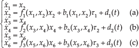
Where X=[x₁, x₂, x₃, x₄, x₅, x₆]^T is the state vector; f_i and b_i (i=1,2…3) are the nonlinear functions representing system dynamics with $f_{i} = - \frac{C_{i i}}{M_{i i}}, b_{i} = - \frac{1}{M_{i i}}; τ = {[τ_{1}, τ_{2}, τ_{3}]}^{T}$ is the control input vector meaning the _ii driving force in generalized c^oordinates; d = [d₁^, d₂, d₃]^T represents the external disturbance with $d_{i} = - \frac{1}{M_{i i}} τ_{d i}$ and the disturb ance is assumed to be bounced as ‖d‖ ≤D(t).

It is noted that the nonlinear six order system expressed in Eq. (23) includes three entirely independent second-order subsystems in canonical form with states [x₁, x₂]^T, [x₃, x₄]^T and [x₅, x₆]^T, which can describe the motion characteristics in Y, Z and β directions respectively. The basic ideal of the decoupled sliding mode control is to design control law for each subsystem to accomplish the desired performance. However, as the movement of the end-effector is closely related to each independent driving slider, we must consider the synchronization between subsystems when the controller is designed.

The subsystems in (23a), (23b) and (23c) are chosen as primary subsystem A, secondary subsystem B and a third subsystem C. The objective is to design a control strategy that would move the state of each subsystem toward its sliding mode surface, and simultaneously converge to the points [x₁, x₂]^T=[0, 0]^T, [x₃, x₄]^T=[0, 0]^T and [x₅, x₆]^T=[0, 0]^T respectively [30].

Define tracking errors e₁ = y_d−y, e₂=z_d−z, e₃=e β m_d−e β n and three nonlinear sliding surface functions, given by

{\begin{cases} s_{1} = {\dot{e}}_{1} + λ_{1} (e_{1} - z_{1})^{γ_{1}} (a) \\ s_{2} = {\dot{e}}_{2} + λ_{2} (e_{2} - z_{2})^{γ_{2}} (b) \\ s_{3} = {\dot{e}}_{3} + λ_{3} e_{3} ​^{γ_{3}} (c) \end{cases}

(24)

where λ_i(i = 1,2,3) is the positive constant, $γ_{i} = \frac{q_{i}}{p_{i}}$ with 0 γ_i < 1, p_i and q_i are positive odd integers and satisfy p_i >q_i. z₁, z₂ are the intermediate variables defined as

\begin{array}{l} z_{1} = s a t (\frac{s_{2}}{Φ_{Z_{2}}}) z_{U_{1}} \begin{matrix} 0 < z_{U_{1}} < 1 \end{matrix} \\ z_{2} = s a t (\frac{s_{3}}{Φ_{Z_{3}}}) z_{U_{2}} \begin{matrix} 0 < z_{U_{2}} < 1 \end{matrix} \end{array}

(25)

where Φ_Z₂ is the boundary layer of s₂ used to smooth z₁, and Φ_Z₃ is the boundary layer of s₃ used to smooth z_2.

It is clear from Eq. (25) that z₁ is a function of s₂ transforming s₂ to the proper range of e₁, and z₂ is a function of s₃ transforming s₃ to the proper range of e_2. This means that the sliding-mode condition s₂=0 for the subsystem B is incorporated into s₁ through the intermediate signal z₁ and s₃=0 for subsystem C is incorporated into s₂ through z₂. Hence, the control input that controls subsystems simultaneously can be obtained easily [31, 32]. Moreover, z₁ and z₂ are decaying oscillatory signal because z_U₁ and z_U₂ are factors less than 1.

Take the derivative of equations in Eq. (24) and equate them to zero, as follows

\begin{array}{l} {\overset{..}{e}}_{1} + λ_{1} γ_{1} (e_{1} - z_{1})^{γ_{1} - 1} ({\dot{e}}_{1} - {\dot{z}}_{1}) = 0 \\ {\overset{..}{e}}_{2} + λ_{2} γ_{2} (e_{2} - z_{2})^{γ_{2} - 1} ({\dot{e}}_{2} - {\dot{z}}_{2}) = 0 \\ {\overset{..}{e}}_{3} + λ_{3} γ_{3} e_{3} ​^{γ_{3} - 1} {\dot{e}}_{3} = 0 \end{array}

(26)

The general solutions of Eq. (26) are given by

\begin{array}{l} {\dot{e}}_{1} = {\dot{e}}_{1} (0) \exp (- λ_{1} γ_{1} \int (e_{1} - z_{1})^{γ_{1} - 1} d t) \\ + λ_{1} γ_{1} \exp (- λ_{1} γ_{1} \int (e_{1} - z_{1})^{γ_{1} - 1} d t) (a) \\ \int \exp (λ_{1} γ_{1} \int (e_{1} - z_{1})^{γ_{1} - 1} d t) (e_{1} - z_{1})^{γ_{1} - 1} {\dot{z}}_{1} d t \\ {\dot{e}}_{2} = {\dot{e}}_{2} (0) \exp (- λ_{2} γ_{2} \int (e_{2} - z_{2})^{γ_{2} - 1} d t) \\ + λ_{2} γ_{2} \exp (- λ_{2} γ_{2} \int (e_{2} - z_{2})^{γ_{2} - 1} d t) (b) \\ \int \exp (λ_{2} γ_{2} \int (e_{2} - z_{2})^{γ_{2} - 1} d t) (e_{2} - z_{2})^{γ_{2} - 1} {\dot{z}}_{2} d t \\ {\dot{e}}_{3} = {\dot{e}}_{3} (0) \exp (- λ_{3} γ_{3} \int e_{3} ​^{γ_{3} - 1} d t) \\ + λ_{3} γ_{3} \exp (- λ_{3} γ_{3} \int e_{3} ​^{γ_{3} - 1} d t) (c) \end{array}

(27)

where ė₁(0), ė₂(0), ė₃(0) are the initial values of ė₁, ė₂, ė₃ respectively. When reaching the sliding mode surfaces, the dynamic performances are determined by Eq. (27). Moreover, according to the literature [33], the finite time t_si that is taken to travel the system states to the equilibrium points is given by

\begin{matrix} t_{s 1} = \frac{| e z_{1} (0) | ​^{1 - γ_{1}}}{λ_{1} (1 - γ_{1})} \\ t_{s 2} = \frac{| e z_{2} (0) | ​^{1 - γ_{2}}}{λ_{2} (1 - γ_{2})} \\ t_{s 3} = \frac{| e_{3} (0) | ​^{1 - γ_{3}}}{λ_{3} (1 - γ_{3})} \end{matrix}

(28)

where ez₁(0), ez₂(0) and e₃(0) are the initial values of e₁−z₁, e₂−z₂ and e₃ at t=t_r (t_r is the time when s reaches zero from an initial condition s(0)≠0). This means that the system states [e₁, e₂, e₃]^T converge to [z₁, z₂, 0] in finite time.

In what follows, we will design a sliding mode control for subsystem A.

Considering the external disturbance d(t), by differentiating Eq. (24a), one can obtain

\begin{array}{l} {\dot{s}}_{1} = {\overset{..}{e}}_{1} + λ_{1} γ_{1} (e_{1} - z_{1})^{γ_{1} - 1} ({\dot{e}}_{1} - {\dot{z}}_{1}) \\ = {\overset{..}{y}}_{d} + λ_{1} γ_{1} (e_{1} - z_{1})^{γ_{1} - 1} ({\dot{e}}_{1} - {\dot{z}}_{1}) - f_{1} x_{2} - b_{1} τ_{1} - d_{1} \end{array}

(29)

In this paper, the sliding mode control is designed based on weighted integral gain reaching law, and the reaching law can be seen in Eq. (30)

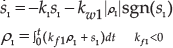
\begin{array}{l} {\dot{s}}_{1} = - k_{1} s_{1} - k_{w 1} | ρ_{1} | sgn (s_{1}) \\ ρ_{1} = \int_{0}^{t} (k_{f 1} ρ_{1} + s_{1}) d t \begin{matrix} k_{f 1} < 0 \end{matrix} \end{array}

(30)

where, k₁ and k_f₁ are the parameters of weighted integral gain reaching law. In the integral item ρ₁, k_f₁ are weighted coefficients, when ρ ₁>0, k_f₁ ρ ₁<0, and when ρ ₁<0, k_f₁ ρ ₁>0, so it can avoid the switch gain increasing effectively when the system states are not in the sliding mode phase and can improve the control performance of the parallel manipulator system.

According to Eq. (29) and (30), the sliding mode controller for the subsystem is designed as follows

\begin{matrix} τ_{1} = b_{​_{1}}^{- 1} [{\overset{..}{y}}_{d} + λ_{1} γ_{1} (e_{1} - z_{1})^{γ_{1} - 1} ({\dot{e}}_{1} - {\dot{z}}_{1}) - f_{1} \dot{y} \\ - d_{1} + k_{1} s_{1} + k_{w 1} | ρ_{1} | sgn (s_{1})] \end{matrix}

(31)

Due to the existence of disturbance d₁, the control law in Eq. (31) cannot be precisely determined. In order to reduce the influence of the unknown perturbations and improve system stability, we adopt the adaptation laws to estimate the external disturbance online. Here, define d̂₁ as the estimation of d₁. So, Eq. (31) can be rewritten as follows

\begin{matrix} τ_{1} = b_{​_{1}}^{- 1} [{\overset{..}{y}}_{d} + λ_{1} γ_{1} (e_{1} - z_{1})^{γ_{1} - 1} ({\dot{e}}_{1} - {\dot{z}}_{1}) - f_{1} \dot{y} \\ - {\hat{d}}_{1} + k_{1} s_{1} + k_{w 1} | ρ_{1} | sgn (s_{1})] \end{matrix}

(32)

Similarly, the control laws for other subsystems are designed as

\begin{array}{l} τ_{2} = b_{​_{2}}^{- 1} [{\overset{..}{z}}_{d} + λ_{2} γ_{2} (e_{2} - z_{2})^{γ_{2} - 1} ({\dot{e}}_{2} - {\dot{z}}_{2}) - f_{2} \dot{z} \\ - {\hat{d}}_{2} + k_{2} s_{2} + k_{w 2} | ρ_{​_{2}} | sgn (s_{2})] sgn (s_{2})] \end{array}

(33)

\begin{array}{l} τ_{3} = b_{​_{3}}^{- 1} [{\overset{..}{β}}_{d} + λ_{3} γ_{3} e_{3} ​^{γ_{3} - 1} {\dot{e}}_{3} - f_{3} \dot{β} - {\hat{d}}_{3} + k_{3} s_{3} \\ + k_{w 3} | ρ_{​_{3}} | sgn (s_{3})] \end{array}

(34)

4.3 Design of compensator based on RBF neural network

It is noted that the control laws shown in Eqs. (32)∼(34) are designed without considering the coupling force and gravity, and this will greatly reduce the control precision of the system. Here, the coupling force and gravity will be taken into account by compensating to ensure control precision while greatly increase the processing speed. The compensatory model $τ_{c} = {[τ_{c 1}, τ_{c 2}, τ_{c 3}]}^{T}$ is denoted as follows.

τ_{c} = τ_{c c} + G

(35)

It is clear that such a compensatory model is much more complex and time-consuming, especially in the case of high-speed machining, as the RBF neural network is of a simple structure and global optimum convergence performance and is usually used to approximate continuous functions. Here, we design a compensator based on RBF NN to compensate for the cross-coupling force and gravity. The RBF architecture is shown in Figure 4, which has one input layer, one output layer and one hidden layer with variable neuron numbers.

Figure 4.

Structure of RBF NN for compensation of driving forces

The input vector corresponds to the pose variables of the end-effector denoted as X=[x₁, x₂,…,x₉]^T= [y, z, β, ẏ, ż, β,ÿ, z̈, β]^T. On the other hand, the output vector corresponds to the compensation of driving forces in generalized coordinates, denoted as Y = [y₁, y₂, y₃]^T = [τ_c1,τ_c2,τ_c3]^T. The activation function H =[h₁, h₂,…h_m]^T is chosen as a Gaussian function as follows, with

h_{i} = \exp (- \frac{‖ X - C_{i} ‖}{2 σ_{i}^{2}}) \begin{matrix} i = 1, 2, \end{matrix} \dots m

where C_j and σ _j are the centre and width of the ith kernel unit, respectively.

Then, the output of the RBF NN can be expressed as

y_{j} = \sum_{i = 1}^{m} ω_{j i} h_{i} \begin{matrix} \begin{matrix} i = 1, 2, \end{matrix} \dots 3 \end{matrix}

(36)

where ω_ji is the connection weight.

According to the moving characters of the end-effector for the parallel manipulator, the pose dates $X_{i} = {[y_{i}, z_{i}, β_{i}, {\dot{y}}_{i}, {\dot{z}}_{i}, {\dot{β}}_{i}, {\overset{..}{y}}_{i}, {\overset{..}{z}}_{i}, {\overset{..}{β}}_{i}]}^{T}$ (i =1, 2…3000) are reasonably selected in the reachable workspace, and the corresponding compensation of driving force $Y_{i} = {[τ_{c 1 i}, τ_{c 2 i}, τ_{c 3 i}]}^{T}$ can be computed through Eq. (36); then, all of the dates are normalized in the range of [0, 1] and the training samples are obtained. Choose 70% of the samples to train the RBF neural networks offline and the remaining data are used to validate the quality of the network. In actual control conditions, the compensations of the driving force can be obtained online using the trained neural network.

Considering the coupling force and gravity, the control law can be expressed as

τ^{'} = τ + {\hat{τ}}_{c}

Where, ${\hat{τ}}_{c} = {[{\hat{τ}}_{c 1}, {\hat{τ}}_{c 2}, {\hat{τ}}_{c 2}]}^{T}$ is the estimate of the RBF neural network, as follows

{\hat{τ}}_{c} = {\hat{W}}^{T} H

(37)

Proof: consider a Lyapunov function candidate as follows

V = \frac{1}{2} s^{T} M's + \frac{1}{2 σ_{i}} \sum_{i = 1}^{3} {\tilde{d}}_{i} ​^{2} + \frac{1}{2} t r ({\tilde{W}}^{T} Γ^{- 1} \tilde{W})

(38)

Where, d˜_i is the estimation error of adaptation laws, denoted as d˜_i = d_i* − d̂_i, and W˜ is the error between the optimal value W* and the estimated value Ŵ of the RBFNN

The derivative of V is computed as follows

\begin{array}{l} \dot{V} = s^{T} (M' \dot{s} + \frac{1}{2} \dot{M}' s) - \sum_{i = 1}^{3} {\tilde{d}}_{i} {\hat{d}}_{i} / σ_{i} + \frac{1}{2} tr ({\tilde{W}}^{T} Γ^{- 1} \dot{\tilde{W}}) \\ = s^{T} (M' \dot{s} + C' s) + \frac{1}{2} s^{T} (\dot{M}' - 2 C') s - \sum_{i = 1}^{3} {\tilde{d}}_{i} {\hat{d}}_{i} / σ_{i} + \frac{1}{2} tr ({\tilde{W}}^{T} Γ^{- 1} \dot{\tilde{W}}) \end{array}

Taking into account the property of the dynamic model of the parallel manipulator, we have s^T(Ṁ′−2C′)s=0; then, the derivative of Lyapunov function is expressed as follows

\begin{matrix} \dot{V} = s^{T} (M' \dot{s} + C' s) - \sum_{i = 1}^{3} {\tilde{d}}_{i} {\hat{d}}_{i} / σ_{i} + \frac{1}{2} tr ({\tilde{W}}^{T} Γ^{- 1} \dot{\tilde{W}}) \\ = s^{T} [\begin{array}{l} C_{11} ({\dot{e}}_{1} + λ_{1} (e_{1} - z_{1})^{γ_{1}}) + M_{11} ({\overset{..}{e}}_{1} + λ_{1} γ_{1} (e_{1} - z_{1})^{γ_{1} - 1} ({\dot{e}}_{1} - {\dot{z}}_{1})) \\ C_{22} ({\dot{e}}_{2} + λ_{2} (e_{2} - z_{2})^{γ_{2}}) + M_{22} ({\overset{..}{e}}_{2} + λ_{2} γ_{2} (e_{2} - z_{2})^{γ_{2} - 1} ({\dot{e}}_{2} - {\dot{z}}_{2})) \\ C_{33} ({\dot{e}}_{3} + λ_{3} e_{3} ​^{γ_{3}}) + M_{33} ({\overset{..}{e}}_{3} + λ_{3} γ_{3} e_{3} ​^{γ_{3} - 1} {\dot{e}}_{3}) \end{array}] - \sum_{i = 1}^{3} {\tilde{d}}_{i} {\hat{d}}_{i} / σ_{i} + \frac{1}{2} tr ({\tilde{W}}^{T} Γ^{- 1} \dot{\tilde{W}}) \\ = s^{T} [\begin{matrix} C_{11} ({\dot{e}}_{1} + λ_{1} (e_{1} - z_{1})^{γ_{1}}) + M_{11} ({\overset{..}{y}}_{d} - \overset{..}{y} + λ_{1} γ_{1} (e_{1} - z_{1})^{γ_{1} - 1} ({\dot{e}}_{1} - {\dot{z}}_{1})) \\ C_{22} ({\dot{e}}_{2} + λ_{2} (e_{2} - z_{2})^{γ_{2}}) + M_{22} ({\overset{..}{z}}_{d} - \overset{..}{z} + λ_{2} γ_{2} (e_{2} - z_{2})^{γ_{2} - 1} ({\dot{e}}_{2} - {\dot{z}}_{2})) \\ C_{33} ({\dot{e}}_{3} + λ_{3} e_{3} ​^{γ_{3}}) + M_{33} ({\overset{..}{β}}_{d} - \overset{..}{β} + λ_{3} γ_{3} e_{3} ​^{γ_{3} - 1} {\dot{e}}_{3}) \end{matrix}] - \sum_{i = 1}^{3} {\tilde{d}}_{i} {\hat{d}}_{i} / σ_{i} + \frac{1}{2} tr ({\tilde{W}}^{T} Γ^{- 1} \dot{\tilde{W}}) \\ = s^{T} [\begin{array}{l} C_{11} ({\dot{e}}_{1} + λ_{1} (e_{1} - z_{1})^{γ_{1}}) + M_{11} {\overset{..}{y}}_{d} - (τ_{1} + {\hat{τ}}_{c 1} - C_{11} \dot{y} - G_{1}) + λ_{1} γ_{1} (e_{1} - z_{1})^{γ_{1} - 1} ({\dot{e}}_{1} - {\dot{z}}_{1})) \\ C_{22} ({\dot{e}}_{2} + λ_{2} (e_{2} - z_{2})^{γ_{2}}) + M_{22} {\overset{..}{z}}_{d} - (τ_{2} + {\hat{τ}}_{c 2} - C_{22} \dot{z} - G_{2}) + λ_{2} γ_{2} (e_{2} - z_{2})^{γ_{2} - 1} ({\dot{e}}_{2} - {\dot{z}}_{2})) \\ C_{33} ({\dot{e}}_{3} + λ_{3} e_{3} ​^{γ_{3}}) + M_{33} {\overset{..}{β}}_{d} - (τ_{3} + {\hat{τ}}_{c 3} - C_{33} \dot{β} - G_{3}) + λ_{3} γ_{3} e_{3} ​^{γ_{3} - 1} {\dot{e}}_{3}) \end{array}] - \sum_{i = 1}^{3} {\tilde{d}}_{i} {\hat{d}}_{i} / σ_{i} + \frac{1}{2} tr ({\tilde{W}}^{T} Γ^{- 1} \dot{\tilde{W}}) \end{matrix}

(39)

Considering the characteristics of the parallel manipulator, choose $\dot{\tilde{W}} = - Γ H s^{T}$ , then $\dot{\hat{W}} = Γ H s^{T}$ . The adaptation law is chosen as ${\dot{\hat{d}}}_{i} = - σ_{i} s_{i}$ . Moreover, the convergence errors of outputs for the adaptation law and RBFNN are assumed to be zero.

By substituting (31) ∼ (34) and (37) into (39), one can obtain

\begin{matrix} \dot{V} = s^{T} [\begin{matrix} - k_{1} s_{1} - k_{w 1} | ρ_{1} | sgn (s_{1}) \\ - k_{2} s_{2} - k_{w 2} | ρ_{2} | sgn (s_{2}) \\ - k_{3} s_{3} - k_{w 3} | ρ_{3} | sgn (s_{3}) \end{matrix}] \\ = - \sum_{i = 1}^{3} (k_{i} s_{i} ​^{2} + k_{w i} | ρ_{i} | | s_{i} |) \leq 0 \end{matrix}

(40)

Thus, the proposed sliding mode controller can guarantee the stability of the closed loop control system. Moreover, when the subsystem A is in the terminal sliding mode (s ₁=0), we have e₁=z₁, ė ₁=0. It follows from (27a) that ė₁=0 only if z ₁=0, which implies that s₂=0. Meanwhile, when s₂=0, we have e₂=z₂, ė₂=0; it follows from (27b) that ė₂=0, only if z₂ = 0, which implies that s₃ = 0, ė₃ = 0, that is y = y_d, z = z_d, β=β_d. Therefore, it can be concluded that the stabilization of each subsystem can be achieved and the actual pose of the end-effector for the parallel manipulator can track the desired one in finite time.

5. Simulation results

In order to verify the control performances of the proposed controller (DNTSMC), an intensive series of simulation studies has been fulfilled on the 3-DOF parallel manipulator. The mechanism parameters are given as follows: m=8.103kg, m_b1=m_b2=11.815kg, m_b3=16.401kg, m_l1=m_l2=10.875kg, m_l3=8.525kg, m_b4=70.318kg, L₁=L₂=269mm, r ₁=r ₂=98.17mm, r₃=140mm, R₁=R₂=213.91mm, R₃=207.8mm, L₃=216mm, and parameters for the proposed controller are designed as λ _i=30, γ_i=9/7, Φ_z1=Φ_z2=0.005, Z_u1=Z_u2=0.9, k_i=500, k_w=20, c_i=0.06rand(2,5) and σ _i=15 with i=1,2,3.

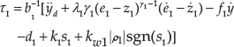
Considering the workspace and singularities of the parallel manipulator, the moving platform is required to move along a circular path with the initial pose (0.015m, 0.035mm, 0.518rad), the desired trajectory is chosen to be y =0.05sin(0.5π*t), z=0.05cos(0.5πt), β=π/6 and the external disturbances are assumed as t_di=0.005randn(1,1) with i=1,2,3 and the simulation results are shown in Figures 5 –8.

Figure 5.

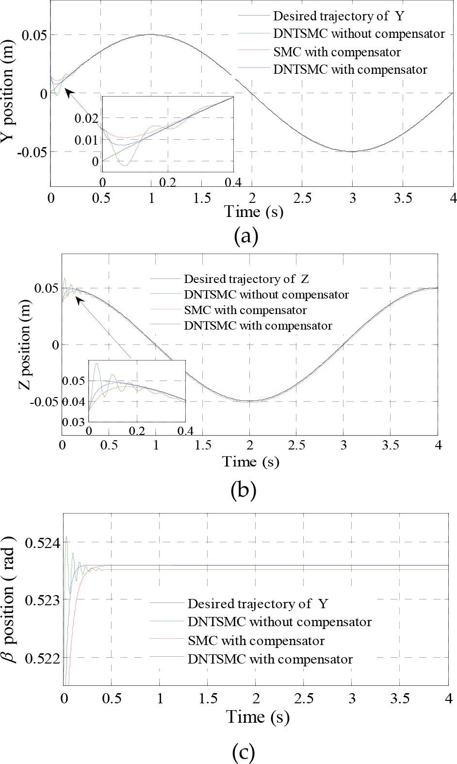
Tracking results in Y, Z and β direction

Figure 6.

Tracking errors in Y, Z and β direction

Figure 7.

Driving forces

Figure 8.

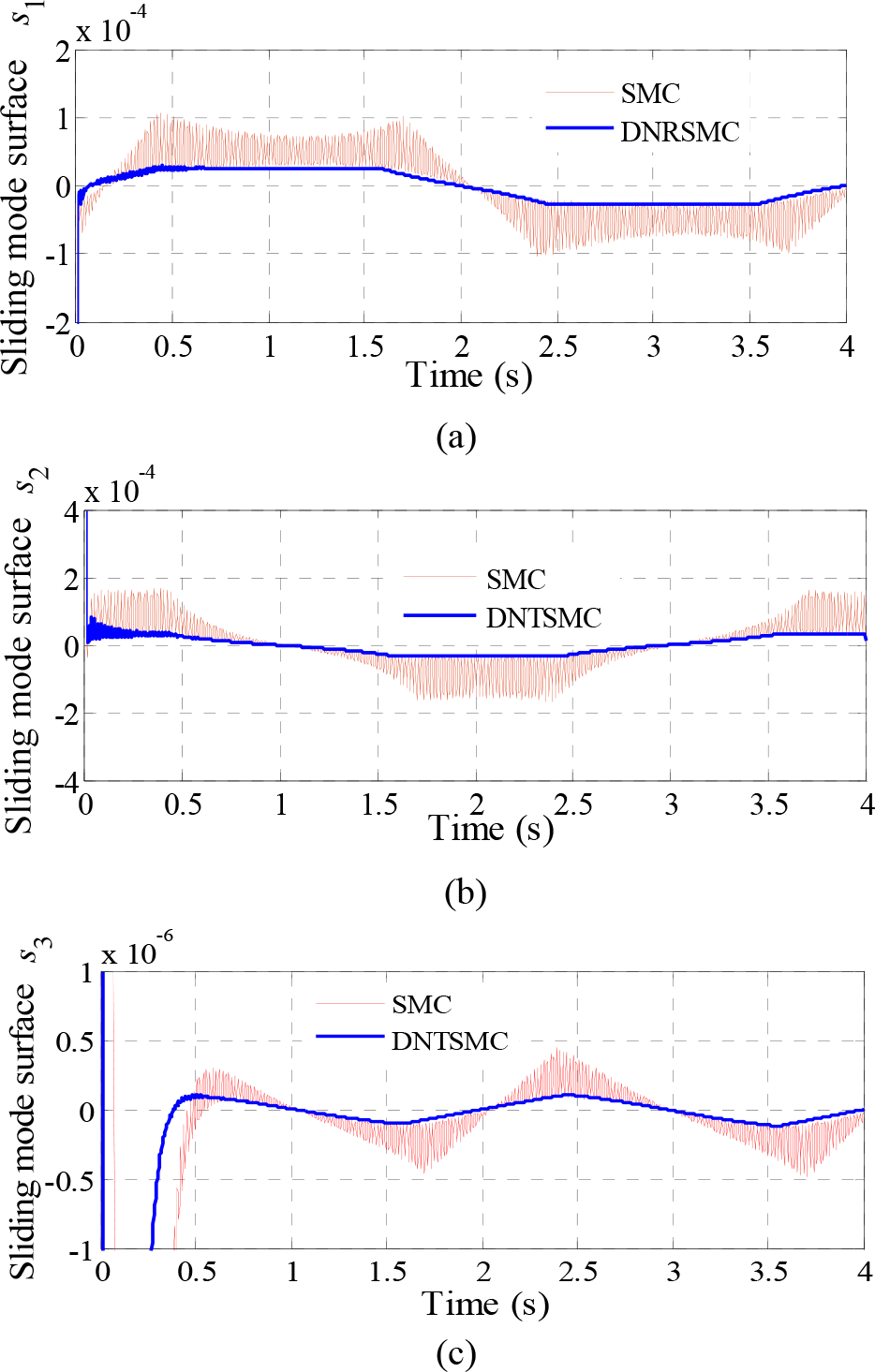
Sliding mode surfaces

The actual trajectory tracking results in the Y, Z and β direction, and the corresponding tracking errors are shown in Figure 5 and Figure 6, respectively; it can be seen that the proposed DNTSMC with compensator based on RBF NN enables the end-effector of the parallel manipulator to precisely follow the desired trajectory, and achieves higher precision than the controller without the compensator. Moreover, compared with the conventional sliding mode control, the proposed DNTSMC has a faster dynamic response. As can be deduced that the proposed control method shows excellent tracking performances such as a faster response, and smaller overshoot and tracking precision than the other controllers along all DOFs.

In this case, the driving forces of the four joints are shown in Figure 7. It is observed from Figure 7 and the magnified picture that the driving forces of the proposed control operate without significant control chatter. Moreover, it is clear that the maximum amplitude for the driving forces is approximately a quarter of that of the controller without the compensator, so the energy consumption can be greatly deduced. Furthermore, it is observed from Figure 8 that the sliding mode surfaces are smoother than those of the conventional sliding mode control because a negative weighted value Kf is introduced in the approaching phase, which can reduce the switching gain greatly; therefore, it can minimize chattering significantly. Additionally, the driving force and sliding mode surface curves shall actually be sinusoidal waveform, which are determined by the symmetry of the mechanism structure and the trajectory for the parallel manipulator end-effector.

6. Experimental results

The proposed control was experimentally evaluated using the 3-DOF parallel manipulator, as shown in Figure 9.

Figure 9.

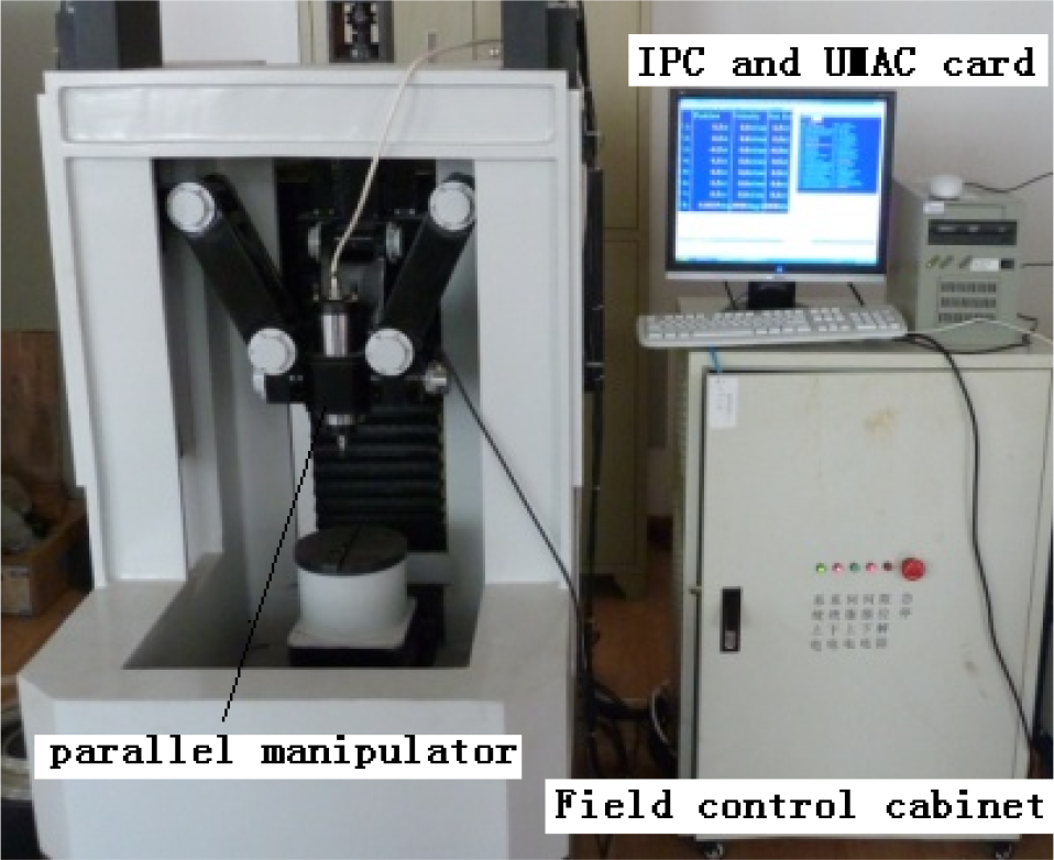
Experiment setup

The test setup is composed of a 3-DOF parallel manipulator, a real-time industrial computer, a Delta Tau UMAC, four Mitsubishi Electric servo systems and a binocular vision positioning system [26,28]. Moreover, during physical implementation, shift registers with a proper initial value are adopted to remove the algebraic loop caused by acceleration feedback.

Supposing the desired moving trajectory for the end-effector is a square with side length 60mm with the centre of (0, −90mm) in the YZ plane under the initial point (0, 30mm, −90mm). The maximum translational speed and angular velocity in the Y, Z direction are set to 6m/min and 12°/s, respectively, and the maximum acceleration for every drive is 1g. Choose spatial coordinates (−80mm, 0mm, −200mm) as the test point for the binocular vision positioning system and select 16 test points p_i (i=1,2…16) as the trajectory test points on the desired trajectory. Repeat the same work 20 times in a counter clockwise direction and choose the average value as the qualitative pose data, as shown in table 1. As can be seen, the maximal tracking errors in Y, Z, β directions are 0.67mm, 0.52mm and 0.24°, respectively, under the proposed decoupled nonsingular terminal sliding mode controller. The maximal tracking errors in all DOFs are 0.85mm, 0.99mm and 0.33°. Moreover, the time to run the whole control program once is 360ms; as a result, the proposed decoupled nonsingular terminal sliding mode controller can satisfy control precision and real-time application for the 3-DOF redundantly actuated parallel manipulator system.

Table 1.

Test result

Test point	Desired Value			SMC			DNTSMC
Test point	y_d (mm)	z_d (mm)	β_d (°)	y′(mm)	z′(mm)	β′(°)	y(mm)	z(mm)	β(°)
P₁	40.00	−90.00	0	40.16	−90.53	0.07	40.02	−90.32	0.06
P₂	40.00	−70.00	0	40.34	−69.80	0.16	40.28	−69.67	0.12
P₃	40.00	−50.00	0	39.62	−50.64	−0.35	39.78	−50.42	−0.23
P₄	20.00	−50.00	0	19.89	−49.14	−0.14	19.82	−49.20	−0.10
P₅	0.00	−50.00	0	0.14	−49.68	−0.19	0.03	−49.78	−0.21
P₆	−20.00	−50.00	0	−20.45	−49.78	−0.97	−20.33	−49.69	0.02
P₇	−40.00	−50.00	0	−39.52	−50.13	−0.15	−39.54	−50.02	−0.11
P₈	−40.00	−70.00	0	−40.85	−69.87	0.30	−40.52	−69.66	0.22
P₉	−40.00	−90.00	0	−40.36	−90.65	0.03	−40.23	−90.52	0.03
P₁₀	−40.00	−110.00	0	−38.98	−110.44	0.02	−39.78	−110.36	−0.01
P₁₁	−40.00	−130.00	0	−39.64	−129.35	0.25	−39.42	−129.65	0.21
P₁₂	−20.00	−130.00	0	−20.50	−129.69	−0.16	−20.36	−129.78	−0.13
P₁₃	0.00	−130.00	0	0.39	−130.78	0.02	0.42	−130.52	0.02
P₁₄	20.00	−130.00	0	20.74	−130.64	−0.33	20.39	−130.34	−0.23
P₁₅	40.00	−130.00	0	39.66	−130.99	−0.16	39.87	−130.48	−0.12
P₁₆	40.00	−110.00	0	40.12	−109.65	−0.22	39.42	−109.78	−0.24

7. Conclusions

In this paper, a decoupled nonsingular terminal sliding mode controller with cross-coupling and gravity compensation is addressed to improve the control performance for a novel 3-DOF parallel manipulator with actuation redundancy. The inverse dynamic model for a novel 3-DOF redundantly actuated parallel manipulator is formulated in the task space using Lagrangian formalism and decoupled into three entirely independent subsystems under generalized coordinates to significantly reduce system complexity. Then, the nonsingular terminal sliding mode controllers are designed to drive the subsystem states to original equilibrium points simultaneously by two intermediate variables in finite time, and the stability is proved by utilizing Lyapunov theory. Additionally, a RBF neural network is used to compensate for the cross-coupling force and gravity to enhance the control precision. Simulation and experimental results show that the proposed method is of excellent control performance with a fast response, high precision and strong robustness.

Footnotes

8. Acknowledgements

This work was financially supported by National Natural Science Foundation of China (Grant No. 51375210), the Priority Academic Program Development of Jiangsu Higher Education Institutions, Zhenjiang Municipal Industry Key Technology R&D Program (Grant No. GY2013062) and Jiangsu University Senior Professionals Scientific Research Foundation (No. 13JDG047).

References

Noshadi

Mailah

Zolfagharian

(2011) Intelligent active force control of a 3-RRR parallel manipulator incorporating fuzzy resolved acceleration control. Applied Mathematical Modelling, j. 36(6): 2370–2383.

Qin

Y. D.

Shirinzadeh

B.J.

Tian

Y.L.

. (2013) Design issues in a decoupled XY stage: Static and dynamics modeling, hysteresis compensation, and tracking control. Sensors and Actuators A: Physical, j. 194: 95–105.

T. M.

Wang

J. S.

. (2013) Stiffness and natural frequency of a 3-DOF parallel manipulator with consideration of additional leg candidates. Robotics and Autonomous Systems, j. 61(8): 868–875.

Weng

C. C.

W. S.

(2010) H8 tracking adaptive fuzzy integral sliding mode control for parallel manipulators. IEEE International Conference on Systems, Man and Cybernetics, Taipei, Taiwan: 4197–4204.

Yang

C. F.

Huang

Q. T.

Han

J. W.

(2012) Decoupling control for spatial six-degree-of-freedom electro-hydraulic parallel robot. Robotics and Computer-Integrated Manufacturing, j. 28(1): 14–23.

Briot

Arakelian

Guegan

Pamins

(2012) A new family of partially decoupled parallel manipulators. Mechanism and Machine Theory, j. 44(2): 425–444.

Legnani

Fassi

Giberti

. (2012) A new isotropic and decoupled 6-DOF parallel manipulator. Mechanism and Machine Theory, j. 58:64–81.

Yang

C. F.

Huang

Q. T.

Jiang

H. Z.

. (2010) PD control with gravity compensation for hydraulic 6-DOF parallel manipulator. Mechanism and Machine Theory, j. 45 (4): 666–677.

Liu

Y. B.

Han

X. Y.

Zhao

X. H.

(2009) Decoupled control of a 3-RRRT parallel robot. Journal of Harbin Institute of Technology, j. 41(12): 247–249 (In Chinese).

10.

Duchaine

Bouchard

Gosselin

C. M.

(2007) Computationally efficient predictive robot control. IEEE/ASME Transactions on Mechatronics, j. 12(5): 570–578.

11.

Bayramoglu

Komurcugil

(2013) Nonsingular decoupled terminal sliding-mode control for a class of fourth-order nonlinear systems. Communications in Nonlinear Science and Numerical Simulation, j. 18(9): 2527–2539.

12.

Fei

(2013) Adaptive sliding mode vibration control

13.

D. S.

Guo

H. B.

(2007) Adaptive sliding control of six-DOF flight simulator motion platform. Chinese Journal of Aeronautics, j. 20(5): 425–433.

14.

Achili

Daachi

Ali-Cherif

. (2009) Combined multi-layer perceptron neural network and sliding mode technique for parallel robots control: An adaptive approach. Proceedings of International Joint Conference on Neural Networks, IEEE, Atlanta, United states: 28–35.

15.

Gao

G. Q.

Luo

Liu

X. J.

. (2010) Chattering-free sliding mode control for the parallel mechanism of a virtual axis mechanism tool. Proceedings of the 29th Chinese Control Conference, CCC'10, IEEE, Beijing, China: 5670–5675.

16.

Gao

G. Q.

Xia

W. J.

Song

(2011) The application of the adaptive sliding mode control with an integral-operation switching surface in the parallel robot. Proceedings of the 2011 IEEE International Conference on Computer Science and Automation Engineering, CSAE 2011, IEEE, Shanghai, China: 302–306.

17.

Bayramoglu

Komurcugil

(2013) Nonsingular decoupled terminal sliding-mode control for a class of fourth-order nonlinear systems. Communications in Nonlinear Science and Numerical Simulation, j. 18(9): 2527–2539.

18.

Zak

(1998) Terminal attractors for addressable memory in neural network. Physics Letters A, j. 133(1,2):18–22.

19.

Man

Z. H.

Paplinski

A. P.

H. R.

(1994) A robust MIMO terminal sliding mode control scheme for rigid robotic manipulators. IEEE Transactions on Automatic Control, j. 39(12): 2464–2469.

20.

T. H. S.

Huang

Y. C.

(2010) MIMO adaptive fuzzy terminal sliding-mode controller for robotic manipulators. Information Sciences, j. 180 (23): 4641–4660.

21.

Hasan

(2012) Adaptive terminal sliding-mode control strategy for DC–DC buck converters. ISA Transactions, j. 51(6): 673–681.

22.

Feng

X. H.

Man

Z. H.

, (2002) Non-singular terminal sliding mode control of rigid manipulators. Automatica, j. 38(12): 2159–2167.

23.

Yang

S. H.

J. Y.

X. H.

, (2012) Continuous nonsingular terminal sliding mode control for systems with mismatched disturbances. Automatica, j. 49 (7): 2287–2291.

24.

Liu

X. J.

Wang

J. S.

Xie

F. G.

(2010) A multi-axis synchronous hybrid mechanism, China. Patent ZL 200810113768.4.

25.

Xie

F. G.

Liu

X. J.

Wang

J. S.

(2012) A 3-DOF parallel manufacturing module and its kinematic optimization. Robotics and Computer-Integrated Manufacturing, j. 28(3): 334–343.

26.

Niu

X. M.

Gao

G. Q.

Liu

X. J.

. (2013) Dynamics and control of a novel 3-DOF parallel manipulator with actuation redundancy. International Journal of Automation and Computing, j. 10 (6): 552–562.

27.

Wang

L. P.

Wang

J. S.

, (2010) Dynamic formulation of a planar 3-DOF parallel manipulator with actuation redundancy. Robotics and Computer-Integrated Manufacturing, j. 26(1): 67–73.

28.

Niu

X. M.

Gao

G. Q.

Liu

X. J.

. (2013) Dynamics modeling and experiments of 3-DOF parallel mechanism with actuation redundancy. Nongye Gongcheng Xuebao/Transactions of the Chinese Society of Agricultural Engineering, j.29(16): 31–41.

29.

Wang

J. S.

Wang

L. P.

. (2009) Dynamic formulation of redundant and nonredundant parallel mechanisms for dynamic parameter identification. Mechatronics, j. 19(4): 586–590.

30.

Yorgancioglu

Komurcugil

(2010) Decoupled sliding-mode controller based on time-varying sliding surfaces for fourth-order systems. Expert Systems with Applications, j. 37(10): 6764–6774.

31.

Bayramoglu

Komurcugil

(2013) Nonsingular decoupled terminal sliding-mode control for a class of fourth-order nonlinear systems. Communications in Nonlinear Science and Numerical Simulation, j. 18 (9): 2527–2539.

32.

Javadi

M. J.

Madani

(2011) A decoupled adaptive neuro-fuzzy sliding mode control system to control rotating stall and surge in axial compressors. Expert Systems with Applications, j. 38 (4): 4490–4496.

33.

Feng

X. H.

Man

Z. H.

(2002) Non-singular terminal sliding mode control of rigid manipulators. Automatica, j. 38 (12): 2159–2167.

Decoupled Sliding Mode Control for a Novel 3-DOF Parallel Manipulator with Actuation Redundancy

Abstract

Keywords

1. Introduction

2. Model of parallel manipulator

2.1 Structure description

2.2 Inverse kinematics analysis

3. Dynamic modelling

3.1 Kinetic energy

3.2 Potential energy

3.3 Dynamic formulation

4. Controller design

4.1 Control strategy

4.2 Design of nonsingular terminal sliding mode control

4.3 Design of compensator based on RBF neural network

5. Simulation results

6. Experimental results

7. Conclusions

Footnotes

8. Acknowledgements

References