Sage Journals: Discover world-class research

Abstract

The simulation of robot systems is becoming very popular, especially with the lowering of the cost of computers, and it can be used for layout evaluation, feasibility studies, presentations with animation and off-line programming.

The trajectory planning of redundant manipulators is a very active area since many tasks require special characteristics to be satisfied. The importance of redundant manipulators has increased over the last two decades because of the possibility of avoiding singularities as well as obstacles within the course of motion. The angle that the last link of a 2 DOF manipulator makes with the x-axis is required in order to find the solution for the inverse kinematics problem. This angle could be optimized with respect to a given specified key factor (time, velocity, torques) while the end-effector performs a chosen trajectory (i.e., avoiding an obstacle) in the task space.

Modeling and simulation of robots could be achieved using either of the following models: the geometrical model (positions, postures), the kinematic model and the dynamic model.

To do so, the modelization of a 2-R robot type is implemented. Our main tasks are comparing two robot postures with the same trajectory (path) and for the same length of time, and establishing a computing code to obtain the kinematic and dynamic parameters.

SolidWorks and MATLAB/Simulink softwares are used to check the theory and the robot motion simulation.

This could be easily generalized to a 3-R robot and possibly therefore to any serial robot (Scara, Puma, etc.).

The verification of the obtained results by both softwares allows us to qualitatively evaluate and underline the validityof the chosen model and obtain the right conclusions. The results of the simulations are discussed and an agreement between the two softwares is certainly obtained.

Keywords

Multibody Systems 2-R Robot Modelization Kinematic Model Dynamic Behaviour Manipulability Simulation

1. Introduction

Robotics is a special engineering science which deals with robot design, modelling, controlling and utilization. Nowadays robots accompany people in everyday life and have taken over some of their daily procedures. The range of robot utilization is very wide, from toys through to office and industrial robots, through to very sophisticated ones needed for space exploration.

A large family of robot manufacturing equipment exists, supplying the motion required in manufacturing processes such as arc welding, spray painting, assembly, pick and place, cutting, polishing, milling, drilling, etc. Of this class of equipment, an increasingly popular type is the industrial robot. Different manipulator configurations are available such as rectangular, cylindrical, spherical, revolute and horizontal jointed.

Kinematically redundant manipulators have many advantages over non-redundant robots. A redundant manipulator is defined as having an infinite number of solutions to the joint variables of the manipulator for a given task. It can avoid obstacles and singularities, and is an excellent candidate for optimization techniques. Many optimization techniques have been applied to select the optimal trajectory of a manipulator using different criteria such as minimum time, minimum kinetic energy and obstacle avoidance.

A manipulation task is usually given in terms of a desired end-effector trajectory. Since the manipulator is controlled by joint servos, a mapping from the task space to the joint space is required. Trajectory planning converts a description of a desired motion to a trajectory defining the time sequence of intermediate configurations of the arm between the origin and the final destination. An effective approach to the motion control problem for robotic manipulators is the so-called kinematic control.

This is based on an inverse kinematic transformation which feeds the reference values corresponding to an assigned end-effector trajectory to the joint servos.

A vertical revolute configuration, a 2-R robot with two degrees of freedom is generally well-suited for small parts insertion tasks for assembly lines like electronic components insertion [2]. Although the final aim is real robotics, it is often very useful to perform simulations prior to investigations with real robots [1]. This is because simulations are easier to setup, less expensive, faster and more convenient to use. Building up new robot models and setting up experiments only takes a few hours. A simulated robotics setup is less expensive than real robots and real world setups, thus allowing better design exploration. Simulations often run faster than real robots while all the parameters are easily displayed on screen [3].

The possibility to perform real-time simulations becomes particularly important in the later stages of the design process. The final design can be verified before one embarks on the costly and time consuming process of building a prototype [4].

The need for accurate and computationally efficient manipulator dynamics has been extensively emphasized in recent years. The modelling and simulation of robot systems by using various program softwares will facilitate the process of designing, constructing and inspecting the robots in the real world. A simulation is important for robot programmers in allowing them to evaluate and predict the behaviour of a robot, and in addition to verify and optimize the path planning of the process [5]. Moreover, this will save time and money, and play an important role in the evaluation of manufacturing automation [6]. Being able to simulate opens up a wide range of options, helping to solve many problems creatively. One can investigate, design, visualize and test an object before making it a reality [7].

In this work, a two axis 2-R robot system for a “pick and place” operation will be designed and developed using the SolidWorks program and MATLAB/Simulink simultaneously as shown in Figure 1 and Figure 2.

Figure 1.

A 2-R robot using SolidWorks

Figure 2.

The same 2-R robot modelled in MATLAB/Simulink

The structure will be built depending on the principles of solid bodies' modelling with SD technology [8, 9].

The individual joints' trajectories, velocities and accelerations can be obtained using inverse kinematics equations.

To emphasize the obtained results in the SolidWorks program, simulations using MATLAB/Simulink software will be carried out. The results of both sofwares will be presented and discussed. In the paper, the kinematic equations for a 2-R robot as well as the robot dynamics for each joint were developed using the D-H formulation.

The paper is organized as follows: in chapter 2 forward (direct) kinematics, inverse kinematics as well as the dynamics of the 2R robot are presented. In chapter 3 we present the simulation applications, implementing both softwares, and finally in the concluding chapter 4 some important results are shown.

2. Robot kinematics and dynamics

2.1 Forward kinematics

Consider the two DOF planar redundant manipulator as shown in Figure 3 where the joints' axes are assigned based on the Denavit-Hartenberg representation (Table 1). The manipulator moves in a vertical plane so the gravity force is included in the numerical simulation.

Table 1.

D-H parameters of the 2-R robot

Link	a_i	α _i	d_i	θ_i
1	l ₁	0	0	θ*₁
2	l ₂	0	0	θ*₂

Figure 3.

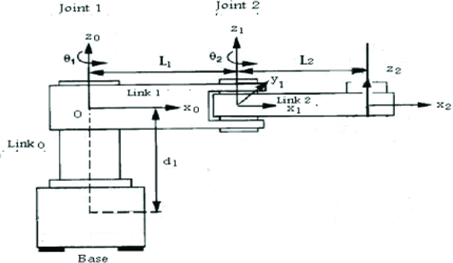
D-H parameters of the two-joint 2-R robot

The (4×4) rigid transformation matrices are:

For the first link:

T_{1}^{0} = [\begin{matrix} c_{1} & - s_{1} & 0 & l_{1} c_{1} \\ s_{1} & c_{1} & 0 & l_{1} s_{1} \\ 0 & 0 & 1 & 0 \\ 0 & 0 & 0 & 1 \end{matrix}]

(1)

and the second link:

T_{2}^{1} = [\begin{matrix} c_{2} & - s_{2} & 0 & l_{2} c_{2} \\ s_{2} & c_{2} & 0 & l_{2} s_{2} \\ 0 & 0 & 1 & 0 \\ 0 & 0 & 0 & 1 \end{matrix}]

(2)

We can then get the overall manipulator transformation matrix:

T_{2}^{0} = [\begin{matrix} c_{12} & - s_{12} & 0 & l_{1} c_{1} + l_{2} c_{12} \\ s_{12} & c_{12} & 0 & l_{1} s_{1} + l_{2} s_{12} \\ 0 & 0 & 1 & 0 \\ 0 & 0 & 0 & 1 \end{matrix}]

(3)

2.2 Inverse kinematics of the robot

The desired location of the 2-R robot is given by the (4×4) matrix:

T_{H}^{R} = (\begin{matrix} n_{X} & o_{X} & a_{X} & p_{X} \\ n_{y} & o_{y} & a_{y} & p_{y} \\ n_{z} & o_{z} & a_{z} & p_{z} \\ 0 & 0 & 0 & 1 \end{matrix})

(4)

For the joint variable θ₂:

The final equation representing the robot is:[10]:

T_{2}^{0} = T_{H}^{R}

(5)

We get:

p_{X} = l_{1} c_{1} + l_{2} c_{12}

(6)

p_{y} = l_{1} s_{1} + l_{2} s_{12}

(7)

We then have:

c_{2} = \frac{1}{2 l_{1} l_{2}} (p_{X} ​_{​}^{2} + p_{y} ​_{​}^{2} - l_{1}^{2} - l_{2}^{2})

(8)

s_{2} = \pm \sqrt{1 - c_{2} ​^{2}}

(9)

θ_{2} = \pm a \tan \frac{s_{2}}{c_{2}}

(10)

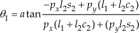
The joint variable θ₁:

Rearranging equation (6) and equation (7) yields:

p_{X} = (l_{1} + l_{2} c_{2}) c_{1} - l_{2} s_{2} s_{1}

(11)

p_{y} = l_{2} s_{2} c_{1} + (l_{1} + l_{2} c_{2}) s_{1}

(12)

Solving equations (11) and (12) by Cramer's rule:

Δ = [\begin{matrix} l_{1} + l_{2} c_{2} & - l_{2} s_{2} \\ l_{2} s_{2} & l_{1} + l_{2} c_{2} \end{matrix}] = {(l_{1} + l_{2} c_{2})}_{​}^{2} + {(l_{2} s_{2})}_{​}^{2}

(13)

and we have:

p_{X}^{2} + p_{y}^{2} = {(l_{1} + l_{2} c_{2})}_{​}^{2} + {(l_{2} s_{2})}_{​}^{2}

(14)

Δ s_{1} = [\begin{matrix} l_{1} + l_{2} c_{2} & p_{x}^{​} \\ l_{2} s_{2} & p_{y}^{​} \end{matrix}]

(15)

Δ c_{1} = [\begin{matrix} p_{x}^{​} & - l_{2} s_{2} \\ p_{y}^{​} & l_{1} + l_{2} c_{2} \end{matrix}]

(16)

s_{1} = \frac{Δ s_{1}}{Δ} = \frac{(l_{1} + l_{2} c_{2}) p_{y}^{​} - l_{2} s_{2} p_{x}^{​}}{p_{X}^{2} + p_{y}^{2}}

(17)

c_{1} = \frac{Δ c_{1}}{Δ} = \frac{(l_{1} + l_{2} c_{2}) p_{x}^{​} + l_{2} s_{2} p_{y}^{​}}{p_{X}^{2} + p_{y}^{2}}

(18)

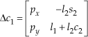
and finally we have:

θ_{1} = a \tan \frac{s_{1}}{c_{1}} = a \tan \frac{(l_{1} + l_{2} c_{2}) p_{y}^{​} \mp l_{2} s_{2} p_{x}^{​}}{(l_{1} + l_{2} c_{2}) p_{x}^{​} \pm l_{2} s_{2} p_{y}^{​}}

(19)

The sign (±) indicates the two postures, “elbow up” and “elbow down”, of the manipulator.

The angles for elbow up are:

θ_{2} = - a \tan \frac{s_{2}}{c_{2}}

(20)

θ_{1} = a \tan \frac{+ p_{x}^{​} l_{2} s_{2} + p_{y}^{​} (l_{1} + l_{2} c_{2})}{p_{x}^{​} (l_{1} + l_{2} c_{2}) - (p_{y}^{​} l_{2} s_{2})}

(21)

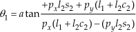
and the angles for elbow down are:

θ_{2} = + a \tan \frac{s_{2}}{c_{2}}

(22)

θ_{1} = a \tan \frac{- p_{x}^{​} l_{2} s_{2} + p_{y}^{​} (l_{1} + l_{2} c_{2})}{p_{x}^{​} (l_{1} + l_{2} c_{2}) + (p_{y}^{​} l_{2} s_{2})}

(23)

Figure 4.

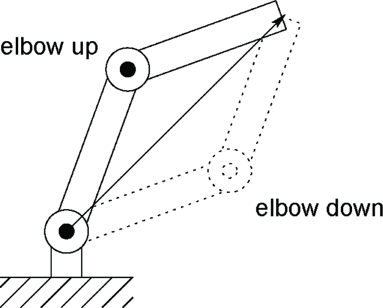
The two postures of the 2-R robot

2.3 Robot dynamics

2.3.1 Kinetic energy

K_{1} = \frac{1}{2} m_{1} l_{1}^{2} {\dot{θ}}_{1}^{2}

(24)

K_{2} = \frac{1}{2} m_{2} l_{1}^{2} {\dot{θ}}_{1}^{2} + \frac{1}{2} m_{2} l_{2}^{2} {({\dot{θ}}_{1}^{​} + {\dot{θ}}_{2}^{​})}_{​}^{2} + m_{2} l_{1}^{​} l_{2}^{​} ({\dot{θ}}_{1}^{2} + {\dot{θ}}_{1}^{​} {\dot{θ}}_{2}^{​}) \cos θ_{2}^{​}

(25)

2.3.2 Potential energy

V_{1} = m_{1} g l_{1}^{​} \sin θ_{1}^{​}

(26)

V_{2} = m_{2} g y_{2}^{​} = m_{2} g [l_{1}^{​} \sin θ_{1}^{​} + l_{2}^{​} \sin (θ_{1}^{​} + θ_{2}^{​})]

(27)

2.3.3 Joints torques

Using the Newton-Euler recursive method we can calculate the necessary torques for each joint:

\begin{array}{l} τ_{1} = m_{2} l_{2}^{2} ({\overset{..}{θ}}_{1}^{​} + {\overset{..}{θ}}_{2}^{​}) + m_{2} l_{1} l_{2} c_{2} (2 {\overset{..}{θ}}_{1}^{​} + {\overset{..}{θ}}_{2}^{​}) \\ + (m_{1} + m_{2}) l_{1}^{2} {\overset{..}{θ}}_{1}^{​} - m_{2} l_{1} l_{2} s_{2} {\dot{θ}}_{2}^{2} - 2 m_{2} l_{1} l_{2} s_{2} {\dot{θ}}_{1}^{​} {\dot{θ}}_{2}^{​} + \\ + m_{2} l_{2} g c_{12} + (m_{1} + m_{2}) l_{1} g c_{1} \end{array}

(28)

τ_{2} = m_{2} l_{1} l_{2} c_{2} {\overset{..}{θ}}_{1}^{​} + m_{2} l_{1} l_{2} s_{2} {\dot{θ}}_{1}^{2} + m_{2} l_{2} g c_{12} + m_{2} l_{2}^{2} ({\overset{..}{θ}}_{1}^{​} + {\overset{..}{θ}}_{2}^{​})

(29)

3. Simulation results

3.1 Application

This application will bear the energetic comparison during the movement of the 2-R robot with m₁ = m₂ = 16.92Kg and l₁ = l₂ = 1m, for the two postures.

We can easily follow and observe the movements of the two postures “elbow down” and “elbow up” for the same nature of the trajectory (path), reaching the same desired position during the same interval of time of 1s as shown in the following diagram:

The initial position (at t = 0) from the homogeneous transformation matrix (3) where θ₁ = 0° and θ₂ = 0° as shown in the following figures:

Starting from a given initial position, i.e.,

p_{X} = 2 ​ ​; ​ ​ p_{y} = 0

To a desired position, i.e,

p_{X} = 0.86 ​ ​; p_{y} = 1.5

The equations of movement for the borrowed path for “elbow down” to reach the desired positions are given by the two following chosen polynomials [11]:

θ_{1} = (10 t_{​}^{4} + 10 t_{​}^{3} + 10 t_{​}^{2}) °

(30)

θ_{2} = (50 t_{​}^{4} + 10 t_{​}^{3}) °

(31)

While the equations of movement for the followed trajectory for “elbow up” to reach the desired position will be given by the relations [11]:

θ_{1} = (60 t_{​}^{4} + 20 t_{​}^{3} + 10 t_{​}^{2}) °

(32)

θ_{2} = (- 50 t_{​}^{4} - 10 t_{​}^{3}) °

(33)

Figure 5.

Link:mass parameters

Figure 6.

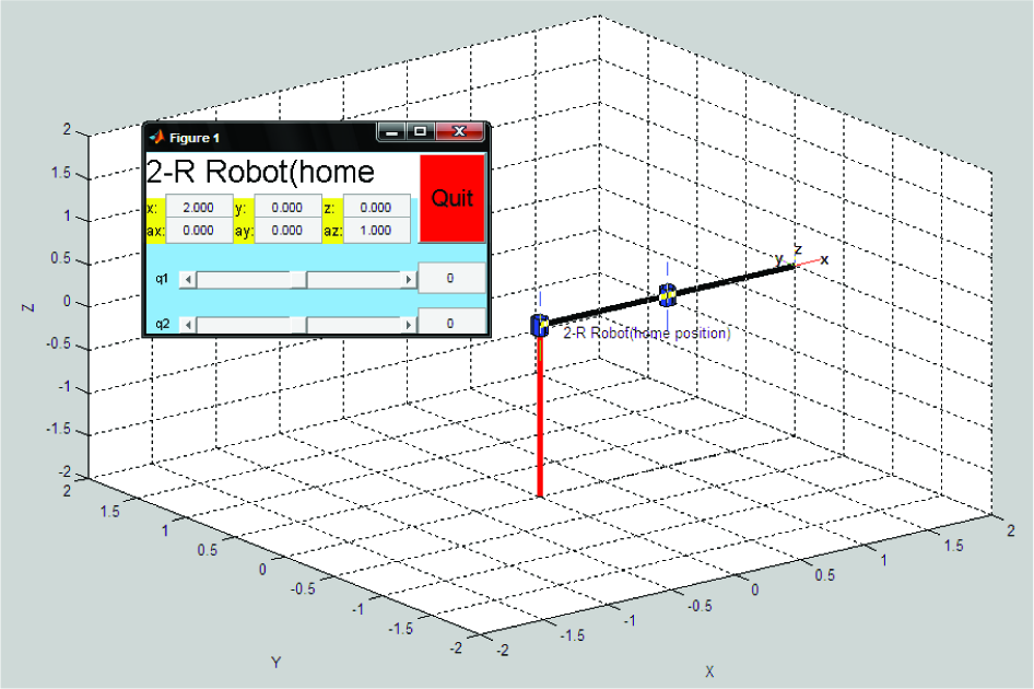
The home position of the 2-R robot (two postures): MATLAB/Simulink

Figure 7.

The home position of the 2-R robot (two postures): SolidWorks

The choice of expressions of θ₁ and θ₂ must satisfy the following two conditions [11]:

In the meantime (interval time) must verify the initial and the desired position.

At every moment the two postures (elbow down and up) must have the same coordinates P_x and P_y.

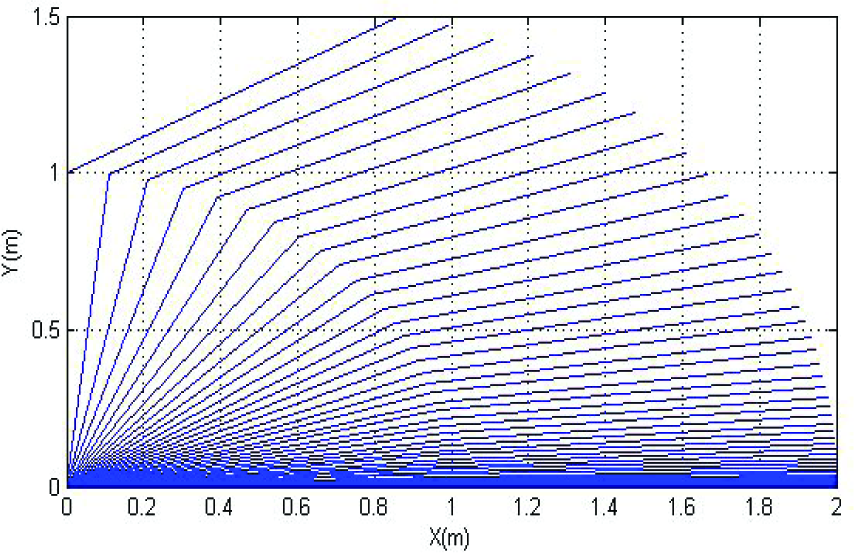
NB: Another example of trajectory generation is given in the Appendix at the end of this paper.

3.1.1 The resulting path

We may check the path:

Applying the relations (20), (21), (22) and (23) in (6) and (7) we can obtain the following table:

3.1.2 Checking the theoretical results of Table 2 using SolidWorks and MATLAB/Simulink

Table 2.

The position for the two postures during 1s

time (sec)	Elbow down				Elbow up
time (sec)	Theta1 (deg)	Theta2 (deg)	p_X (m)	p_y (m)	Theta1 (deg)	Theta2 (deg)	p_X (m)	p_y (m)
0	0	0	2	0	0	0	2	0
0.1	0.11	0.015	1.99	0.004	0.126	−0.015	1.99	0.004
0.2	0.49	0.16	1.99	0.02	0.65	−0.16	1.99	0.02
0.3	1.25	0.67	2	0.05	1.92	−0.67	2	0.05
0.4	2.49	1.92	1.996	0.12	4.41	−1.92	1.996	0.12
0.5	4.37	4.37	1.98	0.21	8.75	−4.37	1.98	0.21
0.6	7.05	8.64	1.95	0.39	15.69	−8.67	1.95	0.39
0.7	10.73	15.43	1.88	0.62	26.16	− 15.43	1.88	0.62
0.8	15.61	25.6	1.71	0.927	41.21	−25.6	1.71	0.927
0.9	20	40.09	1.44	1.20	59.04	−40.09	1.44	1.20
1	30	60	0.86	1.5	90	−60	0.86	1.5

At t=0.5s

Elbow down;

Figure 9.

Elbow down (MATLAB/Simulink)

Figure 10.

Elbow down (SolidWorks)

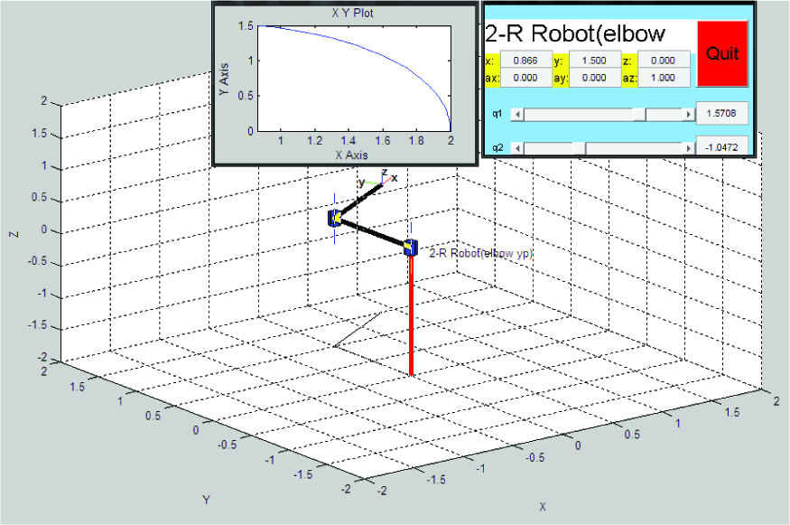
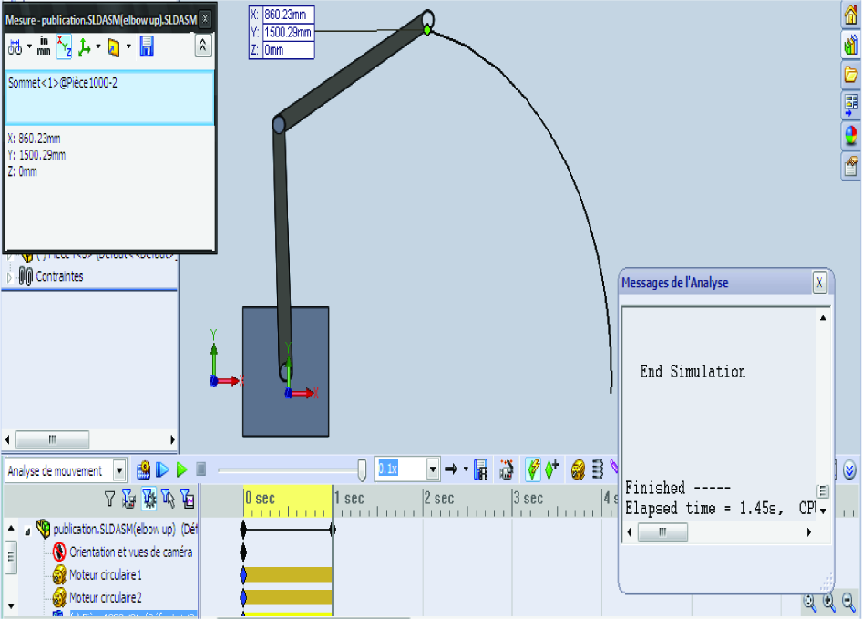
Elbow up:

Figure 11.

Elbow up (MATLAB/Simulink)

Figure 12.

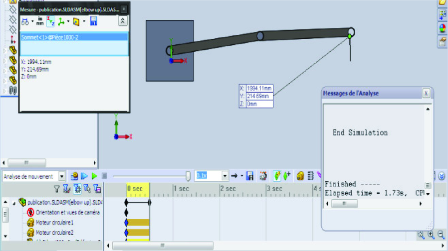
Elbow up (SolidWorks)

and at t=1s

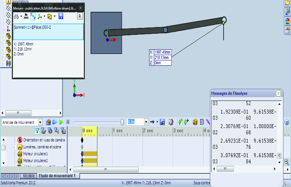
Elbow down;

Figure 13.

Elbow down (MATLAB/Simulink)

Figure 14.

Elbow down (SolidWorks)

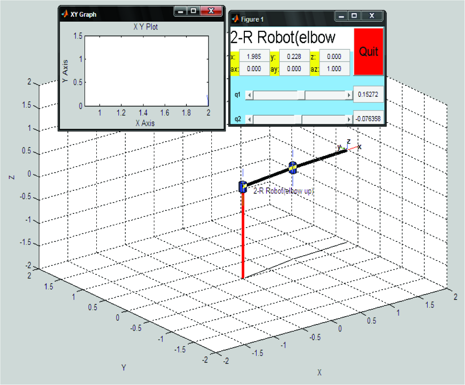
Elbow up;

Figure 15.

Elbow up (MATLAB/Simulink)

The joint variables expressed in MATLAB/Simulink are in radians.

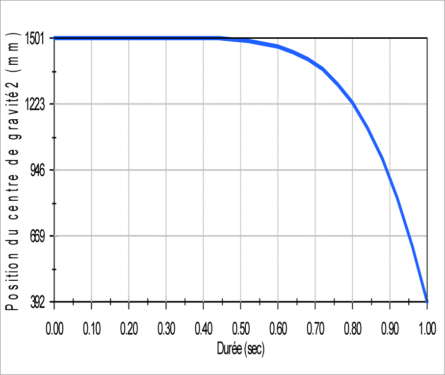
3.1.3 Individual change of position of the two links for the two postures during 1s.

We can take advantage of this analysis using SolidWorks to study the behaviour of the robot for the two postures to establish an energetic balance comparative to these postures.

NOTE 1: The results obtained, whether using SolidWorks or MATLAB/Simulink, are exactly the same. This similarity of results confirms the reliability of the kinematic model.

Figure 16.

Elbow up (SolidWorks)

Figure 17.

Elbow down

Figure 18.

Elbow up

Figure 21.

Link 1(x) elbow up

Figure 22.

link 2(x) elbow up

Figure 23.

Link 1(y) elbow up

Figure 24.

link 2(y) elbow up

Figure 25.

Link 1(x) elbow down

Figure 26.

link 2(x) elbow down

Figure 27.

Link 1(y) elbow down

Figure 28.

Link 2(y) elbow down

Figure 29.

Kinetic energy

NOTE 2: According to the results, we notice that the displacement and velocity of the links 1 and 2 of elbow up are higher than the displacement and velocity of the links 1 and 2 of elbow down, this difference can induce a difference in the consumed energy for the two postures, for the same trajectory and the same desired position.

3.1.5 Simulation of dynamic model

Figure 30.

Potential energy

Figure 31.

Joint torque (1)

Figure 32.

Joint torque (2)

NOTE 3: Comparison between the two postures:

We notice from the simulation results that:

The variation of the total kinetic energy calculated according to posture elbow up is higher than the variation of the total kinetic energy calculated for posture elbow down with: ΔK = 243.02J

The variation of the total potential energy calculated according to posture elbow up is higher than the variation of the total potential energy calculated according to posture elbow down with: ΔV = 82.95J.

We notice also that the torque of joint 1 calculated according to posture elbow up at t=1s is τ₁ = 446.33Nm with a max τ₁ = 900Nm,on the other hand the torque of joint 1 calculated for posture elbow down is τ₁=395.18Nmwith a max τ₁=820Nm

Otherwise the torque of joint 2 calculated according to posture elbow up at t=1s is τ₂ = -127Nm with a max τ₂=300Nm,while the torque of joint 2 calculated according to posture elbow down is τ₂ = 319.65Nm with a max τ₂=330Nm

NOTE 4: The robot consumes much more energy when it is requested to work according to elbow up, for the same trajectory and the same desired position according to elbow down; [10] [11][12]

4. Conclusion

In this paper we used both softwares SolidWorks and MATLAB/Simulink to verify the theory (Table 2) and the simulation of the robot motion.

Checking the results obtained by the two softwares, SolidWorks and MATLAB/Simulink, permitted us to qualitatively develop and highlight the relevance of the studied model.

This can be easily justified when bearing in mind that the effect of different combinations of the two angles will play a major role in determining the value of the potential energy of the second link, and the potential energy of a link will play the greatest role in determining the torque value of that link.

In our case, we can conclude (depending on the obtained results by the comparative analysis of the two postures) that the dissipated energies during the movement of the robot according to the first posture (elbow down) are lower than those which would be dissipated if the robot performs the movement according to the second posture (elbow up), and this is for the same trajectory and the same duration according to the presentations listed above. See notes 1,2,3 and 4.

Footnotes

Appendix

Some trajectories obtained in the displacements of the two postures for the same desired position during 1s:

\begin{array}{l} ​ ​ ​ ​ ​ ​ ​ ​ ​ ​ Elbow up: [11] Elbow down: [11] \\ θ_{1} = {(180 t - 20 t^{2} - 70 t^{5})}^{0} ​ ​ ​ ​ ​ ​ ​ ​ ​ ​ ​ ​ ​ ​ ​ ​ ​ ​ ​ ​ ​ ​ ​ ​ ​ ​ ​ ​ ​ ​ ​ ​ ​ ​ ​ ​ ​ ​ ​ ​ θ_{1} = {(90 t^{10} - 60 t^{2})}^{0} \\ θ_{2} = {(- 180 t + 20 t^{2} + 100 t^{5})}^{0} ​ ​ ​ ​ ​ ​ ​ ​ ​ ​ ​ ​ ​ ​ ​ ​ ​ ​ ​ ​ ​ ​ ​ ​ ​ ​ ​ ​ ​ ​ θ_{2} = {(- 90 t^{10} + 150 t^{2})}^{0} \\ ​ ​ ​ ​ ​ ​ ​ ​ ​ ​ ​ ​ ​ l_{1} = l_{2} = 1 m ​ ​ ​ ​ ​ ​ ​ ​ ​ ​ ​ ​ ​ ​ ​ ​ ​ ​ ​ ​ ​ ​ ​ ​ ​ ​ ​ ​ ​ ​ ​ ​ ​ ​ ​ ​ ​ ​ ​ ​ ​ ​ ​ ​ ​ ​ ​ ​ ​ ​ ​ ​ ​ ​ ​ ​ ​ ​ ​ ​ ​ ​ ​ ​ ​ ​ ​ ​ ​ ​ ​ l_{1} = l_{2} = 1 m \end{array}

References

Sorenti

, 1997. “Efficient Robotic Welding in Shipyards – Virtual Reality Simulation Holds the Key”, Industrial Robot, 24(4), pp.278–281

Das

M.T.

and Dulger

L.C.

, 2005. “Mathematical modelling, simulation and experimental verification of a scara robot”, Simulation Modelling Practice and Theory 13, pp.257–271

Michel

, 2004. “Professional Mobile Robot Simulation”, International Journal of Advanced Robotic Systems, Vol.1, No.1, pp.39–42 ISSN 1729-8806.

Kazi

Merk

Otter

and Fan

, 2002. “Design optimization of industrial robots using the Modelica multi-physics modeling language”, Proceedings of the 33rd ISR (International Symposium on Robotics) October 7 – 11.

Ionescu

Chojnowski

and Constantin

, 2002. “Virtual Reality in Mechanical Engineering, Modelling and Simulation with Solid Dynamics”, ARA-Journal, vol. 2002. No. 27

Ionescu

and Stefanoiu

, 2002. “HYPAS - A Modular Structured Model Design, Simulation and Control Programming Environment”, Proceed. of the IASTED Intern. Confer. On Artificial and Computational Intelligence, Sept. 25 – 27, Tokyo, Japan, Acta Press, ISBN: 0 - 88986 -358 - X, ISSN: 1482 - 7913, pp. 324–329

Zlajpah

, 2008. “Simulation in robotics”, ScienceDirect, Mathematics and Computers in Simulation 79, pp. 879–897

Ionescu

Stefanoiu

and Vlad

C. I.

, 2002. “Modular Structured Model Design, Simulation and Control of Hydraulic and Pneumatic Drive Systems by Using HYPAS”, ARA-Journal, Volume 2000–2002, No. 25–26, ISBN 3-00-011583-8, pp. 168–177.

Ionescu

, 2007. “Modeling and Simulation in Mechatronics”, IFAS inter.confer.MCPL2007, Sep. pp.26–29, Sibiu, Romania.

10.

John Wiley & Sons, Inc. Robot modeling and control. New York / Chichester / Weinheim / Brisbane / Singapore / Toronto page 97

11.

Jazar

R. N.

, 2009, Theory of applied robotics (kinematics, dynamics and control) second edition Springer,new York (path planning) ISBN 978-1-4419-1749-2 e-ISBN 978-1-4419-1750-8 DOI 10.1007/978-1-4419-1750-8 Springer

New York Dordrecht Heidelberg London

Springer Science+Business Media, LLC

2006, 2010

12.

Siciliano

Sciavicco

Villani

Oriolo

: “Robotics: Modelling, Planning and Control”, Springer, 2009 (3rd Edition)

Kinematic Modelling and Simulation of a 2-R Robot Using SolidWorks and Verification by MATLAB/Simulink

Abstract

Keywords

1. Introduction

2. Robot kinematics and dynamics

2.1 Forward kinematics

2.2 Inverse kinematics of the robot

2.3 Robot dynamics

2.3.1 Kinetic energy

2.3.2 Potential energy

2.3.3 Joints torques

3. Simulation results

3.1 Application

3.1.1 The resulting path

3.1.2 Checking the theoretical results of Table 2 using SolidWorks and MATLAB/Simulink

3.1.3 Individual change of position of the two links for the two postures during 1s.

3.1.5 Simulation of dynamic model

4. Conclusion

Footnotes

Appendix

References