Sage Journals: Discover world-class research

Abstract

Bond graph software can simulate bond graph models without the user needing to manually derive equations. This offers the power to model larger and more complex systems than in the past. Multibond graphs (those with vector bonds) offer a compact model which further eases handling multibody systems. Although multibond graphs can be simulated successfully, the use of vector bonds can present difficulties. In addition, most qualitative, bond graph–based exploitation relies on the use of scalar bonds. This article discusses the main methods for simulating bond graphs of multibody systems, using a graphical software platform. The transformation between models with vector and scalar bonds is presented. The methods are then compared with respect to both time and accuracy, through simulation of two benchmark models. This article is a tutorial on the existing methods for simulating three-dimensional rigid and holonomic multibody systems using bond graphs and discusses the difficulties encountered. It then proposes and adapts methods for simulating this type of system directly from its bond graph within a software package. The value of this study is in giving practical guidance to modellers, so that they can implement the adapted method in software.

Keywords

Bond graph multibond graphs multibody system modelling methodology simulation closed kinematic chain

Introduction

There has been a resurgence of interest in bond graphs in the last 20 years, as computer science has progressed.^1,2 Software environments with graphical user interfaces enable the user to enter, modify and interpret bond graphs, allowing the graphical aspect to be fully exploited. Equations can be automatically generated, reducing the scope for human error, and high-performance numerical solvers can be utilised to solve them.

As far as multibody systems are concerned, several bond graph methods have been developed. Karnopp and Rosenberg define a procedure for constructing bond graphs from Lagrange equations.^3–5 Tiernego and Bos offer a modular approach based on Newton–Euler equations⁶ and Hamiltonian formalism.⁷ Different specific physical aspects of multibody systems have also been modelled: high pairs of joints,⁸ complex friction models^9,10 and flexible bodies.^11,12 In addition, bond graph models have been developed for industrial applications: motorcycle,⁶ vehicle dynamics,^13,14 automotive powertrains,^15,16 robots¹⁷ and biomechanics.¹⁸ Some books have some parts on the modelling of multibody systems.^1,19–21 However, it is relatively unusual to simulate mechanisms directly from the bond graph without manually deriving the associated equations.^6,22–26 This article therefore focuses on the methods for simulating three-dimensional (3D) rigid and holonomic multibody systems from bond graphs. The authors define the class of multibody system studied as one where the joints are lower pairs of joints, only a viscous friction model is considered, and the bodies are assumed to be rigid. The simulation of such systems in bond graphs is problematic, with little detailed literature on the subject.

The aim of this article is to overview and expand on existing methods, in order to provide guidance on simulating multibody systems directly from a bond graph, that is, automatically within a software package, as opposed to the user manually deriving the dynamic equations. It is addressed to bond graph specialists as well as engineers. The software used here is 20-sim: a simulation package for dynamic systems using physical components, block diagrams, bond graphs and equations of motion. The methodology recommended to modellers depends on the type of system to be modelled (open chain (OC) or closed kinematic chain (CKC) systems). Several methods for simulating multibody systems with bond graphs will be compared numerically, by observing parameters such as time (computational load) and accuracy.

An important part of this methodology is to show how a bond graph with vector bonds can be transformed into a bond graph with scalar bonds. This is because bond graph exploitation largely relies on the use of scalar bonds: simplification and reduction,²⁷ structural analysis²⁸ and model inversion.^29–34

The method is demonstrated on two classic multibody case studies: (1) a planar pendulum and (2) a slider crank. The bond graph approach used in this article has specific features which allow a structured and modular development of complex mechatronic systems: it is multiphysics, graphical, object-oriented and acausal. Embedded electronics could easily be inserted into the models (e.g. modelling a torque delivered by an electrical actuator in the slider crank system). The graphical nature of bond graphs facilitates a global view and comprehension of large complex mechatronic systems, such as helicopter anti-vibratory system.³⁵ The object-oriented and acausal features also permit a modular approach, allowing knowledge to be capitalised upon and the modelling task to be automated.

The outline of the article is as follows. Section ‘Bond graph modelling dedicated to multibody systems’ gives a brief review of bond graph modelling in the context of multibody systems. Section ‘Methodology of modelling for simulation’ is dedicated to the methodology used to simulate bond graphs for multibody systems both with vector and scalar bonds. Section ‘Case studies’ presents the applications of the presented methods and a numerical comparison. Section ‘Conclusion’ draws general conclusions.

Notation

The notation used in the article is listed as follows.

Subscripts
i	Relative to the body i
Mechanical notation
General
${\vec{MN}}^{h}$	Vector associated with the bipoint (MN) expressed in the $R_{h}$ frame
${\vec{W}}_{g \to i}^{0}$	Weight vector of body i expressed in the inertial reference frame $R_{0}$
${\vec{Ω}}_{i / 0}^{i}$	Angular velocity vector of body i with regard to the inertial reference frame expressed in the frame $R_{i}$
${\vec{V}}_{M / 0}^{i}$	Linear absolute velocity (with regard to the inertial frame) of point M expressed in the frame $R_{i}$
${\vec{V}}_{M \in i / k}^{i}$	Linear relative velocity vector of point M of body i with regard to the body k expressed in the frame $R_{i}$
$P_{0}^{i}$	Transformation matrix from the inertial reference frame $R_{0}$ to the frame $R_{i}$
$τ_{ext \to i}$	External mechanical wrench applied to body i
$\overset{\cdot}{q}$	Generalised velocity
${\overset{\cdot}{q}}_{i}$	Independent generalised velocity
${\overset{\cdot}{q}}_{d}$	Dependent generalised velocity
$T$	Module of the velocity transformer between dependent and independent generalised velocity
$M_{β}$	Module of the velocity transformer between dependent and the whole generalised velocity
G_j	body j’s centre of mass
Reference frames
$R_{0} = (O_{0}, {\vec{x}}_{0}, {\vec{y}}_{0}, {\vec{z}}_{0})$	Inertial reference frame (or Galilean frame)
$R_{i} = (O_{i}, {\vec{x}}_{i}, {\vec{y}}_{i}, {\vec{z}}_{i})$	Local reference frame of body i
Model variables of the rigid body i
$x_{i}, y_{i}, z_{i}$	Positional parameters of body i’s centre of mass (m)
$α_{i}, β_{i}, γ_{i}$	Angular parameters of the body i with regard to the inertial reference frame (rad)
Model parameters
m_i	Body i’s mass expressed the inertia frame (kg)
I_Gi	Body i’s inertia matrix about mass–centre of body i expressed in its frame (kg·m¹)
EJS_Gi	Eulerian junction structure (EJS) matrix about mass–centre of body i expressed in its frame

Bond graph modelling dedicated to multibody systems

Brief review

This section reviews the main contributions on modelling dynamic behaviour of 3D multibody systems. A more detailed review can be found in the study of Borutzky.¹

The multibond graph formalism^36,37 is an extension of bond graph method, where the scalar power bonds become vector bonds and the elements multiports. It extended the application of the bond graph to the study of multibody systems with three dimensions.

The bond graph approach for multibody systems was introduced by Bos and colleagues.^6,38 In his PhD thesis, Bos developed bond-graph models for 3D multibody systems and discussed how to derive the equations of motion from the bond graph in several different forms. He conducted simulations of a 3D motorcycle, although the equations were derived by hand.

Library models for a rigid body and for various types of joints have been provided by Zeid and Chung³⁹ so that bond graph models of rigid multibody systems can be assembled in a systematic manner.

Felez et al.⁴⁰ develop a software programme that models multibody systems using bond graphs. To manage derivative causalities with this software, they propose introducing Lagrange multipliers into the system to eliminate derivative causality.

Van Dijk and Breedveld⁴¹ present different methods for simulating bond graph models. Simulations were conducted with a predecessor of the 20-sim software and numerically compared on the basis of computing time and accuracy. The potential to use multibond graphs was mentioned, but the difficulty of implementing bond graphs with vector bonds was not detailed. This point will be discussed later in this article.

Marquis-Favre and Scavarda⁴² propose a method to simplify bond graph models for multibody systems with kinematic loops. Nevertheless, few complex multibody systems with closed kinematic loops have been simulated directly from dedicated software.

More recently, a body of work has conducted simulations of complex kinematic closed systems with multibond graphs directly from 20-sim software, for example, Rideout,²³ Ersal et al.,²⁴ Rahman et al.²⁵ and Boudon et al.³⁵

Approach chosen

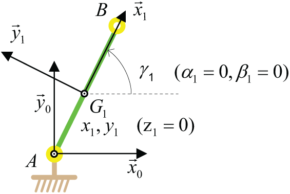
The authors selected the Tiernego and Bos³⁸ method for modelling multibody systems with bond graphs, because it allows a modular approach. This method enables a multibody system to be built as an assembly of bodies and joints and is based on the use of absolute coordinate systems (Figure 1) and Newton–Euler equations. The dynamic equations of a rigid body therefore depend on its mass/inertia properties and on geometric parameters for the body under consideration. The kinematic joints constrain the effort and flow vectors associated with the articulation points in the assembly of two bodies, so that the desired relative motion can be achieved. Consequently, the dynamic equations of the complete system consist of the dynamic equations of each body, in terms of its own parameters and the constraint equations of each joint.

Figure 1.

Parametrization of the free rigid body.

Modelling rigid bodies

Consider the architecture of a rigid body multibond graph model based on the literature.^1,6,42,43

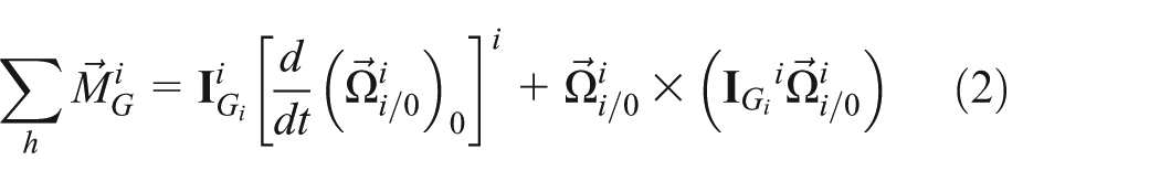
This bond graph architecture is based on the Newton–Euler equations (equations (1) and (2)). The inertia matrix $I_{G_{i}}$ , modelled with the multiport energy store element I in the upper part of Figure 2, is associated with gyroscopic terms which are modelled with a multiport gyrator element – also called Eulerian junction structure – about the centre of mass of body i expressed in its coordinate frame $EJ S_{G_{i}}$ . The mass matrix $m_{i}$ is modelled with a multiport energy store element I, shown in the lower part of Figure 2

\sum_{h} {\vec{F}}_{h \to j}^{0} + {\vec{P}}_{pes \to j}^{0} = m_{j} \frac{d}{dt} {({\vec{V}}_{G_{j} / 0}^{0})}_{0}

(1)

\sum_{h} {\vec{M}}_{G}^{i} = I_{G_{i}}^{i} {[\frac{d}{dt} {({\vec{Ω}}_{i / 0}^{i})}_{0}]}^{i} + {\vec{Ω}}_{i / 0}^{i} \times ({I_{G_{i}}}^{i} {\vec{Ω}}_{i / 0}^{i})

(2)

Figure 2.

Bond graph model of the rigid body.

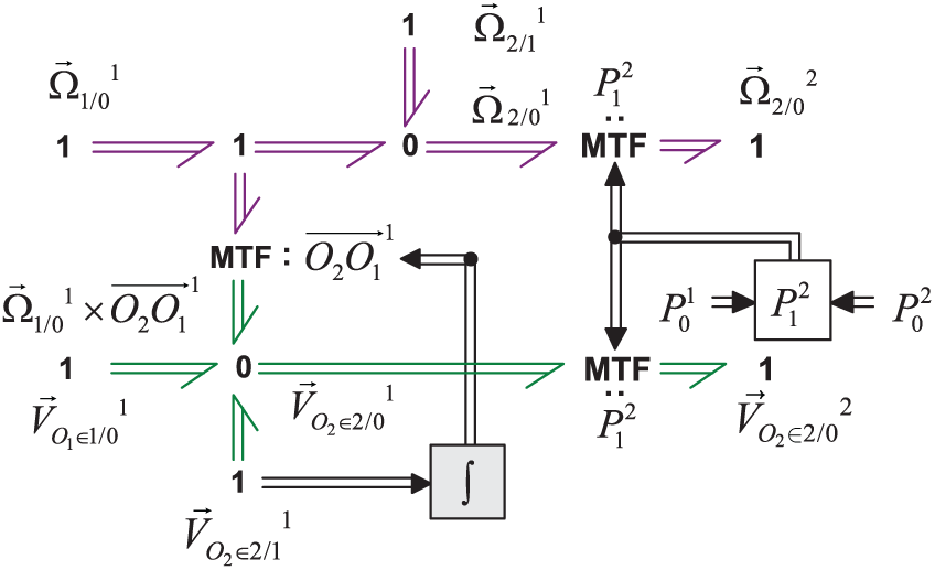
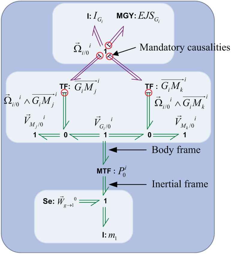
The upper part of the bond graph in Figure 2 represents the rotational dynamic part expressed in the body frame, while the lower part is for the translational dynamic part expressed in the inertial reference frame (or Galilean frame). Note that the power bonds corresponding to the rotational quantities are marked in purple, while the power bonds corresponding to the translational quantities are in green. 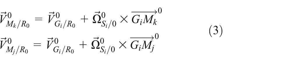The two 1-junction arrays correspond to the angular velocity vector of body j with regard to the inertial frame $\vec{Ω} (i / 0)^{i}$ and the translational velocity vector of body i’s centre of mass with regard to the inertial frame $\vec{V} (G_{i} / 0)^{0}$ , respectively.

The central part of Figure 2 describes the kinematic relations (equation (3)) between the velocities of the two points of the body i ( $\vec{V} (M_{j} / 0)^{i}$ and $\vec{V} (M_{k} / 0)^{0}$ ) and the velocity of the centre of mass $\vec{V} (G_{i} / 0)^{i}$ resulting from the formula of the rigid body

\begin{matrix} {\vec{V}}_{M_{k} / R_{0}}^{0} = {\vec{V}}_{G_{i} / R_{0}}^{0} + {\vec{Ω}}_{S_{i} / 0}^{0} \times {\vec{G_{i} M_{k}}}^{0} \\ {\vec{V}}_{M_{j} / R_{0}}^{0} = {\vec{V}}_{G_{i} / R_{0}}^{0} + {\vec{Ω}}_{S_{i} / 0}^{0} \times {\vec{G_{i} M_{j}}}^{0} \end{matrix}

(3)

As the translational dynamic is expressed in the inertial reference frame, a modulated transformer (MTF) element between ${\vec{V}}_{G_{i} / R_{0}}^{i}$ and ${\vec{V}}_{G_{i} / R_{0}}^{0}$ transforms the coordinates (equation (4)) between the body frame R_i and the inertial frame R₀

{\vec{V}}_{G_{i} / 0}^{0} = P_{0}^{i} \cdot {\vec{V}}_{G_{i} / 0}^{i}

(4)

In this article, XYZ Cardan angles have been employed for the sake of simplicity. The rotation matrix $P_{0}^{i}$ can be calculated from Cardan angles. The components of angular velocity for each body expressed in the body frame (the pseudo-velocities or rates of change of Cardan angles) are used to determine the body’s orientation and the corresponding coordinate transformation matrix. This classical process is used in the Cardan block detailed in Figure 3. It should be noted that the initial conditions for the integration of time derivatives must be consistent with regard to the kinematic constraints.

Figure 3.

Calculation of the Cardan angles and rotation matrix from the angular velocity.

It can be noted that the finite rotation transformation should be also defined with other coordinate systems since this transformation is a powerful conservative, for example, Euler angles with angles which are compatible with the mechanism concerning the singularities aspects, the Rodrigues–Hamilton parameters or the Cayley–Klein parameters. The implementation of the finite rotation transformation with the Rodrigues–Hamilton parameters is given by Marquis-Favre.⁴³

Modelling kinematic joints

The joint models express the constraints that are introduced when rigid bodies are connected. As with the bond graph model of the rigid body, the joint models have been built in a modular way, that is, their models do not change when the whole model of the system is assembled. The idea of this section is to allow bond graph practitioners to use a library of all the common existing kinematic joint models.

General kinematic joint model

The modelling of kinematic joints determines the rotational or translation degree of freedom (DOF) allowed by the joint.

Flow sources can be used to suppress the joint’s DOFs. However, in order to circumvent the causality constraints mentioned before, the joint models are presented with an additional L element which is either an R/C element or a modulated effort source (MSe) depending on the choice of simulation method (R/C element methods or the use of Lagrange multipliers).

For the unconstrained DOFs, the choice of modelling assumptions can dictate additional elements. If the joints are assumed to be perfect (i.e. without any dissipation or energy storage), there are no additional elements. However, if dissipation or compliance is assumed in the joints, R/C elements are added at the corresponding 1-junction. These R/C elements will be called as functional elements and should not be confused with the R/C elements used as parasitic elements for the purpose of simulation in section ‘The R/C parasitic element’.

The joint model is built from the following kinematic relationships

{\vec{Ω}}_{1 / 0}^{1} = {\vec{Ω}}_{1 / 2}^{1} + {\vec{Ω}}_{2 / 0}^{1}

(5)

where ${\vec{Ω}}_{1 / 0}^{1}$ is the absolute velocity of body 1 expressed in $R_{1}$ frame; ${\vec{Ω}}_{1 / 2}^{1}$ is the relative angular velocity of body 1 with regard to body 2 expressed in $R_{1}$ frame; ${\vec{Ω}}_{2 / 0}^{1}$ is the absolute velocity of body 2 expressed in $R_{1}$ frame; and

\begin{matrix} {\vec{V}}_{O_{2} \in 2 / 0}^{1} = {\vec{V}}_{O_{2} \in 2 / 1}^{1} + {\vec{V}}_{O_{2} \in 1 / 0}^{1} \\ = {\vec{V}}_{O_{2} \in 2 / 1}^{1} + ({\vec{V}}_{O_{1} \in 1 / 0}^{1} + {\vec{Ω}}_{1 / 0}^{1} \times {\vec{O_{1} O_{2}}}^{1}) \end{matrix}

(6)

which can be also written as

{\vec{V}}_{O_{2} / 0}^{1} = {\vec{V}}_{O_{2} \in 2 / 1}^{1} + ({\vec{V}}_{O_{1} / 0}^{1} + {\vec{Ω}}_{1 / 0}^{1} \times {\vec{O_{1} O_{2}}}^{1})

(7)

where ${\vec{V}}_{O_{2} / 0}^{1}$ is the absolute velocity of point O₂; ${\vec{V}}_{O_{1} / 0}^{1}$ is the absolute velocity of point O₁; ${\vec{V}}_{O_{2} \in 2 / 1}^{1}$ is the relative velocity of point O₂ with regard to the frame $R_{1}$ ; and ${\vec{Ω}}_{1 / 0}^{1} \times {\vec{O_{1} O_{2}}}^{1}$ is the velocity component due to the rotation of frame $R_{1}$ with regard to the inertial reference frame.

The general kinematic joint model is then detailed in Figure 4.

Figure 4.

General kinematic joint model.

In the general kinematic joint model, MTF elements modulated by coordinate transformation matrix are used to express the kinematic quantities in the frame associated with the body they are connected to.

Kinematic joint models

Based on the general kinematic joint model, models of common kinematic joints are given in Figures 5 –7.

Figure 5.

Kinematic joint models – part 1.

Figure 6.

Kinematic joint models – part 2.

Figure 7.

Kinematic joint models – part 3.

Methodology of modelling for simulation

General aspects

The first two steps of modelling a multibody system with bond graphs are choosing the dimension of the multibody model (2D or 3D) and choosing the dimension of the bonds (scalars or vectors).

In keeping with the philosophy of a modular approach, the authors propose a 3D model and vector bonds. Depending on the modelling objectives, the user can transform the model to one with scalar bonds in order to exploit it later (as described in Figure 8).

Figure 8.

Steps for the bond graph exploitation of MBS.

Hence, modelling with vector bonds is discussed first, and then with scalar bonds.

Modelling with vector bonds

The first step in carrying out a simulation of a bond graph is the assignment of causalities. Two causality constraints appear with vector bonds, as noted by Ersal et al.²⁴ and Behzadipour and Khajepour.⁴⁴

The first causality constraint (C1) is as follows:

C1: each component of a vector bond must have the same causality

Consequently, it is not possible to constrain the motion using Sf elements in only one or two dimensions without introducing some parasitic elements into the remaining unconstrained dimension(s).

The second causality constraint (C2) is as follows:

C2: the causality of transformers implied in the cross products and the causality of gyrators in the bond graph model of the rigid body are intrinsically fixed

The transformers implied in the cross products must have flow-in-flow-out causality;

The gyrators must have flow-in causality.

Indeed, contrary to scalar bond graphs, the ideal two-port elements cannot propagate causality in both directions when the moduli are not invertible. In the context studied here (i.e. multibody system modelling with bond graphs and the Tiernego and Bos approach), the cases in which moduli (matrices associated to the elements) are not invertible are present for two elements: the transformer (TF) between the rotational and translational domain and the gyrator (GY) since both elements implement cross products. Consequently, transformers and gyrators have the mandatory fixed causality assignment specified above. The transformers and gyrators with the acceptable causal forms mentioned are given in Figure 9.

Figure 9.

Causalities imposed with (modulated) TF and GY elements.

The causalities imposed on the transformers lead to some specific results when multibody systems with kinematic loops are considered. Figure 10 presents the bond graph model of a rigid body with vector bond and the imposed causalities. Consequently, in the bond graph of a rigid body, attaching flow sources (Sf) to more than one hinge point or the centre of mass at the same time is not possible and leads to causality conflicts. This situation typically occurs when the multibody system is composed of kinematic loops. Ersal et al.²⁴ give the example of an oscillating bar which, with its two joints, is a CKC system with one body. This case will appear in the slider crank model presented in this article.

Figure 10.

Bond graph model of rigid body with vector bonds and the imposed causalities.

Modelling with scalar bonds

Bond graph models with scalar bonds do not have the same causality constraints as vector multibonds. However, in order to obtain the bond graph model with scalar bonds in a systematic way from the vector bond model, the same causality constraints (C1 and C2) on the gyrators and the transformers used for cross products are kept. Consequently, following the method chosen for the simulation of the bond graph model (presented in section ‘Review of the simulation methods’), the scalar equivalent transformers representing coordinate transformation (here called coordinate transformation subsystems) should be adapted to respect the causality imposed by the rest of the bond graph. This is true for both the rigid bodies and the joints. The causality of these transformers depends on the elements used to constrain the motion.

These coordinate transformation subsystems can have two different structures: the structure with flow-in-flow-out causality and the structure with effort-in-effort-out causality. The causalities of these coordinate transformation subsystems are imposed by the position of the 0-junctions or 1-junctions with regard to the scalar MTFs. The coordinate transformation subsystem with flow-in-flow-out causality is built with the 1-junctions at its input in order to propagate causality to the rest of the elements. Following the same logic, the coordinate transformation subsystem with effort-in-effort-out causality is built with the 0-junctions at the input.

Figure 11 presents the two possible structures of the coordinate transformation subsystem and the cross product model for the bond graph model of the rigid body. The use of these coordinate transformation subsystems in the joints is illustrated in section ‘Case studies’ of this article (see Figure 19). For the sake of clarity, the modulation signals for the MTFs are not displayed. Figures 12 and 13 present, respectively, the rotational dynamic model and translational dynamic model in scalar bond graphs. To the authors’ knowledge, these models have been presented for the first time in this form in the work of Ersal et al.^27,45

Figure 11.

Bond graph model of rigid body with scalar bonds.

Figure 12.

Rotational dynamics.

Figure 13.

Translational dynamics.

The procedure for transforming a multibody model with vector bonds into one with scalar bonds is as follows:

Identify the causality of the transformers linked to coordinate transformation (in bodies and joints).

Replace each of these transformers with the appropriate transformer subsystems and assign the same causality as that seen on the vectorial MTF in the model with vector bonds:

(a) If the vectorial MTF is flow-in-flow-out causality, then use the coordinate transformation subsystem with flow-in-flow out causality (with 1-junctions at the input and 0-junctions at the output).

(b) If the vectorial MTF is effort-in-effort-out causality, then use the coordinate transformation subsystem with effort-in-effort-out causality (with 0-junctions at the input and 1-junctions at the output).

Differential-algebraic equation formulation

In this article, absolute coordinates are selected in order to keep a modular approach. Consequently, due to the kinematic constraints, derivative causality appears on the inertial elements and leads to differential-algebraic equations (DAEs). It is important to note that both OC and CKC systems therefore lead to a DAE formulation. One of the priorities of the simulation methods proposed in this article will therefore be to handle DAEs.

Review of the simulation methods

The methods presented in this section come from the references given in section ‘Brief review’. The value of this study is in giving practical guidelines to modellers, so that they can implement the adapted method in 20-sim software.

Minimal coordinate method

Description

The minimal coordinate method is based on formulating the dynamics using minimal set of joint coordinates (as generalised coordinates) to describe the DOFs of the mechanism.

Tiernego and Bos method leads to a model with a mixed differential-integral causalities on its inertial elements. The number of variables of inertial elements with derivative causalities depends on the variables of the inertial elements with integral causalities. The principle of the method is to transform the dependent inertia storage element (using transformers) and to combine them with the independent elements. This idea was first described in the context of bond graphs by Karnopp.³

Allen⁴⁶ uses this transformation on multibody systems where the dynamics are described with Lagrange equations and generalised coordinates. Breedveld and Hogan⁷ utilise it on a rigid body dynamic model corresponding to Newton–Euler equations with absolute coordinates. From a bond graph point of view, the minimal coordinate method consists of a two-level transformation through transformer elements as detailed in Figure 14. One level of transformers converts the velocities associated with inertial elements in absolute coordinates to the generalised velocities chosen as the joint’s coordinates (also called relative coordinates). The second level of transformers converts the generalised velocities to the independent generalised velocity vector.

Figure 14.

Equivalent mechanism bond graph model in relative coordinates.

As mentioned in section ‘Modelling rigid bodies’, the dynamics of a mechanism are represented by two elements. The rotational dynamics of a mechanism are described by I-elements, characterised by the inertia tensor I of the body and the corresponding gyrator MGY. The translational dynamics are also described by an I-element, characterised by the mass tensor m_i.

For a system of n DOFs, there are n independent velocities grouped in vector ${\overset{\cdot}{q}}_{i}$ . The generalised velocity vector $\overset{\cdot}{q}$ defined for a mechanism can be partitioned into independent and dependent generalised velocities as follows

\overset{\cdot}{q} = [\begin{matrix} {\overset{\cdot}{q}}_{i} \\ {\overset{\cdot}{q}}_{d} \end{matrix}]

(8)

The dependent generalised velocities can be written as a function of the independent generalised velocities

{\overset{\cdot}{q}}_{d} = T {\overset{\cdot}{q}}_{i}

(9)

where $T$ is a displacement-dependent velocity transformation between dependent and independent generalised velocities.

From equations (8) and (9), the generalised velocities can be written as a function of the independent generalised coordinates

\overset{\cdot}{q} = M_{β} {\overset{\cdot}{q}}_{i}

(10)

with $M_{β} = [\begin{matrix} 1 \\ T \end{matrix}]$ . This notation is inspired by Allen.⁴⁶

The inertial velocities of each body can be written as a function of the generalised velocities

V_{i} = T_{i} \overset{\cdot}{q}

(11)

where $T_{i} = T_{Ω_{i}} or T_{V_{i}}$ are the displacement-dependent velocity transformations between inertial and generalised velocities.

Allen⁴⁶ shows that the transformation of multiport inertia elements over an MTF transformation leads to a virtual inertia Ĩ and a modulated gyristor element MGR. The ‘virtual’ denomination comes from the fact that the terms of this inertia are not constant. The modulated gyristor MGR comes from the MTF with a variable modulus. In the study of Breedveld and Hogan,⁷ Breedveld formulated the displacement of I-elements and the gyrator GY element over a transformation from the inertial velocities to the generalised velocities. This leads to the following equations

{\tilde{I}}_{1} = \sum_{i} T_{Ω_{i}}^{T} \cdot I_{G_{i}} \cdot T_{Ω_{i}} + \sum_{i} T_{V_{i}}^{T} \cdot m_{i} \cdot T_{V_{i}}

(12)

MG R_{1} = \sum_{i} T_{Ω_{i}}^{T} \cdot I_{G_{i}} {\overset{\cdot}{T}}_{Ω_{i}} + \sum_{i} T_{V_{i}}^{T} \cdot m_{i} \cdot {\overset{\cdot}{T}}_{V_{i}}

(13)

EJ S_{1} = \sum_{i} T_{Ω_{i}}^{T} \cdot EJ S_{G_{i}} \cdot T_{Ω_{i}}

(14)

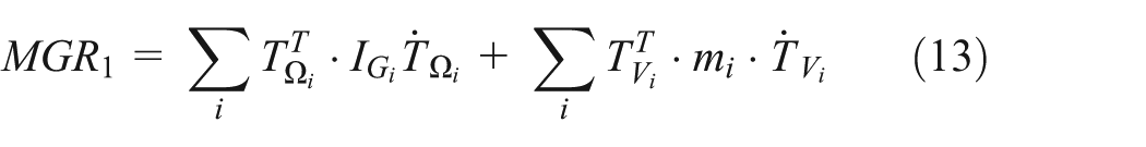
The second transformation leads to the virtual inertia Ĩ₂, gyristor MGR₂ and junction structure EJS₂ associated with the independent generalised velocities. These are both modulated by the independent generalised parameters q_i

\begin{matrix} {\tilde{I}}_{2} = \sum_{i} M_{β}^{T} \cdot T_{Ω_{i}}^{T} \cdot I_{G_{i}} \cdot T_{Ω_{i}} \cdot M_{β} + \sum_{i} M_{β}^{T} \\ \cdot T_{V_{i}}^{T} \cdot m_{i} \cdot T_{V_{i}} \cdot M_{β} \end{matrix}

(15)

\begin{matrix} MG R_{2} = \sum_{i} M_{β}^{T} \cdot T_{Ω_{i}}^{T} \cdot I_{G_{i}} \cdot (T_{Ω_{i}} \cdot {\overset{\cdot}{M}}_{β} + {\overset{\cdot}{T}}_{Ω_{i}} \cdot M_{β}) \\ + \sum_{i} M_{β}^{T} \cdot T_{V_{i}}^{T} \cdot m_{i} \cdot (T_{V_{i}} \cdot {\overset{\cdot}{M}}_{β} + {\overset{\cdot}{T}}_{V_{i}} \cdot M_{β}) \end{matrix}

(16)

EJ S_{2} = \sum_{i} M_{β}^{T} \cdot T_{Ω_{i}}^{T} \cdot EJ S_{G_{i}} \cdot T_{Ω_{i}} \cdot M_{β}

(17)

The bond graph of the two-level transformation is given in Figure 15.

Figure 15.

Displacement of I and GY elements through two-level transformers.

This method requires three steps of symbolic manipulations. The first one is the determination of the $T_{i}$ and $M_{β}$ matrices from the kinematic relations. The second is the derivation of these matrices, which is required for the construction of the MGR elements. The third is the multiplication of non-linear matrices for the final computation of the added elements. Allen⁴⁶ conducts manual symbolic manipulation so as to determine the velocity relations from the displacement equations obtained by geometric analysis. Bos⁶ has improved this method using the bond graph to derive the velocity’s transformation. Felez et al.⁴⁷ and Borutzky¹ later presented a similar method to systematically deduce the kinematic relations from a modified bond graph model by the addition of controlled flow sources.

The technique of transforming storage elements from dependent to independent has been applied on industrial mechanisms: a forming machine,^46,48 a web cutting machine,⁴⁹ a pneumatic welding robot⁵⁰ and manipulator robots.⁵¹ More recently, bond graph examples have been published: a planar pendulum in the work of Breedveld⁵² and a simple slider crank modelled from Lagrange equations using Karnopp procedure in the work of Borutzky.¹ In this article, it is applied on a slider crank modelled with the modular Bos and Tiernego method and can be easily used for more complex systems. As Borutzky¹ points out, this method essentially applies the well-known joint coordinate formulation of Nikravesh and Gim⁵³ to the bond graph modelling of multibody systems.

Advantages

All derivative causalities are removed, and only integral causality remains on the inertia associated with the independent generalised velocity vector. The virtual inertia will always be in integral causality because it is grouped to an inertia element in integral causality during the transformation. Consequently, the number of equations is reduced and an ordinary differential equation (ODE) formulation is achieved, which is much more compact than a DAE system. The ODE model can be solved with a fixed step solver such as fourth-order Runge–Kutta method.

Drawbacks

The technique can be very demanding in terms of computer memory, and requires consistent mathematical simplifications by an expert user.

The modularity (i.e. the property whereby the mechanism can be assembled as a set of subsystems according to its structure) disappears. Hence, simulation of a mechanism’s subsystems can no longer be conducted individually to check the whole model one piece at a time.

Zero-order causal path opening method

Description

Once causality is applied, different types of causal paths between elements can be identified. A closed causal path without any integration operations is called a zero-order causal path (ZCP).^22,54–57 Bond graphs with ZCPs generate mathematical models with DAEs. There is a direct link between the nature of the ZCPs in the bond graphs and the index of the DAEs. The definitions of ZCPs are given by Felez et al.²² as follows:

Class 1 ZCPs: The causal path is set between storage ports with integral causality and storage ports with differential causality. The associated topological loops are flat.

Class 2 ZCPs: The causal path is set between elements whose constitutive relations are algebraic (resistors are the most typical case). The topological loops are flat.

Class 3 ZCPs: A causal cycle whose topological loops are open. The causal path starts and ends in the same port of an element.

Class 4 ZCPs: Causal cycles whose topological loops are closed.

Only Class 4 ZCPs lead to DAEs with an index of 2. When the DAE’s index is inferior to 2, a backward differentiation formula (BDF) solver (such as the one in 20-sim) can handle these equations. In some cases (scalar bonds or vector bonds with no kinematic loops), the simulation can thus be conducted without additional specific elements.

Advantages

First, this method enables simulations to be conducted directly from the model without requiring the addition of elements (R/C elements or controlled effort sources) at the correction location. The initial physical model is therefore not changed. Second, this method is faster than the two following methods (R/C elements and controlled effort sources), as demonstrated in section ‘Case studies’.

Drawbacks

When multibody systems have kinematic loops, the bond graph may contain class-4 ZCPs which lead to a DAE formulation with an index superior to 1. When this happens, the BDF solver often encounters difficulties in the numerical computation of the model. The ZCP opening method consists of opening the class-4 ZCP using ‘break variables’. This technique can be used at an equation level or at a graphical level. The classical technique uses modulated sources (MSe) at 1-junctions of the class-4 ZCPs to open them. Without a systematic approach to the detection of the class-4 ZCPs, this method may be difficult to use when dealing with a case that involves complex multibody systems. Hence, the authors have not used this method here.

R/C parasitic element

Description

The R/C parasitic element method first appears as the ‘Stiff-compliance’ approach in the study of Karnopp and Margolis.⁵⁸ In the literature, other terminologies can be found: singular perturbation,⁵⁹ parasitic elements,^23,60 virtual springs⁶¹ and coupling or pads^21,62

This method is based on the introduction of parasitic elements: compliances and resistances in the bond graph models of the joints. When used with multibody systems, this method has two objectives: (1) eliminating the kinematic constraints and (2) eliminating the derivative causality (which yields algebraic loops) so that an explicit solver may be used.

As mentioned in section ‘Modelling with vector bonds’, vector bond graphs impose some supplementary causality constraints (C1 and C2). These constraints can be enforced using flow sources (Sf), but they may lead to causal conflicts because of their flow-out causality. Enforcing the constraints with parasitic elements (R/C elements) can circumvent these conflicts since they can take effort-out causality. First, they allow the preservation of the causality assignments for all bonds of a multibond (C1 respected). Second, they allow the suppression of causality conflicts which may appear due to the causality of the transformers implied in the cross product and gyrators (C2 respected).

Advantages

With the R/C parasitic element method, all derivative causalities are removed. This leads to an explicit ODE model, which can be solved with a fixed step solver such as fourth-order Runge–Kutta method.

Unlike the Lagrange multiplier method, the consistency between the initial conditions for CKC system is not mandatory. In the work of Rideout,²³ the parasitic element method is even used to determine initial conditions. In addition, over-constrained (also called hyperstatic) systems can be simulated without any difficulties, as demonstrated in section ‘Case studies’. Karnopp and Rosenberg⁵ state that

The idea of using artificial C- and R-elements to enforce constraints and thus to avoid derivative causality or differential-algebraic equations may appear to be a ‘brute-force’ approach. This may be true, but first, a brute-force approach that is effective should not be discounted and, second, it has been argued that this approach is in many cases superior to the alternatives.

Drawbacks

This method introduces new elements (R/C elements) to the initial bond graph, whose parameters and initial conditions (in the case of C-elements) need to be specified. The values of the compliant elements must reflect the compliances which exist in all mechanical joints. The stiffness that is used should be high enough so as to approximate the constraints and not change the dynamics of the system. However, high stiffness can introduce high-frequency dynamics. This forces the solver to take very small integration steps to meet the tolerance criteria and, consequently, the simulation is slowed. This method therefore leads to a compromise between the accuracy of the results and the simulation time: the stiffer the system, the more numerical errors are reduced but the higher the simulation time.

Implementation

Even theoretically where explicit solvers can be used, the authors recommend the use of the implicit modified backward differentiation formula (MBDF) solver for three reasons. The first is because the MBDF solver is faster than classic explicit solver when a stiff ODE is concerned. The second is because, as an implicit method, the stability is guaranteed. The third is that controlled effort sources necessitate the use of the MBDF solver. Using the MBDF solver with R/C elements also allows comparison between the use of R/C elements and controlled effort sources. In this article, all simulations have been conducted with MBDF solvers.

Lagrange multiplier method

Description

In the Lagrange multiplier method, the constraint forces are modelled by controlled effort sources (MSe) rather than by parasitic elements. This method originates from Bos⁶ and Felez et al.⁴⁰ and has been implemented in 20-sim by Borutzky and Van Dijk.^1,41,63 The same concept is also implemented by Ersal et al.²⁴ with pseudo flow source (PSf) elements.

This method is similar to the parasitic elements in which the causality conflict is suppressed by removing the flow sources (Sf) and enforcing the constraint by other elements which do not have flow causality (here the controlled effort sources MSe)

The controlled effort sources (MSe) are computed such that the difference between velocities for the constraints is zero. The principle is to apply an effort equivalent to the one that the system would impose on a flow source. It would have a practical operation as a flow source but with effort-out causality instead of a flow-out causality.

The constitutive laws of the controlled effort sources are as follows:

The usual constitutive law for an effort source;

The constraint: effort = e such that flow(e) = f.

Figure 16 illustrates the implementation of this constraint. The effort e(t) applied iteratively to the system is determined so that the difference ε(t) between the flow measurement f(t) and its set point f_c(t) tends to zero. This implementation uses the constraint() function in 20-sim. At every simulation step, this function induces an iterative procedure to find the force that keeps the velocity offset at zero within a given error margin. This iterative procedure is only supported by the MBDF in 20-sim software.

Figure 16.

Implementation of the controlled effort source.

The effort-out causality of the controlled effort sources ensures that all the inertial elements (I elements) receive integral causality. The dependent states are therefore not visible as derivative causality. However, the controlled effort source establishes within itself algebraic dependencies and thus indicates an implicit form of equations. As stated by Borutzky,¹ the DAE system has an index of 2 due to the fact that the constraint forces do not appear in the algebraic constraints but is in a semi-explicit form which can be solved by the MBDF solver.

Advantages

Contrary to the parasitic element method, the modulated sources (MSe) do not need additional tuning because no additional parameters are added to the system. In other words, the order of the system is not modified because no new states (with their associated parameters and initial conditions) are introduced. The absence of supplementary parameters creates a bond graph that describes the system ideally, within the limit of the numerical tolerance on the constraints equations.

Although some iterations are required during the simulation to satisfy the constraint equations at each time step, the computational load is comparable or better than the parasitic element method, where the differential equations are truly explicit but very stiff.

Drawbacks

The bond graph obtained with this approach leads to implicit differential equations. Explicit integration algorithms therefore cannot be used, and the constraints can only be met within some numerical tolerances during the simulation. Consequently, the implementation of this method requires care.

Implementation

The Lagrange multiplier method is more challenging to implement than R/C elements, because the kinematic constraints imposed by the joints may produce computational conflicts. This issue occurs on CKCs with over-constrained multibody systems. Due to the topology of the system, more than one joint could impose the same constraint on the system, in which case the simulation will no longer be possible. The number of the controlled effort sources must not exceed the DOFs that need to be eliminated.

In order to solve this problem, the redundant constraints must be removed. For the slider crank example in the last section of this article, a practical detection method will be applied to determine the redundant constraints.

The initial conditions of the system should be consistent with constraints. If a controlled effort source is attached to a 1-junction to keep the velocity at zero, and a non-zero initial velocity is imposed on an I-element connected to the same 1-junction, then a simulation cannot be conducted. Note at this point that 20-sim does not offer an automatic correction of inconsistent initial conditions, but the user can always code the calculation of consistent initial conditions.

Case studies

The systems chosen here are intentionally kept simple, in order to demonstrate the methods for simulating bond graph models of multibody systems. Two classical systems are chosen: (1) the planar pendulum as an example of an OC system and (2) the slider crank as an example of a CKC system. The physical models parameterized with absolute coordinate systems are given in Figures 17 and 22. The values of model parameters are given in Appendix 1. For ease of representation, the physical models are given with a planar representation. However, the bond graph models have been realised on 3D physical models. This will impact the modelling of the crankshaft, which only contains redundant constraints when modelled in 3D.

Figure 17.

Physical model of a planar pendulum.

Planar pendulum

Mechanical scheme

The physical model of a planar pendulum is shown in Figure 17.

Modelling with vector bonds

The models of the planar pendulum with the vector bonds are presented in Figure 18. Note that, when the Tiernego and Bos method is applied (ZCP method), inertial elements with differential causalities are present. When R/C or controlled effort source methods are used, integral causalities are conserved in the inertial elements.

Figure 18.

Bond graph models with vector bonds of a planar pendulum.

Modelling with scalar bonds

The models of the planar pendulum with scalar bonds are presented in Figure 19.

Figure 19.

Bong graph models with scalar bonds of a planar pendulum.

Simulation results

For the ZCP method, the equations are DAEs because of the inertial elements with differential causalities. However, since the ZCPs are class 2 or 3 (not 4), 20-sim’s BDF solver can handle the DAE. For the R/C method, the inertial elements with integral causalities lead to explicit differential equations, which could be easily integrated using explicit algorithms such as fourth-order Runge–Kutta method. In order to compare the three methods (ZCP, R/C and MSe), the BDF solver in 20-sim is used. For the Lagrange multiplier method, the dependencies are not visible in the form of derivative causality, but the equations still take an implicit form. Consequently, as previously discussed, explicit integration algorithms cannot be used.

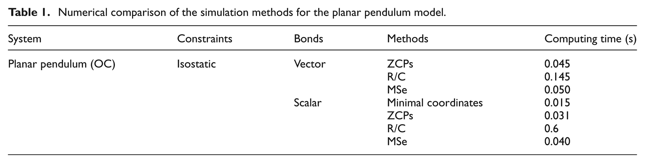
From the results obtained (Table 1), similar conclusions to Borutzky⁴¹ can be made. The ZCP method is the fastest of the three methods. The computational time of the Lagrange multiplier method is still comparable to the ZCP method but needs the addition of elements: the control effort sources. It can also be seen that there is a slight difference in computational time between the models with scalar bonds and vector bonds. The models with vector bonds take a little longer to simulate than the ones with scalar bonds.

Table 1.

Numerical comparison of the simulation methods for the planar pendulum model.

System	Constraints	Bonds	Methods	Computing time (s)
Planar pendulum (OC)	Isostatic	Vector	ZCPs	0.045
			R/C	0.145
			MSe	0.050
		Scalar	Minimal coordinates	0.015
			ZCPs	0.031
			R/C	0.6
			MSe	0.040

In order to test the accuracy of the solution, these methods are compared to a bond graph model with minimal coordinates. This is the simplest possible model, presented in the study of Breedveld⁵² and recalled in Figure 20. From the results obtained (Figure 21), it can be seen that the ZCP method is almost identical to the bond graph with minimal coordinates. The R/C method yields a short ‘peak’, which is due to the excitation of the modes introduced by these elements.

Figure 20.

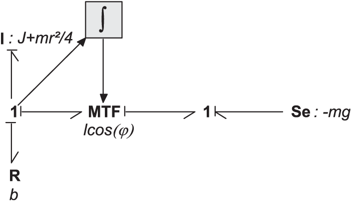
Planar pendulum with minimal coordinates.

Figure 21.

Difference in the different methods (ZCP, Lagrange and singular perturbation with regard to the model with minimal coordinates) on the angular velocity.

Slider crank

Mechanical scheme

Classically, the slider crank is composed of three bodies: the crank, the rod, and the piston, and four joints. Depending on the choice of the joints on CKC system, a hyperstatic system (also called an over-constrained system) can appear. That is the case when the slider crank comprises three revolute joints and one prismatic joint (Figure 22). In this case, the system is over-constrained because the number of constraints is higher than the relative DOF after connection (shown in Table 2). The last line of the table corresponds to the remaining DOFs after having closed the kinematic loop.

Figure 22.

Physical model of a hyperstatic slider crank.

Table 2.

Analysis of the hyperstatic slider crank model.

Stage	Joint concerned	Relative DOF	Joint type	No. of constraints	Relative DOF after connection
1	Fixed frame and crank	6	Revolute joint	5	1
2	Crank and rod	6	Revolute joint	5	1
3	Rod and piston	6	Revolute joint	5	1
4	Piston and fixed frame	1 + 1 + 1 = 3	Prismatic joint	5	−2

This mechanical model can be modified into an isostatic one (Figure 23). The method is based on the reduction of DOFs from the reduction of constraints, as shown in Table 3.

Figure 23.

Physical model of an isostatic slider crank.

Table 3.

Analysis of the isostatic slider crank model.

Stage	Joint concerned	Relative DOF	Joint type	No. of constraints	Relative DOF after connection
1	Fixed frame and crank	6	Revolute joint	5	1
2	Crank and rod	6	Rotational joint	4	2
3	Rod and piston	6	Spherical joint	3	3
4	Piston and fixed frame	1 + 2 + 3 = 6	Prismatic joint	5	1

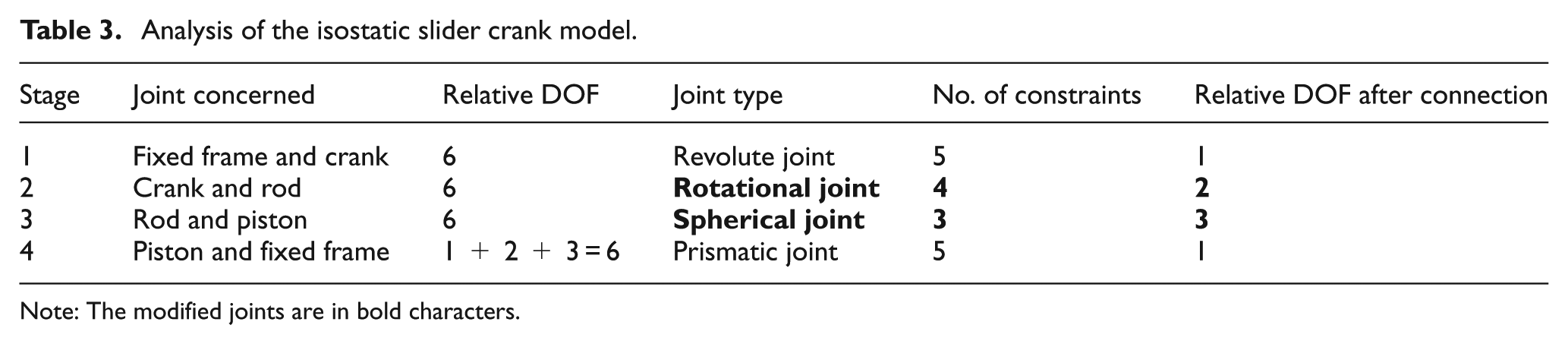
Note: The modified joints are in bold characters.

The redundant coordinates can be determined automatically using a structural multibody tool such as MapleSIM.⁶⁴ The process of identifying and removing constraints is done numerically. MapleSIM achieves this by obtaining the Jacobian and residual of all the constraints, and then performing numerical projections to determine which rows/constraints have the most effect on the condition of the matrix.

A summary of the two models studied is presented in Table 4.

Table 4.

Main characteristics of the two slider crank models.

	Hyperstatic slider crank model	Isostatic slider crank model
No. of coordinates	18 (3 bodies)	18 (3 bodies)
No. of constraints	203 revolute joints (5 DOFs)+1 prismatic joint (5 DOFs)	171 revolute joint (5 DOFs)+1 rotational joint (4 DOFs)+1 spherical joint (3 DOFs)+1 prismatic joint (5 DOFs)
Kinematic mobility	1	1
Over-constraints	3	0

The different structure of the mechanical model (hyperstatic or isostatic) plays an important role in the simulation as shown in the next section.

Hyperstatic model

Modelling with vector bonds

The bond graph model of the hyperstatic slider crank with vector bonds and R/C element method is presented in Figure 24. The R/C method relaxes the kinematic joint constraints. The dynamic equations are therefore transformed into an ODE form with no geometric constraints to deal with. Consequently, this method easily permits the simulation of hyperstatic CKC systems. In fact, the added springs have a very strong stiffness to keep a physical behaviour close to a rigid joint but, from a computational point of view, the hyperstatic nature of the model has disappeared thanks to the addition of the R/C elements.

Figure 24.

Bond graph model with vector bonds and R/C element method of the hyperstatic slider crank.

When over-constraints are present, the Lagrange multipliers create more difficulties than the use of R/C element methods. In this case (CKC system), more than one joint could impose the same constraint on the system. In order to solve the model with Lagrange multipliers, the redundant constraints must be eliminated. For that purpose, the model has to be changed to an isostatic one by joint altercation.

Modelling with scalar bonds

The model with scalar bonds and R/C elements is built with the procedure given in section ‘Modelling with scalar bonds’.

Isostatic model

Modelling with vector bonds

When the definition of joints is modified by removing the redundant constraints, the simulation of the isostatic model can be conducted with both the R/C element and Lagrange multiplier methods. The bond graph model of the isostatic slider crank with vector bonds and MSe elements is presented in Figure 25.

Figure 25.

Bond graph model with vector bonds and MSe elements of the isostatic slider crank.

Modelling with scalar bonds

The models with scalar bonds are built in a similar way for both the R/C method and the Lagrange multiplier method. The bond graph model of the isostatic slider crank with scalar bonds and MSe elements is presented in Figure 26.

Figure 26.

Bond graph model with scalar bonds and MSe elements of slider crank.

Minimal coordinate model

In order to test the accuracy of the solution, these methods are again compared to a bond graph model with a minimal coordinate formulation. The method is presented in section ‘Minimal coordinate method’ and results from the isostatic model previously described. The kinematic scheme of the slider crank with geometric parameters is detailed in Figure 27. Note that only three parameters (x_i, y_i, γ_i) for the absolute coordinates are shown in this planar scheme but, in the bond graph models, six parameters (x_i, y_i, z_i, α_i, β_i, γ_i) are considered for the absolute coordinates. The bond graph model is presented in Figure 28. All the dependent storage elements with derivative causality have been transformed by transferring the inertia of those elements to the independent storage element with integral causality (the angle of the crank $\overset{\cdot}{γ}$ ), using a virtual inertia and gyristor. The transformation matrices (from the inertial velocities to the generalised velocities, and the generalised velocities to the independent coordinate $\overset{\cdot}{γ}$ ) are given in Appendix 2.

Figure 27.

Kinematic scheme of the slidercrank.

Figure 28.

Slider crank model with minimal coordinates.

Simulation results

A simulation of the dynamics of these models has been conducted. Identical results to Rideout⁶⁵ have been obtained (Figures 29 and 30).

Figure 29.

Evolution of the centre of gravities in the inertial frame of the different bodies.

Figure 30.

Evolution of angles.

A comparison of results in terms of computing time of the simulation is presented in Table 5. The simulation of hyperstatic kinematic closed systems (such as the slider crank with three revolute joints) is possible with R/C elements as we have previously mentioned, and the simulation time of the hyperstatic system is comparable to the isostatic system. Both the R/C method and the Lagrange multiplier method have comparable computation times. Their computational loads are bigger than that of the minimal coordinates, but remain within acceptable limits. Finally, as in the planar pendulum, models with vector bonds always take a little longer to simulate than the ones with scalar bonds.

Table 5.

Numerical comparison of the simulation methods for the slider crank models.

System	Constraints	Bonds	Methods	Computingtime (s)
Slider crank(CKC)	Hyperstatic	Vector	R/C	0.5
	Hyperstatic	Scalar	R/C	0.45
	Isostatic	Vector	ZCPs	Hard to conduct
			R/C	0.51
			MSe	0.330
		Scalar	Minimalcoordinates	0.19
			ZCPs	Hard toconduct
			R/C	0.4
			MSe	0.300

For the ZCP method with both scalar and vector bonds, CKC systems induce several ZCPs of class 1 and 4. The class-1 ZCPs are associated with dependences between energy storage elements, whereas the class-4 ZCPs are associated with causal cycles along the junction structures. The DAE index will typically be greater than 1. Consequently, the model with ZCPs does not permit direct simulation with the MBDF solver. In order to enable simulation, a specific causality assignment or break variables should be used to reduce the DAE index. There is no automatic method for locating ZCPs on large bond graphs within platforms such as 20-sim at the time of writing. However, an automatic ZCP-location method would not significantly improve computation time and accuracy.

Figure 31 shows that the R/C method and the Lagrange multiplier method perform comparably to the minimal coordinate method, with errors of less than 4e-3 m/s. The errors are dependent of some parameters: the value of the R/C method or the value of the integration error accepted for the solver. The proposed values of R/C elements (parasitic stiffness = 10⁻⁷ N/m and parasitic damping = 200 N·s/m) are therefore considered satisfactory for this application.

Figure 31.

Difference between the different methods (Lagrange multipliers and R/C methods) and the model with minimal coordinates on the piston velocity.

Conclusion

This article presents three methods for simulating bond graph models of multibody systems: ZCP, R/C elements and Lagrange multipliers. For each method, the authors suggest implementing both conditions and practical rules for application. Additional considerations include the nature of the chain of multibody systems, the nature of the system towards its joint constraints, and the nature of the bonds.

A method for transforming vector bond graphs to scalar bond graphs is also provided. Future work will automate this.

Numerical comparisons complement the results given by Van Dijk and Breedveld⁴¹ and Felez et al.²² There is no best unique solution for conducting bond graph simulations of multibody systems: all of these methods are correct, and the best will depend on the application. The authors suggest the following guidelines:

The R/C method is perhaps the most convenient. It permits the simulation of both iso- and over-constrained multibody systems with kinematic closed loops. It is tolerant of small inconsistencies in the initial conditions and allows the use of a classical explicit solver. The computational time and accuracy are comparable to the other methods.

Lagrange multipliers must be implemented with care in the case of the over-constrained multibody systems, but give an ideal description of the system within the limit of the numerical tolerance on the constraint equations.

The ZCP method is easy and quick to implement on simple multibody systems. When applying it to large systems, a systematic way of detecting the class-4 ZCPs would be advantageous.

Footnotes

Appendix 1

Appendix 2

Handling Editor: Xiaoting Rui

Declaration of conflicting interests

The author(s) declared no potential conflicts of interest with respect to the research, authorship and/or publication of this article.

Funding

The author(s) received no financial support for the research, authorship and/or publication of this article.

ORCID iD

Benjamin Boudon

References

Borutzky

. Bond graph methodology – development and analysis of multidisciplinary dynamic system models. London: Springer, 2010.

Borutzky

. Bond graph modelling of engineering systems – theory, applications and software support. London: Springer, 2011.

Karnopp

. Power-conserving transformations: physical interpretations and applications using bond graphs. J Frankl Inst 1969; 288: 175–201.

Rosenberg

. Multiport models in mechanics. J Dyn Syst Meas Control 1972; 94: 206–212.

Karnopp

Rosenberg

. Systems dynamics: modeling, simulation, and control of mechatronics systems. 5th ed. Hoboken, NJ: John Wiley & Sons, 2012.

Bos

. Multibody systems in terms of multibond graphs with application to a motorcycle multibody system. Enschede: University of Twente, 1986.

Breedveld

Hogan

. Multibond graph representation of Lagrangian mechanics: the elimination of the Euler junction structure. In: Proceedings of mathmod’94 – International Association for Mathematics and Computers in Simulation (IMACS) symposium on mathematical modelling, Vienna, Austria, 2–4 February 1994.

Marquis-Favre

Scavarda

. A representation for planar point contact joints in the multibody mechanical bond graph library. Proc IMechE, Part I: J Systems and Control Engineering 1998; 212: 305–313.

Bera

Bhattacharya

Samantaray

. Evaluation of antilock braking system with an integrated model of full vehicle system dynamics. Simul Model Pract Th 2011; 19: 2131–2150.

10.

Nakhaeinejad

Bryant

. Dynamic modeling of rolling element bearings with surface contact defects using bond graphs. J Tribol 2011; 133: 011102.

11.

Damić

. Modelling flexible body systems: a bond graph component model approach. Math Comput Model Dyn Syst 2006; 12: 175–187.

12.

Cohodar

Borutzky

Damic

. Comparison of different formulations of 2D beam elements based on Bond Graph technique. Simul Model Pract Th 2009; 17: 107–124.

13.

Pacejka

. Modeling complex vehicles using bond graphs. J Frankl Inst 1985; 319: 67–81.

14.

Pacejka

. Development and validation of a bond graph handling model of an automobile. J Frankl Inst 1991; 328: 941–957.

15.

Hrovat

Tobler

. Bond graph modeling and computer simulation of automative torque converters. J Frankl Inst 1985; 319: 93–114.

16.

Hrovat

Tobler

. Bond graph modeling of automative power trains. J Frankl Inst 1991; 328: 623–662.

17.

Pathak

Mukherjee

Dasgupta

. Impedance control of space robots using passive degrees freedom in controller domain. Trans ASME 2005; 127: 564–578.

18.

Vaz

. Bond graph model of extensor mechanism of finger based on hook-string mechanism. Mech Mach Theory 2015; 91: 187–208.

19.

Dauphin-Tanguy

. Les bonds graphs: Paris: Hermès Sciences, 2000.

20.

Das

. Mechatronic modeling and simulation using bond graphs. Boca Raton, FL: CRC Press, 2009.

21.

Merzouki

Samantaray

Pathak

et al . Intelligent mechatronic systems – modeling, control and diagnostic. New York: Springer, 2013.

22.

Felez

Romero

Maroto

et al . Simulation of multi-body systems using multi-bond graph. In: Borutsky

(ed.) Bond graph modeling of engineering systems. London: Springer, 2011, pp. 323–354.

23.

Rideout

. System partitioning and physical domain proper modeling through assessment of power-conserving model structure. Ann Arbor, MI: University of Michigan, 2004.

24.

Ersal

Stein

Louca

. A bond graph based modular modeling approach towards an automated modeling environment for reconfigurable machine tools. In: Proceedings of the IMAACA, Genoa, 28–30 October 2004, http://www.liophant.org/i_m_cs/i3m2004/imaaca/index.html

25.

Rahman

Rideout

Krouglicof

. Evaluation of dynamic performance of non-spherical parallel orientation manipulators through bond graph multi-body simulation. In: Proceedings of the ICBGM, Genoa, 8–11 July 2012, http://toc.proceedings.com/14753webtoc.pdf

26.

Marquis-Favre

. Mechatronic bond graph modelling of an automotive vehicle. Math Comput Model Dyn Syst 2006; 12: 189–202.

27.

Ersal

Fathy

Stein

. Structural simplification of modular BG models based on junction inactivity. Simul Model Pract Th 2009; 17: 175–196.

28.

Marquis-Favre

Jardin

. Bond graphs and inverse modeling for mechatronic system design. In: Borutsky

(ed.) Bond graph modeling of engineering systems. New York: Springer, 2011, pp.195–226.

29.

Gawthrop

. Bicausal bond graphs. In: Proceedings of the ICBGM, Las Vegas, NE, 15–18 January 1995, pp.83–88. Glasgow: University of Glasgow.

30.

Gawthrop

. Physical interpretation of inverse dynamics using bi-causal bond graphs. J Frankl Inst 2000376: 743–769.

31.

Ngwompo

. Bond graph methodology for the design of an actuating system: application to a two-link manipulator. In: Proceedings of the IEEE international conference on systems, man, and cybernetics: computational cybernetics and simulation, Orlando, FL, 12–15 October 1997. New York: IEEE.

32.

Ngwompo

. Dimensioning problems in system design using bicausal bond graphs. Simul Model Pract Th 1999; 7: 577–587.

33.

Ngwompo

Scavarda

Thomasset

. Physical model–based inversion in control systems design using bond graph representation – application. Proc IMechE, Part I: J Systems and Control Engineering 2000; 215: 105–112.

34.

Ngwompo

Scavarda

Thomasset

. Physical model–based inversion in control systems design using BG representation – theory. Proc IMechE, Part I: J Systems and Control Engineering 2000; 215: 95–103.

35.

Boudon

Malburet

Carmona

J-C

. Simulation of a helicopter’s main gearbox semiactive suspension with bond graphs. Multibody Syst Dyn 2016; 40: 1–31.

36.

Bonderson

. Vector bond graphs applied to one-dimensional distributed systems. J Dyn Syst Meas Control 1975; 1: 75: 82.

37.

Breedveld

. Multibond graph elements in physical systems theory. J Frankl Inst 1985; 319: 1–36.

38.

Tiernego

MJL

Bos

. Modelling the dynamics and kinematics of mechanical systems with multibond graphs. J Frankl Inst 1985; 319: 37–50.

39.

Zeid

Chung

C-H

. Bond graph modeling of multibody systems: a library of three-dimensional joints. J Frankl Inst 1992; 329: 605–636.

40.

Felez

Vera

San Jose

et al . A bond graph based simulation program for multibody systems. J Dyn Syst Meas Control 1990; 112: 717–727.

41.

Van Dijk

Breedveld

. Simulation of system models containing zero-order causal paths – II: numerical implications of class 1 zero-order causal paths. J Frankl Inst 1991; 328: 981–1004.

42.

Marquis-Favre

Scavarda

. Bond graph representation of multibody systems with kinematic loops. J Frankl Inst 1998; 335B: 643–660.

43.

Marquis-Favre

. Contribution à la représentation bond graph des systèmes mécaniques multicorps. INSA de Lyon, 1997, http://theses.insa-lyon.fr/publication/1997ISAL0126/these.pdf

44.

Behzadipour

Khajepour

. Causality in vector bond graphs and its application to modeling of multi-body dynamic systems. Simul Model Pract Th 2005; 14: 279–295.

45.

Ersal

Fathy

Stein

. Orienting body coordinate frames using Karhunen–Loève expansion for more effective structural simplification. Simul Model Pract Th 2009; 17: 197–210.

46.

Allen

. Multiport representation of inertia properties of kinematic mechanisms. J Frankl Inst 1979; 308: 235–253.

47.

Felez

Vera

Cacho

. Bond graph formulation of in terms of relative coordinates. In: Proceedings of the ICBGM’95 (eds FE

Cellier

Granda

), Las Vegas, NE, 15–18 January 1995, pp.217–224. San Diego, CA: Society for Computer Simulation.

48.

Allen

Dubowsky

. Mechanisms as components of dynamic systems: a bond graph approach. J Eng Ind 1997; 99: 104–111.

49.

Allen

. Dynamics of mechanism and machine systems in accelerating reference frames. J Dyn Syst Meas Control 1981; 103: 395–403.

50.

Det

. Modélisation en bond graphs, modélisation et simulation d’une pince à souder. Lyon: Institut National des Sciences Appliquées, 1991, p.278.

51.

Field

. Minimum energy planning trajectory for robotic manipulators. Victoria, BC, Canada: Department of Mechanical Engineering, University of Victoria, 1995.

52.

Breedveld

. Concept-oriented modeling of dynamic behaviour. In: Borutsky

(ed.) Bond graph modelling of engineering systems – theory, applications and software support. London: Springer, 2011, pp.3–52.

53.

Nikravesh

Gim

. Systematic construction of the equation of motion for multibody systems containing closed kinematic loops. J Mech Des 1993; 115: 143–149.

54.

Cacho

Felez

Vera

. Deriving simulation models from bond graphs with algebraic loops.: the extension to multibond graph systems. J Frankl Inst 2000; 337: 579–600.

55.

Van Dijk

Breedveld

. Simulation of system models containing zero-order causal paths – I: classification of zero-order causal paths. J Frankl Inst 1991; 328: 959–979.

56.

Romero

Felez

Maroto

et al . A minimal set of dynamic equations in systems modelled with bond graphs. Proc IMechE, Part I: J Systems and Control Engineering 2007; 221: 18–26.

57.

Romero

Felez

Maroto

et al . Efficient simulation of mechanism kinematics using bond graphs. Simul Model Pract Th 2009; 17: 293–308.

58.

Karnopp

Margolis

. Analysis and simulation of planar mechanisms systems using bond graphs. J Mech Des 1979; 101: 187–191.

59.

Zeid

Overholt

. Singularly perturbed formulation: explicit modeling of multibody systems. J Frankl Inst 1995; 332: 21–45.

60.

Ersal

. Realization-preserving simplification and reduction of dynamic system models at the graph level. Ann Arbor, MI: University of Michigan, 2007.

61.

Wang

Gosselin

Cheng

. Modeling and Simulation of robotic systems with closed kinematic chains using the virtual spring approach. Multibody Syst Dyn 2001; 7: 145–170.

62.

Bera

Samantaray

Karmakar

. Bond graph modeling of planar prismatic joints. Mech Mach Theory 2012; 49: 2–20.

63.

Borutzky

. Representing discontinuities by means of sinks of fixed causality. In: Proceedings of the 1995 western simulation multiconference, Las Vegas, NE, 15–18 January 1995. San Diego, CA: Society for Computer Simulation.

64.

Gachadoit

Renaud

. Modeling and design of an active suspension system with Maple and MapleSim. In: 13th International workshop on research and education in mechatronics (REM), Paris, 21–23 November 2012. New York: IEEE.

65.

Rideout

. Teaching multi-body dynamics in an undergraduate curriculum: an intuitive and explicit formalism based on parasitic elements. In: Proceedings of the American Society for Engineering Education annual conference and exposition, Pittsburgh, PA, 22–25 June 2008. New York: ASME.

Simulation methods of rigid holonomic multibody systems with bond graphs

Abstract

Keywords

Introduction

Notation

Bond graph modelling dedicated to multibody systems

Brief review

Approach chosen

Modelling rigid bodies

Modelling kinematic joints

General kinematic joint model

Kinematic joint models

Methodology of modelling for simulation

General aspects

Modelling with vector bonds

Modelling with scalar bonds

Differential-algebraic equation formulation

Review of the simulation methods

Minimal coordinate method

Description

Advantages

Drawbacks

Zero-order causal path opening method

Description

Advantages

Drawbacks

R/C parasitic element

Description

Advantages

Drawbacks

Implementation

Lagrange multiplier method

Description

Advantages

Drawbacks

Implementation

Case studies

Planar pendulum

Mechanical scheme

Modelling with vector bonds

Modelling with scalar bonds

Simulation results

Slider crank

Mechanical scheme

Hyperstatic model

Modelling with vector bonds

Modelling with scalar bonds

Isostatic model

Modelling with vector bonds

Modelling with scalar bonds

Minimal coordinate model

Simulation results

Conclusion

Footnotes

Appendix 1

Appendix 2

Declaration of conflicting interests

Funding

ORCID iD

References