TreeCmp: Comparison of Trees in Polynomial Time

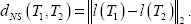
Abstract

When a phylogenetic reconstruction does not result in one tree but in several, tree metrics permit finding out how far the reconstructed trees are from one another. They also permit to assess the accuracy of a reconstruction if a true tree is known. TreeCmp implements eight metrics that can be calculated in polynomial time for arbitrary (not only bifurcating) trees: four for unrooted (Matching Split metric, which we have recently proposed, Robinson-Foulds, Path Difference, Quartet) and four for rooted trees (Matching Cluster, Robinson-Foulds cluster, Nodal Splitted and Triple). TreeCmp is the first implementation of Matching Split/Cluster metrics and the first efficient and convenient implementation of Nodal Splitted. It allows to compare relatively large trees. We provide an example of the application of TreeCmp to compare the accuracy of ten approaches to phylogenetic reconstruction with trees up to 5000 external nodes, using a measure of accuracy based on normalized similarity between trees.

Introduction

Different methods used to reconstruct phylogenetic trees often do not find the same tree for the same input data. This is because of the differences in their optimality criteria, in the way they search in the tree space (which is huge even for a relatively small number of taxa), and in their sensitivity to uncertainty in the input (usually nucleotide or protein sequences). Some methods (for example, maximum likelihood or maximum parsimony) often do not find one tree but a set of equally optimal trees, especially for a large number of external nodes (terminal nodes, leaves, often representing operational taxonomic units). Other methods, like Bayesian inference of trees, explicitly aim to find a set of trees: a sample from the posterior distribution of trees. Comparing the trees obtained using different methods or trees in a set obtained using one method requires a measure of distance between trees. Such measures (metrics for trees) are also useful when the accuracy of phylogenetic reconstruction methods is evaluated, in particular, when a new method is developed.^1,2 Other uses for tree metrics include tree comparison in mining phylogenetic information databases. ³

We have recently described some properties of a novel method for comparing unrooted phylogenetic trees, the Matching Split distance (MS). ⁴ Here we describe TreeCmp, a first implementation of this new metric and of its rooted version, the Matching Cluster distance (MC). TreeCmp also implements six other popular metrics for trees that can be computed in polynomial time: Robinson-Foulds (RF) ⁵ and a rooted version of RF based on clusters instead of splits (RC), Path Difference (PD), ⁶ Nodal Splitted with norm L ² (NS), ⁷ Triple (TT) ⁸ and Quartet (QT) ⁹ metric. Other metrics, for example, metrics based on edit operations, such as nearest neighbour interchange (NNI), subtree-pruning-regrafting (SPR) and Tree-Bisection-Reconnection (TBR), were not implemented in TreeCmp mainly because their computation is a non-deterministic polynomial-time hard (NP-hard) problem,^10–12 so their application is limited to small trees (with less than 100 external nodes). It is generally believed (but it has not been proven) that NP-hard problems do not have polynomial time (ie, computationally effective) solutions. All metrics implemented in TreeCmp take into account only the topology of compared trees. Branch lengths are ignored.

In this paper we present the new tool and an example of its application: we use TreeCmp to compare the accuracy of a set of popular reconstruction methods for unrooted trees with 250, 1250 and 5000 leaves.

Methods for Tree Comparison Implemented in TreeCmp

Since phylogenetic reconstructions sometimes do not allow to solve all multifurcations, TreeCmp implements distance measures for arbitrary (not only bifurcating) phylogenetic trees. Let U_L and R_L denote sets of all unrooted phylogenetic trees and all rooted phylogenetic trees over the set of leaves (species) L, respectively. All the distances implemented in TreeCmp are metrics over the sets U_L or R_L. A function d: X × X→R₊ ∪ {0} is a metric over X if and only if the following conditions are met: (i) for each x, y ∊ X, d(x, y) = 0 if and only if x = y, (ii) for each x, y∊X, d(x, y) = d(y, x), (iii) the triangle inequality: for each x, y, z∊X, d(x, y) + d(y, z) ≥ d(x, z). We will now describe briefly each metric implemented in TreeCmp and compare the distances obtained using each metric using 5-leaf unrooted (Fig. 1) or 4-leaf rooted trees (Fig. 2) as an example.

Figure 1

Computation of MS, RF, PD and QT distances for 5-leaf unrooted trees.

Figure 2

Computation of MC, RC, NS, and TT distances for rooted trees.

Matching Split metric (MS) for unrooted trees

MS ⁴ is based on comparing splits in two trees. A split A|B of a set L is an unordered pair (ie, A|B = B|A) of its subsets, such that L = A∩B and A∩B = Ø. Let min(A|B) = min{|A|, |B|}. To compare splits in two trees, MS finds a minimum-weight perfect matching in bipartite graphs whose vertices correspond to splits in these two trees and edges connect each split from one tree to a split in another tree. If the number of splits in the trees differs, the smaller set is extended by the missing number of “dummy” elements.

Because splits from the same tree are not linked in these graphs, these graphs are complete bipartite. One can chose a set of edges so that no two edges share a common vertex (such a set is called a matching) and so that every vertex is connected to another vertex (such a matching is called perfect). Many perfect matchings are possible for complete bipartite graphs. The one with the smallest total cost (sum of the weights associated with the edges) is minimal. The weight associated by MS to each edge is a measure of dissimilarity between splits: h_S(A|B, C|D) = min{|A⊕C|,|A⊕D|}, where X⊕Y = (X\Y)∪(Y\X) is a symmetric difference of the sets X and Y. For a “dummy” element O, h_S(A|B, O) = min{|A|,|B|}. The value h_S(A|B, C|D) is equal to the minimal number of leaf relocations needed to transform one split into the other. For example (Fig. 1), h_S(abc|de, acd|be) = 2, because 2 such relocations are needed: abc|de → ac|bde → acd|be. The cost h_S(A|B, O) can be interpreted as a cost of leaving an element A|B unmatched. MS distance between two unrooted phylogenetic trees T₁, T₂ ∊ U_L is the total cost of the minimal perfect matching between their splits. For unrooted trees in Figure 1, d_MS(T₁,T₂) = 3. The method allows also obtaining a matching (“alignment”) between their splits (red edges in Fig. 1).

Since the bipartite graphs for trees with n leaves can have at most 2(n – 3) vertices and the function h_S takes integer values, their perfect minimal matching can be found in time O(n^2.5logn) using methods described elsewhere.^13,14 Our implementation of MS uses another popular and effective algorithm, ¹⁵ which performs very well in practical applications. ¹⁶

Matching Cluster metric (MC) for rooted trees

To compare rooted trees, we define a metric similar to MS but which uses clusters instead of splits, the MC metric. A cluster associated with a vertex v in a rooted tree T with leaves L is a subset of leaves that are descendants of v. To measure the dissimilarity between clusters, MC uses function h_C(A, B) = |A⊕C|. For a dummy element, O = Ø, h_C(A, O) = |A|. For example, h_C(cd, abc) = 3. For rooted trees in Figure 2, d_MC(T₁,T₂) = 3.

MC inherits most of the features of MS, including computational complexity. In particular, an “alignment” between clusters of compared trees can be obtained at the same time as the distance is computed.

Robinson-Foulds metric (RF) for unrooted trees

The RF metric ⁵ is equal to the number of different splits in compared trees (divided by 2). It can be formulated in the same way as the MS metric, but replacing the function h_S with a simple function that returns 1 for different splits, 0 for identical splits, and 0.5 for unpaired (the distance to the “dummy” element). For unrooted trees in Figure 1, d_RF(T₁,T₁) = 2.

RF distance can be computed in O(n). ¹⁷ The implementation of RF in TreeCmp is slightly slower. We have optimized the comparison of splits (which are stored in a table as bit sets) using a hashing technique.

Robinson-Foulds metric based on clusters (RC) for rooted trees

Just as clusters can be matched instead of splits to formulate MC instead of MS, the function that is used to compare splits in RF can be used to compare clusters and to create the RC metric, so RC distance between trees is equal to the number of different clusters divided by 2. For rooted trees in Figure 2 d_RC(T₁,T₂) = 1.5. All implementations aspects are similar for RC and RF.

Path Difference metric (PD) for unrooted trees

Let e_ij(T) denote the number of edges in T∊U_n in the path joining leaves i and j, and let e(T) be the associated n(n – 1)/2-element vector obtained by a fixed ordering of the pairs {i, j}. Then the PD metric ⁶ between trees T₁, T₂ ∊ U_L is the square root of the sum of squared differences (e_ij(T₁) – e_ij(T₂)):

$$d_{PD}(T_1,T_2)={\Vert e(T_1)-e(T_2)\Vert }_2.$$

For unrooted trees in Figure 1, d_PD(T₁,T₂) = 14^1/2. The implementation of PD is based on calculation of distances between all pairs of leaves in time O(n ² ).

Nodal Splitted metric with norm L ² (NS) for rooted trees

While PD can be used only for unrooted trees, a family of metrics based on a similar principle (NS metrics) can be created for rooted trees. ⁷ Let l_T(i, j), denote the number of edges in T in the path joining leaf i with the most recent common ancestor of leaves i and j. For tree T ∊ R_L, (|L| = n) we define n × n square matrix l(T) as:

$$l(T)=\left(\begin{array}{cccc}0& l_T(\mathrm{1,2})& \cdots & l_T(1,n)\\ l_T(\mathrm{2,1})& 0& \cdots & l_T(2,n)\\ ⋮& ⋮& \ddots & ⋮\\ l_T(n,1)& l_T(n,2)& \cdots & 0\end{array}\right)$$

To make a NS metric similar to PD, one can use norm L ² to compare such matrices, with proven properties and advantages. ⁶ This is the norm we have implemented in TreeCmp. We thus define the NS distance between two trees T₁, T₂ ∊ R_L as:

$$d_{NS}(T_1,T_2)=\Vert l(T_1)-l(T_2){\Vert }_2.$$

For two rooted trees in Figure 2, d_NS(T₁,T₂) = 7^1/2. The implementation of NS in TreeCmp has time complexity O(n ² ).

Quartet metric (QT) for unrooted trees

The QT metric ⁹ is based on comparing sets of quartets induced by two trees. A set of quartets induced by an unrooted tree is the set of the topologies of all 4-species subsets of its leaves consistent with its topology. QT distance between two trees T₁, T₂ ∊ U_L is the number of different quartets in two respective sets. For two trees T₁ and T₂ presented in Figure 1, d_QT(T₁,T₂) = 4.

For bifurcating trees, QT can be computed in time O(nlogn). ¹⁸ For multifurcating trees, an algorithm with running time O(n^2.688) has been recently presented. ¹⁹ In TreeCmp we have modified and optimized the code form QuartetDist. ²⁰ The time complexity of this algorithm is O(n + |I‖I'|min{id, id′}), ²⁰ where id and id' are the degrees of internal nodes with the highest degree (disregarding edges to leaves) in two input trees (which may have multifurcations), and |I| and |I′| are the counts of internal (non-leaf) nodes. Therefore, the complexity varies between O(n ² ) for strictly bifurcating trees and O(n ³ ) in the worst case (eg, two different trees which both have internal nodes of degree n/2 linked to nodes which all connect to two leaves).

Triple metric (TT) for rooted trees

TT is similar to QT, but considers triples instead of quartets. A set of triples induced by a rooted tree is a set of the topologies of all 3-species rooted subtrees consistent with this tree. TT distance ⁸ between two trees T₁, T₂ ∊ R_L is the number of different triples in the respective sets. For two rooted trees T₁ and T₂ in Figure 2, d_TT(T₁,T₂) = 3.

The implementation of TT in TreeCmp is based on two algorithms, both with time complexity O(n ² ). In the case of bifurcating trees, a well-known and relatively old algorithm is used. ⁸ For non-bifurcating trees, TreeCmp is using a newer and much more complicated algorithm. ²¹

Topological accuracy measure based on normalized similarity between trees

In ¹ the topological accuracy (TA) is defined as the proportion of the splits in the true tree that are recovered by a given phylogenetic reconstruction method. This measure of TA is based explicitly on RF. We have created a more general measure of topological accuracy according to a particular metric m (TA_m), based on normalized tree similarity for a particular metric (NTS_m).

Distances between random trees (for example, generated using the Yule method ²² ) grow with the number of leaves for all metrics considered here (Table 1; the maximum distances in the space of trees also grow, but are less useful as scaling factors). To allow for comparison of distances for trees with different number of trees, NTS_m compares the distance with the average distance between random trees $\overline{d}$ _{m, rand} obtained using the same metric (Table 1):

Table 1

The average distance and computation time for random and similar trees using metrics implemented in TreeCmp.

Metric	Trees with 250 leaves			Trees with 1250 leaves			Trees with 5000 leaves
	Average distance between random trees	Comp. time for random trees [ms]	Comp. time for similar trees [ms]	Average distance between random trees	Comp. time for random trees [ms]	Comp. time for similar trees [ms]	Average distance between random trees	Comp. time for random trees [ms]	Comp. time for similar trees [ms]
MS	2939.20	12.2	2.16	22606.81	248.37	22.4	118474.06	6287.87	565.1
MC	3254.05	19.66	2.90	24155.17	286.27	28.30	126018.21	8644.62	549.04
RF	246.78	2.3	1.72	1246.78	4.21	8.3	4996.78	18.34	45.0
RC	247.86	4.79	2.40	1247.77	9.14	14.86	4997.72	69.52	81.20
PD	1112.62	3.19	5.11	6608.38	40.82	60.59	29197.47	1051.81	1548.61
NS	1312.09	4.57	2.88	7435.33	32.85	30.31	31896.02	892.47	620.93
QT	1.059E08	86.82	76.59	6.749E10	2234.11	2129.4	1.734E13	39711.04	40710.0
TT	1.713E06	9.84	5.83	2.166E08	99.78	131.69	1.389E10	2179.69	2143.55

Notes: Average distances between random trees generated using the Yule method was calculated for 10,000 pairs of unrooted (MS, RF, PD, QT) and 100 pairs of rooted (MC, RC, ND, TT) trees. Average computational time per tree is based on 100 comparisons for random trees, 3080 comparisons for similar trees with 250 leaves (calculating the distance between the true tree and the trees reconstructed for 308 alignments using 10 methods), 784 comparisons for 1250 leaves (92 alignments, 8 methods), and 56 comparisons for 5000 leaves (7 alignments, 8 methods). The first leaf was used as outgroup when rooting the trees.

$$NT{S}_m(T_1,T_2)=\frac{{\overline{d}}_{m,rand}-d_m(T_1,T_2)}{{\overline{d}}_{m,rand}}.$$

NTS_m is 1 when distance between two trees is 0 (both trees are the same), and is about 0 when the trees are as similar (according to a given metric) as two random trees on average. NTS_m (T₁,T₂) < 0 when T₁ and T₂ are further apart than two random trees.

When one of the trees is a true tree (T*) and the other is reconstructed (T_r), NTS_m is a measure of topological accuracy of the reconstruction: TA_m = NTS_m (T*,T_r). The model we have used to generate random trees (the Yule model) assumes instantaneous, strictly bifurcating speciation occurring with the same probability for all lineages at any given time. ²² Trees are constructed iteratively: starting from four random taxa, new taxa (chosen randomly) are added to a branch connected to a leaf. ²² As the size of trees goes to infinity, RF distance for two Yule random trees follows asymptotically the Poisson distribution, and the average value quickly tends to the number of non-trivial splits, ⁶ so TA_RF is very close to the measure of proportion of true splits used in. ¹

Using Metrics Implemented in TreeTmp to Compare Trees

The comparison of phylogenetic trees is a difficult problem, and even very intuitive measures may lead to non-intuitive results. Consider three trees with five leaves presented in Figure 3. Which of the two trees T₁ or T₃ is the most similar to T₂? According to the RF metric, both trees are equally similar to T₂. However, all other metrics indicate that T₁ and T₂ are more similar than T₂ and T₃ The second answer is more intuitive, because removing leaf e makes trees T₁ and T₂ identical, while there is no similar operation for trees T₂ and T₃.

Figure 3

Distances between trees with 5 leaves and normalized tree similarities between “caterpillar trees” using different metrics.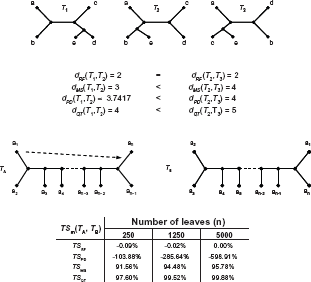

MS can be regarded as a refinement of RF, so these two metrics are the easiest to compare. MS takes into account not only the identity of splits, but also more subtle similarities, so for any set of trees it gives a wider range of distance values, allowing for improved diversification. In comparison to RF, MS concentrates more on differences corresponding to edges deep inside the tree (when both parts of a split A|B have large cardinality) than on differences corresponding to edges closer to the leaves. Finally, MS allows for structural comparison of trees by returning an optimal matching between their splits.

The fundamental advantage of MS over RF is that for large phylogenies, relocations of a bounded number of leaves cause small changes of MS distances (O(n), asymptotically small in comparison to Θ(n ² ) for maximal possible MS distance for n-leaf trees). In contrast, RF distance can increase from 0 to the maximal value for a given number of leaves after only one relocation of a single leaf (a₁) in a “caterpillar” tree (Fig. 3). The normalized relative similarity between two such “caterpillar” trees varies hugely depending on which metric is used. For RF and PD, a large discrepancy is observed (average NTS_RF around 0% and NTS_PD less than 0%). MS and QT suggest high similarity (NTS_MS and NTS_QT over 90%, and increasing as the trees grow larger). The results given by MS and QT are more intuitive.

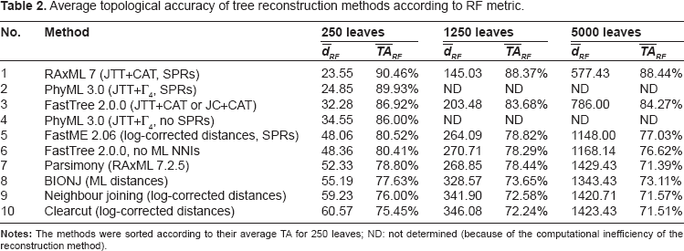
To investigate what effect different properties of metrics for unrooted trees can have for phylogenetic trees reconstructed using biological sequences, we have used 3 previously described data sets ¹ of simulated protein alignments (see ¹ for details; these data sets are available at http://microbesonline.org/fasttree/#Sims). We have obtained the average topological accuracy (for 308 different sequence alignments with 250 sequences, 92 with 1250 sequences, and 7 with 5000 sequences) of 10 approaches to phylogenetic reconstruction: RAxML 7 ²³ with SPR, PhyML 3^24,25 with SPR or without, BIONJ ²⁶ with ML distances obtained using PROTDIST (part of PHYLIP ²⁷ ), FastTree 2 ¹ with Maximum Likelihood NNI to improve the tree or only minimum-evolution SPR (no ML NNIs), FastME 2, ²⁸ Parsimony (using RAxML 7.2.5), neighbour joining, ²⁹ and its faster variant Clearcut. ³⁰ JTT model ³¹ (using 4 rate categories in the Γ distribution or the CAT approximation which estimates the rate for each site, see ¹ for details) or log-corrected distances were used to measure evolutionary distances between sequences.

Different metrics for unrooted trees agree in general on the ranking of 10 approaches to phylogenetic reconstructions compared here (Tables 2–5): the order is the same for positions 1–4 and 9–10. However, the ordering of BIONJ, FastTree 2.0.0 (no ML NNIs), FastME and Parsimony differs, with some interesting patters. First of all, all metrics agree that Parsimony has the worst accuracy among these 4 reconstruction methods for very large trees (5000 leaves). Secondly, MS, QT and PD (with the exception of 1250 leaves), but not RF, agree that BIONJ has the best accuracy among 4. Thirdly, and again with one exception (QT and 5000 leaves), 3 metrics but RF agree that the accuracy of FastTree 2.0.0 without ML NNIs is higher than the accuracy of FastME.

Table 2

Average topological accuracy of tree reconstruction methods according to RF metric.

No.	Method	250 leaves		1250 leaves		5000 leaves
		$\overline{d}$ RF	$\overline{T}\overline{A}$ RF	$\overline{d}$ RF	$\overline{T}\overline{A}$ RF	$\overline{d}$ RF	$\overline{T}\overline{A}$ RF
1	RAxML 7 (JTT+CAT, SPRs)	23.55	90.46%	145.03	88.37%	577.43	88.44%
2	PhyML 3.0 (JTT+Γ4, SPRs)	24.85	89.93%	ND	ND	ND	ND
3	FastTree 2.0.0 (JTT+CAT or JC+CAT)	32.28	86.92%	203.48	83.68%	786.00	84.27%
4	PhyML 3.0 (JTT+Γ4, no SPRs)	34.55	86.00%	ND	ND	ND	ND
5	FastME 2.06 (log-corrected distances, SPRs)	48.06	80.52%	264.09	78.82%	1148.00	77.03%
6	FastTree 2.0.0, no ML NNIs	48.36	80.41%	270.71	78.29%	1168.14	76.62%
7	Parsimony (RAxML 7.2.5)	52.33	78.80%	268.85	78.44%	1429.43	71.39%
8	BIONJ (ML distances)	55.19	77.63%	328.57	73.65%	1343.43	73.11%
9	Neighbour joining (log-corrected distances)	59.23	76.00%	341.90	72.58%	1420.71	71.57%
10	Clearcut (log-corrected distances)	60.57	75.45%	346.08	72.24%	1423.43	71.51%

Notes: The methods were sorted according to their average TA for 250 leaves; ND: not determined (because of the computational inefficiency of the reconstruction method).

Table 3

Average topological accuracy of tree reconstruction methods according to PD metric.

No.	Method	250 leaves		1250 leaves		5000 leaves
		$\overline{d}$ PD	$\overline{T}\overline{A}$ PD	$\overline{d}$ PD	$\overline{T}\overline{A}$ PD	$\overline{d}$ PD	$\overline{T}\overline{A}$ PD
1	RAxML 7 (JTT+CAT, SPRs)	245.42	77.94%	1982.16	70.01%	10844.37	62.86%
2	PhyML 3.0 (JTT+Γ4, SPRs)	254.38	77.14%	ND	ND	ND	ND
3	FastTree 2.0.0 (JTT+CAT or JC+CAT)	303.92	72.68%	2603.88	60.60%	17695.31	39.39%
4	PhyML 3.0 (JTT+Γ4, no SPRs)	325.41	70.75%	ND	ND	ND	ND
5	BIONJ (ML distances)	438.70	60.57%	3326.51	49.66%	14568.16	50.10%
6	FastTree 2.0.0, no ML NNIs	440.38	60.42%	3243.49	50.92%	14911.68	48.93%
7	FastME 2.06 (log-corrected distances, SPRs)	449.37	59.61%	3420.10	48.25%	15563.98	46.69%
8	Parsimony (RAxML 7.2.5)	452.24	59.35%	3284.08	50.30%	18126.62	37.92%
9	Neighbour joining (log-corrected distances)	483.03	56.59%	3749.12	43.27%	16207.15	44.49%
10	Clearcut (log-corrected distances)	541.15	51.36%	3927.25	40.57%	15842.29	45.74%

Notes: The methods were sorted according to their average TA for 250 leaves; ND: not determined (because of the computational inefficiency of the reconstruction method).

Table 4

Average topological accuracy of tree reconstruction methods according to MS metric.

No.	Method	250 leaves		1250 leaves		5000 leaves
		$\overline{d}$ MS	$\overline{T}\overline{A}$ MS	$\overline{d}$ MS	$\overline{T}\overline{A}$ MS	$\overline{d}$ MS	$\overline{T}\overline{A}$ MS
1	RAxML 7 (JTT+CAT, SPRs)	222.98	92.41%	2256.15	90.02%	12410.00	89.53%
2	PhyML 3.0 (JTT+Γ4, SPRs)	234.31	92.03%	ND	ND	ND	ND
3	FastTree 2.0.0 (JTT+CAT or JC+CAT)	293.95	90.00%	3325.75	85.29%	19830.43	83.26%
4	PhyML 3.0 (JTT+Γ4, no SPRs)	313.62	89.33%	ND	ND	ND	ND
5	BIONJ (ML distances)	482.04	83.60%	4418.58	80.45%	20555.43	82.65%
6	FastTree 2.0.0, no ML NNIs	499.15	83.02%	4402.59	80.53%	23219.14	80.40%
7	Parsimony (RAxML 7.2.5)	510.11	82.64%	4418.33	80.46%	27135.71	77.10%
8	FastME 2.06 (log-corrected distances, SPRs)	510.89	82.62%	4501.62	80.09%	23796.00	79.91%
9	Neighbour joining (log-corrected distances)	556.27	81.07%	5086.80	77.50%	25391.57	78.57%
10	Clearcut (log-corrected distances)	610.25	79.24%	5183.72	77.07%	25276.86	78.66%

Notes: The methods were sorted according to their average TA for 250 leaves; ND: not determined (because of the computational inefficiency of the reconstruction method).

Table 5

Average topological accuracy of tree reconstruction methods according to QT metric.

No.	Method	250 leaves		1250 leaves		5000 leaves
		$\overline{d}$ QT	$\overline{T}\overline{A}$ QT	$\overline{d}$ QT	$\overline{T}\overline{A}$ QT	$\overline{d}$ QT	$\overline{T}\overline{A}$ QT
1	RAxML 7 (JTTCAT, SPRs)	4.352E06	95.89%	5.671E09	91.60%	1.752E12	89.90%
2	PhyML 3.0 (JTT Γ4, SPRs)	4.762E06	95.50%	ND	ND	ND	ND
3	FastTree 2.0.0 (JTTCAT or JCCAT)	8.162E06	92.29%	1.012E10	85.01%	2.872E12	83.44%
4	PhyML 3.0 (JTT Γ4, no SPRs)	8.863E06	91.63%	ND	ND	ND	ND
5	BIONJ (ML distances)	1.401E07	86.77%	1.300E10	80.74%	2.889E12	83.34%
6	Parsimony (RAxML 7.2.5)	1.567E07	85.21%	1.393E10	79.36%	5.469E12	68.46%
7	FastTree 2.0.0, no ML NNIs	1.635E07	84.56%	1.458E10	78.39%	4.480E12	74.16%
8	FastME 2.06 (log-corrected distances, SPRs)	1.695E07	83.99%	1.506E10	77.68%	3.939E12	77.28%
9	Neighbour joining (log-corrected distances)	1.808E07	82.93%	1.639E10	75.71%	4.940E12	71.51%
10	Clearcut (log-corrected distances)	1.946E07	81.63%	1.641E10	75.69%	4.938E12	71.53%

Notes: The methods were sorted according to their average TA for 250 leaves; ND: not determined (because of the computational inefficiency of the reconstruction method).

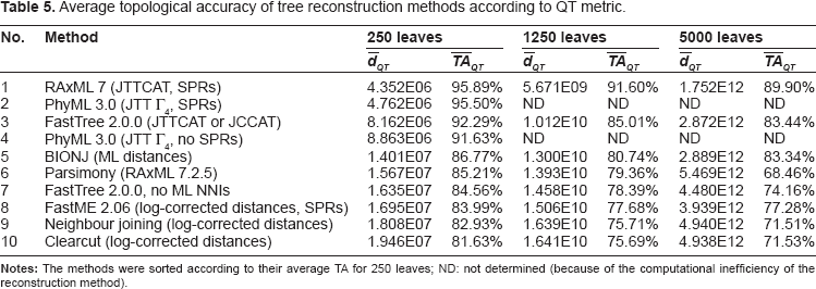
Another observation concerns the fact that according to PD, the reconstructed trees are further away from the true tree relative to the average distance between random trees, than according to the other 3 metrics. In other words, the values of average topological accuracy according to PD are, in general, much lower than for the other metrics, their range is 37.92%–77.94% compared with 71.39%–90.46% for RF, 77.10%–92.41% for MS, and for 68.46%–95.89% (Tables 2–5). This measure also indicates that as the number of leaves increases, the topological accuracy of FastTree and Parsimony reconstructions is more affected than the accuracy of other methods.

The calculation of distances between random trees generated using the Yule process allows to compare the running time for distance calculation using TreeCmp (Fig. 4). Not surprisingly, the calculation of distances was the fastest for RF, and the slowest for QT. PD could be computed faster than MS. The calculation of average TA_m requires the comparison of true trees and trees reconstructed by a particular method for a particular alignment, so we could compare the running times for calculations of distances between random trees with the times for similar trees (Table 1). Computation time of MS in case of trees that share some splits can be optimized considerably because the shared splits can be omitted from further computation. ⁴ This results in reducing the size of the bipartite graph used for computing the minimum-weight prefect matching. In consequence, MS can be computed one order of magnitude faster for simulated trees with 5000 leaves than for random trees.

Figure 4

Computation time of distances between trees using TreeCmp for different metrics.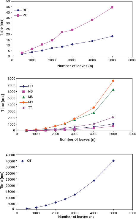

Finally, it is easy to obtain normalized distances using normalized similarity for a given metric: δ_m = 1 – NTS_m. A normalized distance larger than one indicates that two trees are more dissimilar than two random trees with the same number of leaves according to a given metric. Such normalization provides more intuitive measures of tree similarity than the original metrics, measures that are stable as the number of leaves increases.

Availability, System Requirements, User Interface, and Comparison with other Software

We have created TreeCmp as a stand-alone application in Java with a command line interface and a system of hints built on base of Jakarta Commons CLI. The application is freely available at http://kaims.pl/~dambo/treecmp/.

TreeCmp takes as input a file with N > 2 trees and allows for: sequential pairwise comparison (command line option: -s; the output is N – 1 distances between pairs of trees neighbouring in the list), sequential window comparison (-w <window size S>; the output is distances between all trees in neighbouring non-overlapping windows), all-to-all pairwise comparison (-m; the output is N(N – 1)/2 pairwise distances between trees), and one-to-all comparison (-r <file with one reference tree>; each tree in the input file is compared to the reference tree).

In addition, TreeCmp allows for comparison of trees with different leaf sets (–P). Since all the implemented metrics take as input two trees on the same set of leaves, trees on different leaf set are pruned to subtrees having the same set of leaves. Then the subtrees are compared using selected metrics.

We have also allowed for reporting of distances (-N) scaled by the average distance between two random trees with the same number of leaves (see below for the discussion of these scaled metrics). After enabling this option two additional columns per each chosen metric appears in the output file (for two different tree generation methods; the Yule model and the uniform model; see ²² for review). The software uses pre-computed values of averages stored in 16 files (for 8 metrics and 2 random tree generation methods). The files contain also standard deviations and quantiles, so they can be used to test the null hypothesis that the distance between two given trees in not larger than the average distance between random trees with the same number of leaves.^6,32

Another feature implemented in TreeCmp is the generation of an “alignment” between trees (-A). A side effect of MS/MC metric computation is a perfect matching that illustrates best correspondence between edges (or nodes) in both trees. Because a perfect matching with minimal weight is not necessarily unique, this matching of similar splits (for MS) or clusters (for MC) is also not unique. However, identification of corresponding phylogenetic groups may be useful for the analysis of large phylogenies, so this method could be an alternative to or extension of software tools for this purpose (eg, TreeJuxtaposer ³³ ).

TreeCmp has a very general input file parser based on PAL. ³⁴ The application simply searches for trees in the Newick format (a sequence of characters that begins with the left parenthesis and ends with the right parenthesis and a semicolon), so files created by commonly used phylogenetic packages (MrBayes, BEAST, PAUP, PHYLIP) are supported without any pre-processing.

Output files are tab separated text files (TSV). Such files can be easily read by various data analysis software packages (for example R, Microsoft Excel, OpenOffice.org). The content of an output can file consists of two sections. The first section contains distances using selected metrics. The second optional section (enabled using –I switch) contains some general statistics for all rows in the first section (row average and standard deviation, minimal and maximal values).

As far as we are aware, there is no other software which would allow computing the MC/MS distance or would conveniently implement the NS metric (the only other implementation ⁷ is in pre-release and requires knowledge of Python). However, there are several free tools for computing subsets of popular tree metrics. One such tool is COMPONENT 2.0 ³⁵ which allows to compute RF, TT, and QT distances (and to perform many other operations on phylogenetic trees). Unfortunately, using COMPONENT 2.0 we were unable to compare trees with more than 100 leaves. Another tool, TOPD/FMTS, ³⁶ allows computing RF, PD, QT, and TT, but is considerably slower than TreeCmp. For example, comparison of two unrooted trees takes 2 min for 5000 leaves using RF metric (and <1 s with TreeCmp), >1 h for 1250 leaves using PD (< 1 s with TreeCmp) and >20 h for 100 leaves using QT (< 1 s with TreeCmp). Comparison of rooted trees for 100 leaves using TT metric takes >30 min (< 1 s with TreeCmp). All the tests have been performed on Intel Core i7 920 2.66 GHz with 12 GB RAM server under Ubuntu 10.10.

Conclusions

We provide a tool, TreeCmp, that allows to efficiently compare relatively large (even up to 5000 leaves) arbitrary (possibly multifurcating) trees using four measures for unrooted and four measures for rooted trees. Other available software tools are much more limited: they often implement a small number of measures and are computationally inefficient (in particular, they do not allow comparing large trees). TreeCmp is the first implementation of the Matching Split metric and its rooted variant, the Matching Cluster metric. The computation of these two metrics permits to obtain the alignment of splits (or clusters) in two trees using TreeCmp. The tool also provides a modified, optimized implementation of the Quartet metric adopted form, ²⁰ an efficient version of the Triple metric, a version of the Robinson-Foulds metric, implemented using bit sets and hashing technique, together with its rooted variant based on clusters. Finally, TreeCmp provides an efficient implementation of the Path Difference and Nodal Splitted metrics. The software calculates normalized distances between trees for all the metrics that have been implemented (for trees with 4-1000 leaves). We believe that such normalized distances are more intuitive measures of dissimilarity between trees. Since the tool is written in Java, TreeCmp is ready to run on a variety of operating systems without installation or compilation. We show that four metrics for unrooted trees implemented in TreeCmp may give different results when assessing the accuracy of phylogenetic reconstruction. When such a situation takes place, it is the results obtained with Robinson-Foulds metric that usually do not agree with the other three metrics (Matching Split, Path Difference and Quartet).

List of Abbreviations

MC

the Matching Cluster metric for rooted trees;

MS

the Matching Split metric for unrooted trees;

NNI

a metric based on nearest neighbour interchange operations;

NP-hard

a class of non-deterministic polynomial-time hard problems;

NS

the Nodal Splitted metric with norm L ² for rooted trees;

NTS _m

normalized similarity between trees for a particular metric m;

PD

the Path Difference metric for unrooted trees;

QT

the Quartet Metric for unrooted trees;

RC

the Robinson-Foulds metric based on clusters for rooted trees;

RF

the Robinson-Foulds metric for unrooted trees;

SPR

a metric based on subtree prune and regraft operations;

TA _m

Topological Accuracy of a tree reconstruction according to metric m;

TBR

a metric based on tree bisection and reconnection operations;

TT

the Triple Metric for rooted trees.

Author Contributions

Implemented distance metrics in TreeCmp, carried out the numerical analysis: DB. Participated in designing the algorithms: KG. Conceived and designed the study, analysed the results, and prepared the manuscript: BW. All authors reviewed and approved of the final manuscript.

Funding

This work was supported by the Polish Ministry of Science and Education (grant number N303 291234 to BW), and the Polish National Science Centre (decision number DEC-2011/02/A/ST6/00201 to KG and DB).

Competing Interests

Author(s) disclose no potential conflicts of interest.