Model-Integrated Estimation of Normal Tissue Contamination for Cancer SNP Allelic Copy Number Data

Abstract

SNP allelic copy number data provides intensity measurements for the two different alleles separately. We present a method that estimates the number of copies of each allele at each SNP position, using a continuous-index hidden Markov model. The method is especially suited for cancer data, since it includes the fraction of normal tissue contamination, often present when studying data from cancer tumors, into the model. The continuous-index structure takes into account the distances between the SNPs, and is thereby appropriate also when SNPs are unequally spaced. In a simulation study we show that the method performs favorably compared to previous methods even with as much as 70% normal contamination. We also provide results from applications to clinical data produced using the Affymetrix genome-wide SNP 6.0 platform.

1. Introduction

DNA in tumor cells can contain abnormalities in the form of copy number aberrations such as segments with losses or gains of one or several copies of either allele. The lengths of such aberrations can vary between short segments up to an entire chromosome, and their positions are essential both for detecting and for improving knowledge of various sorts of cancer. Therefore, methods that localize copy number aberrations are of great importance. In addition to changes in the total copy number of both alleles together, changes in the allelic copy numbers, ie, the number of copies of each allele, are also important. We denote the two different alleles at a given genomic location by A and B, so that for normal cells the possible genotypes are AA, AB and BB. One example of a genotype aberration is loss of heterozygosity (LOH), for which the only attainable genotypes are AA and BB.

Different techniques to measure DNA copy numbers have been developed, as have methods to evaluate the measurement data. One technique is array comparative genomic hybridization (aCGH), which provides ratios of the copy numbers of a sample DNA, compared to those of some reference DNA. Several different statistical methods have been applied to this kind of data, including different segmentation methods,^4,20,21 smoothing^6,12 and hidden Markov models.^{1,7,9,16,19,24,27,28,29} aCGH data provides information only about the total copy number and gives no information about the amount of each allele. Another drawback with such data is the limited number of probes on the arrays. For this reason there is an increased use of single nucleotide polymorphism (SNP) data, which offers denser measurements and provides intensities for the two alleles separately. Using SNP data it is possible not only to estimate copy number changes, but also to find allelic changes such as LOH. Indeed, a copy number amplification may be caused by different allelic changes. For example, a copy number of four could correspond either to {AAAA, AAAB, ABBB, BBBB}, to {AAAA, AABB, BBBB} or to {AAAA, BBBB}, depending on which allele that has gained extra copies.

SNP data has previously been analyzed using various sorts of methods, such as smoothing^11,15 and pattern recognition. ²² The most frequently used methods are however based on hidden Markov models (HMMs).^{3,8,13,17,18,26,30,31} A brief introduction to Markov chains and HMMs is found in Appendix 1. HMMs suit SNP data well since genomic alterations often appear in longer or shorter segments, implying that copy numbers across probes in a small genomic region are correlated. For example, Wang et al ³¹ and Colella et al ³ model SNP data from the Illumina array, which provides log R ratio data (log₂-ratio of total observed intensities to total expected intensities) and BAF data (normalized measure of the relative intensities of the two alleles), using an HMM with six states, while Sun et al ³⁰ apply a more comprehensive model with nine states. Korn et al ¹³ combine an HMM to model copy number variants with a clustering algorithm to detect genotypes. Li et al ¹⁸ also model the proportion of the major allele while Lamy et al ¹⁷ use both allelic intensities provided by the Affymetrix array and model them using bivariate Normal distributions.

Several of the methods above assume that the ploidy, ie, mean copy number, of a chromosome is two. This holds for normal cells, but cancer cells are anueploid, ie, their ploidy may differ from two. The necessity for considering ploidy when modeling cancer data is well described by Greenman et al, ⁸ but in brief one can say that the measured normalized intensity for a probe in a diploid chromosome is twice as large as for a probe with the same copy number in a quadroploid chromosome. Two methods that include ploidy are those of Attiyeh et al ² and Greenman et al, ⁸ which both contain a pre-processing step in which the ploidy is estimated. Greenman et al then continue by using an HMM while Attiyeh et al apply a window-based model.

Another feature common in tumor samples, arising from the difficulty to dissect tumor cells only from a tissue sample, is contamination of the tumor cell sample by normal cells. As a result the measured allelic intensities are mixtures of intensities from tumor and normal cells, thus yielding non-integer DNA copy numbers. One way to incorporate such contamination is to model total copy numbers of the mixed sample in a non-parametric way,^2,29 but this provides limited information about the copy numbers of the cancer cells. Sun et al ³⁰ estimate the fraction of normal tissue contamination using an empirical method and Colella et al ³ write that it is possible to extend their method to handle contamination, but without being more specific. Li et al ¹⁸ show that their method can handle a fraction of normal tissue contamination up to 30%, while Lamy et al ¹⁷ report a simulation study with slightly better results. Some tumors however form in a manner such that even with microdisection, a significant proportion of normal cells (say 50% or more) can arise in the sample, and none of the above methods provide results that are satisfactory for such high fractions of normal tissue contamination.

The purpose of the present paper is to devise a method to estimate allelic copy numbers, with ploidy and fraction of normal tissue contamination integrated in the model. Indeed, in all of the above papers, ploidy and/or normal fraction are estimated by adding more or less ad-hoc steps to a model that does not account for these parameters in itself. The model reported here is thus particularly suited for cancer data, for which both of these features are common. By including these parameters in the model they can be estimated alongside the other parameters using all data, rather than adding a pre-processing step or empirical methods using only a small subset of the data. In the simulation study presented below, samples with 30%, 50% and 70% normal contamination are simulated and even for the largest amount of contamination, 97% of the probes are reconstructed to the correct copy number state.

An additional feature of our model is that it is based on a continuous-index Markov chain, which accounts for the fact that the SNP probes are often unevenly spread over the genome. The relevance of a continuous-index model was highlighted by Gupta and Mitra ¹⁰ (Section 5.3) for the different but related problem of classifying regions of DNA as nucleosome free regions (NFR) or non-NFR using a two-state HMM. Indeed, they showed that with irregularly spaced probes, a continuous-index model can provide substantially better results than a discrete-index model; 99% vs. 85% or 68% correct classifications in simulations for two different arrangements of the probes. Also the methods by Wang et al, ³¹ Colella et al ³ and Li et al, ¹⁸ who apply discrete-index HMMs to SNP data, aim to take distances between probes into account by letting the Markov transition probabilities depend on these distances in different ways. Common to all of these methods is however that the stipulated transition probabilities violate the Chapman-Kolmogorov equation of Markov chains. That is, letting P(t) be the matrix of transition probabilities over a distance t between two probes, the equality P(t₁ + t₂) = P(t₁)P(t₂) does not hold. In essence this means that there is in fact no Markov chain with the given transition probabilities.

The paper is organized as follows. The model is described in in Section 3. Section 4 provides results from a simulation study as well as from an application to clinical data. Concluding remarks are given in Section 5.

2. Data

The data used in this study are the cancer samples in Greenman et al, ⁸ produced using the Affymetrix genome-wide SNP 6.0 platform. We applied the algorithm to about 15 different cell line and primary tumor samples, representing various cancer forms including breast, lung and renal cancer. The primary tumor sample PD1753a for which results are reported in Section 4.2 are from a clear cell renal cell carcinoma sample. ³²

For probes at SNPs the intensities of the two different alleles are provided, while at other positions only a single total copy number intensity is available. Following Greenman et al, ⁸ the intensities are normalized by first dividing each measurement by the total intensity of the sample (ie, the sum of all probe intensities over the entire genome), to remove chip-to-chip variation. The mean signals for each allele (or probe at non-SNP positions) are then transformed into a copy number intensity and a genotype intensity that are indicators of total copy number and allelic ratio dosages. The model presented below incorporates intensities for SNP probes only, but is easily extendable to include also probes measuring total copy number only; we elaborate on this further in the Discussion. The cancer data is available from the Cancer Genome Project, subject to a manual transfer agreement, and our Matlab code is available on the WWW. ³³

3. The Model

3.1. Basic structure

Let there be N_c probes on chromosome c, and denote these probes as probe (k, c), k = 1, 2, …, N_c. The genomic location of probe (k, c) is denoted by t _kc , measured in the unit base pairs (bp) starting from the beginning of the chromosome. We denote the two different alleles at any genomic location by A and B. We will write g = (g_A, g_B) for the allelic copy numbers, ie, g_A and g_B are the number of copies of the A and B allele respectively. For example, the genotype AAB corresponds to g = (2, 1). Obviously the genotype and the allelic copy numbers are in a one-to-one correspondence to each other, and at times we will make no real distinction between the two. The allelic intensities are modeled using an HMM for which each state i corresponds to one genotype set G _i as specified in Table 1. The Markov chain can be extended to include more states with copy numbers above six, but the model as stated here has proved to be enough for the studied samples. To explain the genotype sets in Table 1, we note that through cancer development any region in the genome starts with one parental copy of each region and ends up with m copies of one allele and n copies of the other. If the genotype was originally AA or BB then the genotype will be (m + n) A or (m + n)B, respectively. If the SNP was heterozygous then we must end up with either mA and nB, or mB and nA. These are the genotypes indicated in Table 1. We refer to state 4, with genotype set {AA, AB, BB} as the normal state, and by an abnormal state we mean any other state.

Table 1.

Genotype sets for the different states of the Markov chain, sorted in the order given by the total copy number and copy number of the minor allele.

State i	(Total CN, minor CN)	Genotype set G i
1	(0,0)	{}
2	(1,0)	{A, B}
3	(2,0)	{AA, BB}
4	(2,1)	{AA, AB, BB}
5	(3,0)	{AAA, BBB}
6	(3,1)	{AAA, AAB, ABB, BBB}
7	(4,0)	{4A, 4B}
8	(4,1)	{4A, 3AB, A3B, 4B}
9	(4,2)	{4A, 2A2B, 4B}
10	(5,0)	{5A, 5B}
11	(5,1)	{5A, 4AB, A4B, 5B}
12	(5,2)	{5A, 3A2B, 2A3B, 5B}
13	(6,0)	{6A, 6B}
14	(6,1)	{6A, 5AB, A5B, 6B}
15	(6,2)	{6A, 4A2B, 2A4B, 6B}
16	(6,3)	{6A, 3A3B, 6B}

For each chromosome c the sequence of copy number states, according to Table 1, is modeled by a continuous-index Markov chain ${\left(X_c\left(t\right)\right)}_{t_{1c}\le t\le T_c}$ , where t and T _c are respectively the genomic location (in bp) within the chromosome and the length (in bp) of the chromosome. The Markov chains for different chromosomes are assumed independent. The genomic location (in bp) is, strictly speaking, a discrete variable, but since the number of bp's within a chromosome is much larger than the number of jumps of the Markov chain, the error caused by using a continuous approximation is negligible. With a discrete-index model the Markov transition probabilities would either be very close to unity (for staying in the same state from one bp to another) or close to zero (for changing state), and dealing with such probabilities is unstable numerically. For a continuous-index model, using transition rates rather than probabilities, this problem does not exist.

With 16 different states there are 240 different types of jumps and equally many transition rates (per chromosome). It is infeasible to estimate such many rates, and to make the model more parsimonious we assume a large number of them to agree. Specifically we assume, for chromosome c, a common rate λ _c for jumps from any state (normal or abnormal) to the group of abnormal states, with each such state, except for the current one in case the chain resides in an abnormal state, being equally likely, and another common rate η _c for jumps to the normal state from any abnormal state. The total rate out of any abnormal state, for chromosome c, is thus ${\lambda }_c+{\eta }_c$ . This dynamic provides Markov chains whose stationary versions are time-reversible. ²⁹ Finally we let ${\delta }_{ic}=P\left(X_c\left(t_{1c}\right)=i\right)$ denote the initial probability for Markov state i in chromosome c.

Write y _kc = (y_Akc, y_Bkc) for the measured allelic intensities at probe (k, c). Greenman et al ⁸ studied the correlation between the allele A and B intensities, for each probe, using 460 wild-type samples. For probe (k, c), plotting the two allele intensities for all wild-type samples against each other reveals three clusters (see, ⁸ Figure 1, for an example). These clusters correspond to the genotypes AA, AB and BB, with the coordinates of the cluster centers written as (A_0kc + 2A_1kc, B_0kc), (A_0kc + A_1kc, B_0kc + B_1kc) and (A_0kc, B_0kc + 2B_1kc) respectively for suitable parameters A_0kc, B_0kc, A_1kc and B_1kc These parameters were all estimated by Greenman et al ⁸ using the wild-type samples. Their interpretation is that A_0kc is the background intensity of the A allele (at diploid probes BB), and A_1kc is the increase in A allele intensity from BB to AB and from AB to AA; B_0kc and B_1kc have analogous interpretations.

Figure 1.

Proportions of probes at which the Markov state was incorrectly reconstructed by the Viterbi algorithm with MAP parameter estimates computed by the EM algorithm. Markov transition rates were λ _c = η _c = 10^–7 (top left), λ _c = 10^–7, η _c = 10^–9 (top right), λ _c = 10^–9, η _c = 10^–7 (bottom left), λ _c = η _c = 10^–9 (bottom right) (unit: bp^–1). Confidence intervals were obtained by exponentiating two-sided 95% student-t confidence limits based on the log-proportions for 10 genome replicates.

Further denote by ( ${\mu }_{\text{A}kcg},{\mu }_{\text{B}kcg}$ ) the mean allele A and B intensities at probe (k, c) for allelic copy numbers g = (g_A, g_B). The cluster centers above then write

$$\begin{array}{c}{\mu }_{kcg}=\left({\mu }_{\text{A}kcg},{\mu }_{\text{B}kcg}\right)\\ =\left(A_{0kc}+g_{\text{A}}{A}_{1kc},B_{0kc}+g_B{B}_{1kc}\right),\end{array}$$

(1)

and this model applies for the normal Markov state i = 4, ie, for allelic copy numbers such that g_A + g_B = 2. Moreover, the clusters in Greenman et al ⁸ (Fig. 1) are tilted ovals, indicating that the intensities for alleles A and B are correlated and have unequal variances. Greenman et al ⁸ found that a suitable model for the covariance matrix is

$${\sum }_{kcg}=v_{kc}\left(\begin{array}{cc}{\mu }_{\text{A}kcg}^2& {\rho }_{kc}{\mu }_{\text{A}kcg}{\mu }_{\text{B}kcg}\\ {\rho }_{kc}{\mu }_{\text{A}kcg}{\mu }_{\text{B}kcg}& {\mu }_{\text{B}kcg}^2\end{array}\right);$$

(2)

note that the variances are taken proportional to the squared means. The probe-specific variance factors v _kc and correlations ρ _kc , as well as the means parameters A_0kc, B_0kc, A_1kc and B_1kc described above, were all estimated by Greenman et al ⁸ using the wild-type samples and assuming a bivariate Normal distribution for each cluster.

We now carry this model further by assuming that for each probe, the allele intensities follow the mean-variance model given by Eqs. (1)–(2) also for genotypes (g_A, g_B) for which g_A and g_B do not sum to two, ie, for all pairs (g_A, g_B) corresponding to genotypes listed in Table 1. That is, we assume that the response from amount of each allele on the microarray to measured intensity is linear, with the variance also increasing linearly. In reality the allelic intensities have a linear response for lower copy numbers, while at higher copy numbers the intensities start to saturate and our method is approximate. This could be adjusted for by a non-linear transformation, cf. Section 5, but we have not attempted such an adjustment in the analyses presented in this paper.

The above model specifies the conditional density of Y _kc given a particular genotype. To specify the conditional density of Y _kc given a Markov state, we recall that each Markov state has a genotype set comprising between one and four different genotypes. Thus the conditional density of Y _kc , given the state, is a mixture of bivariate Normal distributions for which each mixture component represents a different genotype. The mixture weights were taken as the Hardy-Weinberg weights; for the copy number-aberrated genotypes, Hardy-Weinberg was used to compute the germline genotype proportions. Thus letting p_kc be the allele frequency for an A allele at probe (k, c), the probability for the different genotypes, denoted by w _kcig , are the binomial probabilities p_kc and 1 - p _kc for states with two genotypes, $P_{kc}^2$ , 2p _kc (1 – p _kc ) and ${\left(1-P_{kc}\right)}^2$ for states with three genotypes, and $P_{kc}^2$ , p _kc (1 –p _kc ), p_kc (1 – p _kc ) and (1 – p _kc ) ² respectively for states with four different genotypes. The frequencies p _kc were also estimated by Greenman et al, ⁸ using the wild-type samples. The conditional density for a measurement Y _kc given the Markov state, often referred to as the emission density of the HMM, thus writes

$$f_{Y_{kc}|X_c\left(t_{kc}\right)}\left(y|i\right)={\sum }_{g\in G_i}{w}_{kcig}{f}_{Y_{kc}|G_{kc}}\left(y|g\right),$$

(3)

where G _kc is the allelic copy numbers for probe (k, c) and $f_{Y_{kc}|G_{kc}}\left(\cdot |g\right)$ is the bivariate Normal density with mean and covariance matrix as in Eqs. (1)–(2).

As pointed out in the introduction we include the ploidy K, ie, average copy number over the entire genome, in the model to make it suitable for cancer data. The ploidy is defined genome-wide and not per chromosome, as the probe intensities are normalized per genome. The HMM described above models the normalized intensities, and its parameters were estimated for wild-type samples (ie, diploid samples; K = 2). For a sample with K > 2 the normalized intensities will thus be smaller by a factor 2/K (on average), so that the model for the normalized intensities becomes

$$Y_{kc}|G_{kc}=g~N\left(\frac{2}{K}{\mu }_{kcg},\frac{4}{K^2}{\Sigma }_{kcg}\right).$$

(4)

This completes the specification of the basic model. As described above, the parameters A_0kc, A_1kc, B_0kc, B_1kc, v _kc , ρ _kc and p _kc were all estimated from the wild type samples, and were thus considered as fixed when the model was applied to cancer cell data. The intensities λ _c and η _c , the initial probabilities δ _c and the ploidy K were on the other hand estimated from the actual cancer data.

3.2. Normal tissue contamination

As mentioned above it is often difficult to dissect cancer cells without including any surrounding normal tissue, ie, diploid tissue. Such contamination implies that the measured allelic intensities correspond to a mixture of cancer and normal cells. We denote the fraction of normal tissue in the sample by γ, and consequently the fraction of tumor tissue is 1 - γ. Then for a given probe with, as above, copy numbers g_A and g_B or alleles A and B in the tumor but also copy numbers $g_{\text{A}}^{\text{N}}$ and $g_{\text{B}}^{\text{N}}$ for the two alleles in the normal tissue, we assumed the same mean-covariance model as in Eqs. (1)–(2), but with (g_A, g_B) replaced by

$$\left(g_{\text{A}}^{\text{γ}},g_{\text{B}}^{\text{γ}}\right)=\left(\left(1-\text{γ}\right)g_{\text{A}}+{\text{γg}}_{\text{A}}^{\text{N}},\left(1-\text{γ}\right)g_B+\text{γ}{g}_{\text{B}}^{\text{N}}\right).$$

(5)

Similarly, the conditional distribution of Y _kc given Markov state i is a mixture of bivariate Normals, but now each four-tuple (g_A, g_B, $g_{\text{A}}^{\text{N}}$ , $g_{\text{B}}^{\text{N}}$ ) contributes to a component of that mixture. Thus, the number of mixture components will for some Markov states be larger than without normal tissue contamination (see Table 2).

Table 2.

Combined genotype sets for the different states of the Markov chain, in a model with normal contamination γ. The weights for the respective combined genotypes are the Hardy-Weinberg weights as in the model without normal tissue contamination, and the total and minor copy numbers for the abberated components are as in Table 1.

State i	Combined genotype set G i
1	{2γA, γAγ B, 2γ B}
2	{(1 + γ)A, Aγ B, γ AB, (1 + γ)B}
3	{2A, (2 - γ)Aγ B, γ A(2 - γ)B, 2B}
4	{AA, AB, BB}
5	{(3 - γ)A, (3 - 2γ)Aγ B, γ A(3 - 2γ)B, (3 - γ)B}
6	{(3 - γ)A, (2 - γ)AB, A(2 - γ)B, (3 - γ)B}
7	{(4 - 2γ)A, (4 - 3γ)Aγ B, γ A(4 - 3γ)B, (4 - 2γ)B}
8	{(4 - 2γ)A, (3 - 2γ)AB, A(2 - γ)B, (4 - 2γ)B}
9	{(4 - 2γ)A, (2 - γ)A(2 - γ)B, (4 - 2γ)B}
10	{(5 - 3γ)A, (5 - 4γ)AγB, γA(5 - 4γ)B, (5 - 3γ)B}
11	{(5 - 3γ)A, (4 - 3γ)AB, A(4 - 3γ)B, (5 - 3γ)B}
12	{(5 - 3γ)A, (3 - 2γ)A(2 - γ)B, (2 - γ)A(3 - 2γ)B, (5–3γ)B}
13	{(6 - 4γ)A, (6 - 5γ)Aγ B, γ A(6 - 5γ)B, (6 - 4γ)B}
14	{(6 - 4γ)A, (5 - 4γ)AB, A(5 - 4γ)B, (6 - 4γ)B}
15	{(6 - 4γ)A, (4 - 3γ)A(2 - γ)B, (2 - γ)A(4 - 3γ)B, (6–4γ)B}
16	{(6 - 4γ)A, (3 - 2γ)A(3 - 2γ)B, (6 - 4γ)B}

The weights for the combined genotypes are Hardy-Weinberg weights as in the model without normal contamination. For example, for a state in Table 2 with three combined genotypes, the weights are $P_{kc}^2$ , 2p _kc (1 – p _kc ) and (1 – p _kc ) ² respectively.

3.3. Estimation of parameters and the Markov path

The parameters estimated from a tumor sample are the transition rates λ_c and η _c , the initial probabilities δ _c , the ploidy K and also the fraction γ of normal tissue contamination.

For a model like the present one, the maximum-likelihood estimator (MLE) typically overestimates the transition rates λ _c and ${\eta }_c^{25}$ (Section 4.3), thereby letting an aposteriori reconstruction of the Markov chain trajectory capture also very short transients of the observed data. When using the EM algorithm to compute the MLE, this becomes visible as an overestimated number of jumps of the Markov chain. In order to control the jumps and make their number biologically plausible, we take a Bayesian approach and penalize overly large transition rates by placing Gamma distribution priors on each λ _c and η _c . Other parameters are assigned uniform (flat) priors. All parameters are apriori independent. We then compute the maximum aposteriori (MAP) parameter estimate using the EM algorithm, by incorporating the priors into the M-step ⁵ (p. 6). Otherwise this algorithm is a variant of the EM algorithm described by Roberts and Ephraim, ²³ designed to estimate parameters of a continuous-index HMM observed at discrete positions. The method is detailed in Appendix 2.1.

Finally, to construct an estimate of the trajectory of the hidden Markov chain we use a Viterbi algorithm adapted to continuous-index Markov chains (see Appendix 2.2).

4. Results

4.1 Application to simulated data

To evaluate our method's ability of making correct reconstructions for different amounts of normal contamination, we simulated data from the assumed model, computed MAP parameter estimates using the EM algorithm, reconstructed the hidden Markov chain using the Viterbi algorithm, and finally computed the proportion of probes at which the Markov state was correctly reconstructed. For each simulated dataset we first simulated the Markov chain and the genotypes for each probe position, then computed μ _kcg and Σ _kcg using Eqs. (1)–(2), Eq. (5) and the fixed A₀, A₁ B₀, B₁, ρ and v (estimated from the wild-type samples), and finally simulated data from the bivariate Normal distributions of Eq. (4) with K = 2. Note that the actual value of K is irrelevant for these simulations, since the model given by Eqs. (1)–(2) describes the data after normalization.

The simulations were carried out for 30%, 50% and 70% normal contamination, and transition rates λ _c = η _c = 10^–7, λ _c = 10^–7 and η _c = 10^–9, λ _c = 10^–9 and η _c = 10^–7, and λ _c = η _c = 10^–9 (in units of bp^–1) respectively. For each combination of contamination and rates, 10 replicates were simulated. For the Gamma priors of λ _c and η _c we chose shape parameter 2 and means equal to the true transition rates. These choices yield priors that are not overly informative, but which are concentrated enough on small values to prevent the Markov chain from jumping too frequently in our samples.

To verify the convergence of the EM algorithm we present the EM iterations for three different simulated replicates in Figure 2. The proportions of incorrectly reconstructed probes are plotted in Figure 1.

Figure 2.

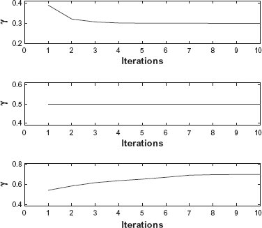
Estimates of normal contamination γ for iterations 1–10 of the EM algorithm and three simulated replicates with different values of γ: γ = 0.3 (top), γ = 0.5 (middle), and γ = 0.7 (bottom). The initial value for γ was 0.5 in all simulations.

These results can be compared to those from the simulation study by Lamy et al. ¹⁷ For a normal contamination of 30% the results are similar, but for 45%, which is the largest fraction studied by Lamy et al, their method provides 8%–18% incorrectly estimated probes while at 50% contamination our model provides an error rate below 1%. In addition, the present model performs well even at such a high amount of normal contamination as 70%, when the Markov state is correctly reconstructed at more than 97% of the probes. Obviously the differences between our results and those of Lamy et al depend not only on the different estimation algorithms but also on differences between the number and location of the probes, and on the model for the observed allele intensities and its parameters. However, given the magnitude of the performance improvement, a significant part of it must be attributed to the estimation algorithm as such.

4.2. Application to clinical data

We applied our method to a number of samples from the data described in Section 2. An example is displayed in Figure 3, which shows the Viterbi reconstruction of the Markov chain as well as the corresponding copy numbers compared to the data, for chromosome 3 in primary sample PD1753. For the Gamma priors for λ _c and η _c we chose shape parameters 2 and means 10^–15.

Figure 3.

Top: Viterbi reconstruction of the Markov path for chromosome 3 in PD1753. Bottom: sum of (standardized) allele intensities for probes within the same chromosome (grey dots), and the copy number of the corresponding state (black solid line).

The reconstruction divides the chromosome into two regions, reconstructed to state 2 ({A, B}) and state 4 ({AA, AB, BB}) respectively. As a simple check of this reconstruction we plotted the standardized allele intensities against each other for all probes in the respective region (Figs. 4–5). Figure 5, corresponding to the normal state, shows three clusters representing the three genotypes AA, AB and BB, while Figure 4 shows four clusters. In Table 1 state 2 is associated to two genotypes, A and B, but with normal contamination this state comprises four combined genotypes (1 + γ)A, AγB, γAB and (1 + γ)B (Table 2). Here γ is estimated at 0.53.

Figure 4.

Scatter plot of standardized measured allele intensities in the segment reconstructed to Markov state 2 in Figure 3. The fraction of normal contamination was estimated at 0.53.

Figure 5.

Scatter plot of standardized measured allele intensities in the segment reconstructed to Markov state 4 in Figure 3.

For some of the genomes the values of A_0kc, A_1kc B_0kc and B_1kc needed small adjustments before applying our model; without it, the model did not produce a reasonable fit. A possible explanation for this adjustment being required is a drift in the measured intensities from when data from the wild-type samples, used to estimate most model parameters, was collected, to when the tumor samples were analyzed. A suitable construction of the adjustment was as a common, ie, genome-wide multiplier c₀ for all A_0kc and B_0kc, and another common multiplier c₁ for all A_1kc and B_1kc. The multipliers c₀ and c₁ were estimated using data from a chromosome segment known to belong to the normal state. The data within this segment was clustered into three parts using the k-means algorithm, and then c₀ and c₁ were estimated by a least squares fit.

5. Discussion

We have presented a method to estimate the number of copies of each of the two alleles in SNP data, taking three features common in cancer data into account; unequally spaced probes, aneuploidy, and normal contamination. Unequally spaced probes are modeled using a continuous-index Markov chain instead of a discrete-index one, which is the usual choice in the literature. The ploidy and fraction of normal contamination are both included as parameters in the model, which allows us to estimate them along with other variables and using all the data, rather than estimating them separately in a pre-processing step. This set-up also allows us to retain the integer structure of the allele copy numbers. The model's ability to estimate the fraction of normal contamination has been demonstrated in a simulation study, with the results being far better than for previous methods and excellent even with as much as 70% normal contamination.

Above we denoted Markov state 4, ie, the state with genotypes {AA, AB, BB}, the normal state, irrespective of the ploidy of the chromosome. The reason for singling out this particular state is that it is often particularly interesting whether the Markov chain is in this state or not, at any given probe. One could argue that if the ploidy differs from two this is not ‘normal’, but it is straightforward to select a different state as ‘normal’ and then modify the transition rate structure and estimation algorithm accordingly.

The emission model, ie, Eqs. (1)–(4), assume that the means and variances of the measured intensities are both linear in the amount of each allele. In practice this assumption may fail, eg, because for large copy numbers the response is nonlinear. One could then include such a non-linearity in the model, and model the mean intensities as ${\mu }_{kcg}=h_{kc}\left(g;{\theta }_{kc}\right)$ where h is some function and θ _kc parameters of this function. Ideally the functional form h as well as all its probe-speficic parameters θ _kc should be well estimated beforehand, so that they are essientially known when evaluating an unknown sample. Similar comments apply to the variance of the measured intensities.

In this paper we have only considered probes that provide allele-specific intensity measurements, but, as mentioned in Section 2, microarrays often also contain probes that measure the total copy number only, ie, the sum of the number of alleles. Such probes can easily be included in our model by speficying a corresponding suitable emission density, ie, a density corresponding to Eq. (3). For instance, this could be a univariate Normal density with mean ${\mu }_{kcg}=C_{0kc}+C_{1kc}\left(g_{\text{A}}+g_{\text{B}}\right)$ and variance ${\sigma }_{kcg}^2=v_{kc}{\mu }_{kcg}^2$ for parameters C_0kc, C_1kc and v _kc that again need to be estimated prior to analyzing an unknown sample. Should the response function from total copy number to intensity not be linear for large copy numbers, this could be handled similarly to what can be done for SNP probes; cf. the previous paragraph.

Finally we mention some possible limitations of our method. Firstly, the accuracy of the method is likely to be reduced in regions of very high copy number where signal saturation occurs, such as in amplicons, and bespoke nonlinear adjustments may be required (as discused above). Secondly, we have ignored copy number polymorhisms. These will produce non-integer copy numbers in the cancer sample due to the skewed ratio between the cancer and the contaminating normal. If copy number data is available for the normal, it may be possible to generalise these methods to make such an adjustment, however, such regions are generally a lot smaller in scale than the somatic copy number changes seen in cancer and were not considered further. Lastly, we have assumed that the sample in question is derived from a homogeneous collection of cells. However, cell-to-cell variation is quite possibly going to produce a lot of different clones with differing copy numbers, and more general methods will be required to deal with such complexities.

To sum up this paper, copy number variations in cancer are common and their accurate determination is important for determining homozygous deletion, amplifications and breakpoints, all of which can be functionally implicated in cancer. This problem is compounded by normal contamination, making the accurate estimation of integer copy numbers in cancer samples with normal contamination difficult. Here we have introduced a method that addresses this problem.

Disclosure

This manuscript has been read and approved by all authors. This paper is unique and is not under consideration by any other publication and has not been published elsewhere. The authors and peer reviewers of this paper report no conflicts of interest. The authors confirm that they have permission to reproduce any copyrighted material.