Sage Journals: Discover world-class research

Abstract

We introduce a Chaste plugin for the generation and the simulation of Gene Regulatory Networks (GRNs) in multiscale models of multicellular systems. Chaste is a widely used and versatile computational framework for the multiscale modeling and simulation of multicellular biological systems. The plugin, named CoGNaC (Chaste and Gene Networks for Cancer), allows the linking of the regulatory dynamics to key properties of the cell cycle and of the differentiation process in populations of cells, which can subsequently be modeled using different spatial modeling scenarios. The approach of CoGNaC focuses on the emergent dynamical behavior of gene networks, in terms of gene activation patterns characterizing the different cellular phenotypes of real cells and, especially, on the overall robustness to perturbations and biological noise. The integration of this approach within Chaste's modular simulation framework provides a powerful tool to model multicellular systems, possibly allowing for the formulation of novel hypotheses on gene regulation, cell differentiation, and, in particular, cancer emergence and development. In order to demonstrate the usefulness of CoGNaC over a range of modeling paradigms, two example applications are presented. The first of these concerns the characterization of the gene activation patterns of human T-helper cells. The second example is a multiscale simulation of a simplified intestinal crypt, in which, given certain conditions, tumor cells can emerge and colonize the tissue.

Keywords

multiscale modeling gene regulatory networks cell differentiation attractors cancer development chaste

Introduction

To exploit the ever-increasing amount of biological data available, efficient mathematical and computational models are becoming essential instruments for both theoretical and experimental biologists.^{1, 2} Multicellular systems, such as tissues and organs, can be now qualitatively and quantitatively investigated via a large number of efficient modeling frameworks, which usually develop into useful simulation and analysis tools.³

Multiscale modeling approaches have proven reliable in representing complex biological phenomena at different abstraction levels, allowing one to capture processes with separate spatiotemporal scales, their hierarchies, and their communication rules.^{4, 5} In the case of tissues and organs, these include intracellular processes such as gene regulation, and intercellular processes such as molecular signaling via pathways and microenvironment interactions. Phenomena such as tissue patterning, cellular migration, homeostasis, and clonal dynamics emerge from this interplay that, when disrupted, can lead to tumorigenesis and cancer development.^{6, 7}

In this context, an effective and comprehensive multi-scale modeling framework is that provided by Chaste (Cancer, Heart and Soft Tissue Environment^{8, 9}), a general-purpose simulation tool aimed at the representation and the analysis of complex phenomena and processes in biology and physiology. Chaste divides into two main application areas: 1) cardiac Chaste, for continuum modeling of cardiac electrophysiology, and 2) cell-based Chaste, for individual-based modeling of cell populations. In particular, cell-based Chaste provides the modeler with multiple approaches to account for the spatial features of a system (via, eg, on- and off-lattice representations of the geometry) and allows him or her to define deterministic force laws between cells or stochastic update rules for cell–cell interactions, cell killer objects (eg, for apoptosis), cell-cycle models, and cell mutation states. In general, cell-based Chaste provides a computational framework bridging across spatial and temporal scales within a single modeling tool, thus allowing the user to define and run multiscale simulations (for a recent and exhaustive review on multiscale modeling frameworks for the simulation and analysis of multicellular systems, see Ref. 3).

In this paper, we introduce CoGNaC (Chaste and Gene Networks for Cancer), a Chaste plugin for the multiscale modeling of multicellular systems where gene regulatory interactions are accounted for explicitly. This tool links the dynamics of gene regulatory networks to key properties of cell cycle and differentiation processes, to drive the spatial evolution of multicellular systems in cell-based Chaste. The possibility of modeling multicellular systems in cell-based Chaste makes it possible to use CoGNaC in various spatial-modeling scenarios.¹⁰ We stress that the plugin is not tailored toward a specific tissue or organ, but it is meant to be completely generic. In this first version, CoGNaC adopts the approach of noisy random Boolean networks (NRBNs)^11–13 to model gene regulatory networks (GRNs). Other modeling approaches have been used to describe GRNs, reproduce experimental data, and provide novel predictions. These are often ascribed to the broad categories of deterministic, stochastic, or hybrid approaches, according to their quantitative representation of the network (see Refs 15,16 and references therein).

Grounded in statistical physics and complex systems science, NRBNs are an abstract model of gene regulation relating cell differentiation to the robustness of cells against biological noise and specific perturbations.¹³ This well-known approach focuses on the emergence of dynamical behavior by combining a Boolean representation of genes’ activity with a simplified form of regulatory interaction, the rationale being that no static analysis can capture the overall complexity gene regulation processes. When compared to other approaches (eg, deterministic or stochastic ones, for a review see Ref. 14), the Boolean abstraction allows for an effective and unambiguous characterization of the gene activation patterns that characterize distinct cellular (pheno)types. A key goal is to investigate the generic properties of GRNs, ie, those properties shared by a broad range of distinct networks, by means of massive statistical ensemble analyses of networks under certain biological constraints. (Even though the approach clearly relies on several abstractions, it was repeatedly proved fruitful to investigate key emergent properties of real networks.^17–22 Also, the simulation of the dynamics of completely characterized regulatory architectures and circuits with a Boolean representation is recently gaining great attention).^23–25

Therefore, on one hand, CoGNaC can be effective for computational and experimental biologists to analyze dynamical emergent properties of GRNs when their regulatory interactions are known, eg, available from public databases, hence allowing one to uncover relations and phenomena that a simple static analysis would probably fail to detect. On the other hand, by generating and simulating ensembles of networks sharing structural and functional parameters, CoGNaC allows one to investigate the generic properties of still partially characterized GRNs, possibly providing an ensemble-level understanding of experimental phenomena. A detailed description of the GRN model is provided in the next section.

Moreover, thanks to the fine integration with Chaste, CoGNaC delivers a comprehensive multiscale modeling and simulation framework in which the GRN dynamics drives key properties of the cell cycle, cell growth, and the differentiation fate of cells, thus linking the emergent properties of the GRN to the morphological dynamics of the tissue. Therefore, the use of CoGNaC with Chaste offers a powerful tool to model multicellular systems, possibly allowing the formulation of novel hypotheses on gene regulation and cellular differentiation. Furthermore, and more importantly, the explicit representation of GRNs might allow the qualitative and quantitative assessment of the role of genomic alterations, eg, somatic mutations, in the emergence of tumors, at both the network and tissue levels.

The remainder of this paper is structured as follows. In the next section, the GRN model based on NRBNs is described, and subsequently the spatial modeling framework provided by Chaste is introduced. In section “The multiscale link,” the link connecting the emergent dynamical properties of the GRNs to the physical properties of the model at the tissue level is explained. In the next section, the main features of CoGNaC are described. Then, two example applications of CoGNaC are discussed, one concerning the analysis of the gene activation patterns of human T-helper cells and the other regarding the simulation of a simplified model of cancer development in a multicellular structure resembling an intestinal crypt. We finally summarize the conclusions and indications on further works, and finally give in the Appendix some details concerning the implementation of CoGNaC.

Noisy Random Boolean Network Models of Gene Regulatory Networks

Classic random Boolean networks (RBNs) were introduced by Kauffman to represent regulatory networks.^{26, 27} An RBN is graph with n Boolean nodes associated with Boolean variables σ_i ∈ {0, 1}, representing the activation of a gene: if σ_i = 1, then the ith gene synthesizes its product (ie, proteins or RNAs). Each node is connected to k_i ≤ n – 1 input nodes implementing the regulatory function, ie, those genes that influence the activation of the ith gene. Thus, the value of the node σ_i at time t + 1 is determined according to a Boolean function f_i of the input nodes at time t.

The deterministic evolution of the system consists of a parallel update of all nodes, at any discrete time step, and moves over configurations of the values in all nodes (ie, states). Since classic RBNs are synchronous and deterministic, any dynamical trajectory will necessarily end up in a limit cycle, which is a finite, ordered sequence of configurations that endlessly repeat in time; this will be termed attractor, as in the jargon of dynamical systems (Fig. 1B). The biological interpretation is that all the cells of an organism share the same genome, yet each cellular function, eg, phenotype, is characterized by a specific dynamical gene activation pattern, in which some genes are always highly expressed (eg, housekeeping genes), others always inactive or oscillating with some particular scheme. Accordingly, in our approach all the cells share the same GRN, ie, the NRBN, whereas the attractors represent the distinct gene activation patterns.

Figure 1

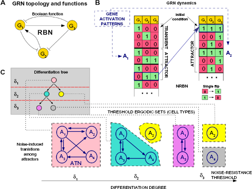
GRN model of cell differentiation in CoGNaC. Simplified representation of cell differentiation via NRBNs. (A) Example RBN with three genes (nodes) and edges subsuming regulatory interactions (via a Boolean function, not shown). (B) Example dynamics to highlight network's attractors, which model gene activation patterns A₁,…, A₅, and possible transitions among them induced by noise (ie, single flips). (C) These transitions yield an attractor transition network that generates five cellular types when three thresholds, δ_i, are evaluated and the corresponding threshold ergodic sets computed. In this model, where the efficiency of noise-control mechanisms are related to differentiation types, stem cells (pink), intermediate stages (light blue), and fully differentiated cells (yellow, purple and gray) emerge. The corresponding differentiation tree is shown (Fig. modified from Ref. 7).

Along the lines of Ref. 13, noise-resistance mechanisms of RBNs – and hence of GRNs – can be related to cellular differentiation processes yielding Noisy RBNs (NRBNs). By randomly changing node values in an attractor state (ie, single-node “flips”, such as switching a gene “off” or “on”) and recomputing the network dynamics, noise-induced transitions among the attractors can be detected (Fig. 1B). When this process is repeated in a systematic way, a stability matrix, also called the attractor transition network (ATN), determines how robust a gene activation pattern is to biological “noise” (the more frequently the network dynamics jumps to another attractor, the more unstable the attractor is) (Fig. 1C). On top of this complex machinery, since noise-control mechanisms are known to be related to the degree of differentiation,^28–32 NRBNs define a dynamical model of cell differentiation.

Consider an NRBN attractor A_i (ie, a limit cycle of the network dynamics standing for a specific gene activation pattern): another attractor A_j is “δ-reachable” from A_i if at least a fraction δ of different single-node flips (in any state of A_i) leads the dynamics to switch from A_i to A_j. A set of attractors such that 1) all the attractors in the set are mutually δ-reachable and 2) no attractors in the set are δ-reachable from any attractor not belonging to the set is defined as a threshold ergodic set (TES). The above conditions are equivalent to selection of strongly connected components, restricted to δ-reachability.¹³

By picking increasingly higher thresholds for δ, a hierarchical structure of such sets emerges from the original ATN (at δ = 0), and this allows us to characterize a specific degree of differentiation with a specific threshold. Thus, TESs represent cell types showing gene activation patterns varying as differentiation progresses. At δ = 0, one typically has a unique TES with many interconnected attractors, which represents less differentiated cells (eg, toti- and multi-potent stem cells). For higher δ, TESs break into disjoint smaller components (ie. intermediate stages) until fully differentiated cells have TESs with a unique stable gene activation pattern. This hierarchy among cell types identifies a specific differentiation tree, which emerges from the NRBN (Fig. 1C). This approach is general (ie, it is not related to a specific organism) and reproduces key phenomena of the differentiation processes, eg, hierarchical, stochastic, and deterministic differentiation strategies and induced pluripotency.³³

This is the model of cell differentiation implemented in CoGNaC, and represents the GRN component of the multi-scale framework. Emergent properties of this model are further linked to tissue-dynamics, as explained in a later section.

Representation of the Morphological Dynamics via Chaste

The wide range of modeling frameworks available within Chaste allow us to use the generic cell models provided by the CoGNaC plugin in a variety of cell-based settings. In particular, several distinct modeling approaches for the representation of the spatial dynamics of cell populations in tissues and organs are provided by the cell-based component of Chaste, namely 1) lattice-free models, such as center-based models, in which the connectivity is defined by Voronoi tessellations,^{34, 35} and vertex-based models,³⁶ and 2) lattice-based models, such as the cellular Potts model (CPM)³⁷ and other cellular automata (CA) models.³⁸ In general, lattice-free approaches aim at modeling the geometry and the physics of the system in a realistic way, yet, as they involve biomechanical forces and complex geometries, the space of parameters and variables can be dramatically large. Conversely, lattice-based models use simplified cellular automata-based representations of multicellular systems to describe cell displacement, movement, and interactions. Clearly, the optimal tradeoff between the complexity of the model and that of the represented phenomena and processes depends on the research focus.

In the following, we briefly outline the main features of the center-based Voronoi tesselation model, which is successively used in one of the two example applications. For a description of the other spatial models implemented in Chaste, see Ref. 9, whereas for an exhaustive comparison of the spatial modeling approaches for multicellular systems see Ref. 3.

Center-Based Spatial Model

The center-based Voronoi tessellation model included in the Chaste cell-based component is an off-lattice model, developed by Meineke et al.³⁵ and subsequently used by van Leeuwen et al.³⁹ as a model of intestinal crypt dynamics. Each cell is connected to neighboring cells by linear springs, where the cell neighbor is determined by a Delaunay triangulation and the cell shape is determined by the dual of the triangulation, the Voronoi tessellation.

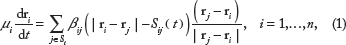
Specifically, inertial effects are neglected, and the viscous drag on cell centers is balanced with cell–cell interaction forces associated with the compression and extension of the springs connected to the neighboring cell centers. Accordingly, the equations of motion are

μ_{i} \frac{d r_{i}}{d t} = \sum_{j \in S_{i}} β_{i j} (| r_{i} - r_{j} | - S_{i j} (t)) \frac{(r_{j} - r_{i})}{| r_{j} - r_{i} |}, i = 1, \dots, n,

(1)

where t is time, r_i is the position of cell center i, n is the overall number of cells, S_ij(t) and β_ij are the rest length and the elastic constant, respectively, of the spring connecting cell centers i and j, S_i is the set of cells that are adjacent to cell i, μ_i is the drag coefficient, which depends on cell i's type and models the cell–stroma adhesion.

In the current implementation, when cell i divides after a full cell cycle (characterized by a specific duration), its daughter cell j is positioned at a distance of 0.1 cell diameters from cell i, in a randomly chosen direction. In order to model cell growth, the rest length of the spring connecting parent and daughter cell, S_ij(t), increases from 0.1 to 1 (natural length) in a time span equal to ϕ (default = 1 hour) (for more details see Ref. 40).

The Multiscale Link

Low-level properties emerging from the internal GRN can drive high-level physical properties of the model at the tissue level.⁷ This approach is independent from Chaste's framework chosen for spatial representation of the tissue (center-based, vertex-based, CPM or CA).

Recall that all the cells share the same genome – thus the same GRN – yet every single cell is characterized by a specific degree of differentiation and a specific type as time progresses. From a modeling perspective, in CoGNaC, a unique NRBN is computed, and each cell is allowed to track – in its “internal” state - the gene activation pattern that is driving its dynamics, eventually jumping among attractors while differentiating. Accordingly, emerging properties of the NRBN drive cell-type-specific cellular properties such as 1) cell cycle length and 2) differentiation fate at the spatial level (Fig. 2).

Figure 2

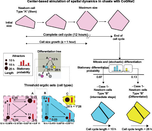
Multiscale link in CoGNaC. The dynamics of NRBNs at the GRN level drives key properties of the cells in the spatial model, which, in this example, is based on the center-based model implemented in Chaste and described in section “Representation of the morphological dynamics via Chaste”. Assume that the selected NRBN predicts the bottom-left threshold ergodic sets – we use those to link cell cycle length and differentiation fate to the spatial evolution of the cells. In the example, a newborn stem cell requires 12 hours to end its cell cycle and divide, as computed from the average of the lengths (here measured in hours) of the four attractors belonging to the TES “A” (pink), weighted on the stationary probabilities. The cell reaches its maximum size after ~1 hour, which is the time needed for the spring of a newborn cell to reach its natural length, ie, φ; = 1 hour. When dividing, the differentiation fate (either type “B”, light bvlue, or “C”, yellow, for both the daughter cells) is probabilistically determined on the basis of the stationary probability of the patterns in TESs “B” and “C” (Fig. modified from Ref. 7).

Cell Cycle Length

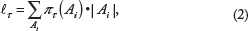
Recall that a cellular type is mapped to a TES, which is a collection of interconnected gene activation patterns, given a specific resistance to noise. It is natural to expect that some of those patterns will be prevalent, so cells of that type, before differentiating, will tend to express a subset of such patterns. The ergodicity property of TESs makes it natural to think of such patterns as a particular type of stochastic process that possess a stationary probability π – the probability of observing a specific pattern expressed, in the long run. (This is derived mathematically by interpreting an ATN as a discrete-time Markov chain and applying standard numerical techniques to estimate π.)

So, patterns with higher stationary probability would be more relevant. In general, one would like to link an emergent property such as the cell cycle length for a cell of type τ, to the “length” of such attractors proportionally weighted with their long-run probability.

Putting this formally, if π_τ(A) is the stationary probability of attractor A in the TES modeling cell type τ, the length ℓ_τ of the cell cycle for a cell of that type is

ℓ_{τ} = \sum_{A_{i}} π_{τ} (A_{i}) \cdot | A_{i} |,

(2)

where |A_i| is the pattern length (number of different configurations it contains).

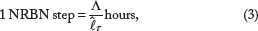
A conversion between the time-units of the GRN dynamics (ie, the NRBN step, an abstract time unit) and that of the spatial model (hours, in Chaste) is then required. Following Ref. 7, we link the internal and external timescales as

1 NRBN step = \frac{Λ}{{\hat{ℓ}}_{τ}} hours,

(3)

where

{\hat{ℓ}}_{τ}

is the average of the cell cycle values predicted by Equation (2) and ∧ is the analogous cell-cycle time at the spatial level (in hours). Hence, the relative difference in the lengths of the cell cycles of the cells of different types accounts for the difference in the replication paces, and emerges from the GRN model. Notice that this link can be set regardless the modeling approach chosen to represent a tissue in Chaste.

Differentiation Fate

Following Ref. 13, it is possible to hypothesize that cells wander across gene activation patterns that are specific to their own cell type, according to random genomic mutations that can be estimated from experimental data.⁴¹ In our theoretical framework, it is possible to (probabilistically) estimate in which pattern (ie, attractor) the cell will be found when reaching the mitosis stage, on the basis of the distinct stationary probabilities of the attractors belonging to a TES. Once chosen, the cell type of the daughter cells will be given by the TES (with successive increasing threshold) in which the selected attractor is included, thus describing the process of stochastic differentiation (Fig. 2).

Main Features of CoGNaC

CoGNaC can generate and simulate a random NRBN model with some predefined structural features, or a specific hard-coded network model may be specified.

Network Modeling

Three distinct modes for the generation of NRBNs are available:

Random Generation

CoGNaC can create random networks with the following structural parameters: 1) number of nodes N; 2) average network connectivity K (average number of edges for each node); 3) network topology (either Erdos-Renyii,¹² or Barabasi–Albert's preferential attachment scale-free⁴²); 4) probability p of associating a canalyzing function to a random node (whereas, 1 – p is the probability of associating a random Boolean function).²⁰ (The distribution of regulatory rules is likely to be structured and not completely random. A canalyzing function has at least one input such that if that input is set then the output value is fixed. In GRNs, this is analogous to saying that some genes are mainly regulated by one other gene.)

Custom Structure, Random Regulatory Interactions

An NRBN structure can be provided via a file in the Graph Modeling Language syntax (gml file); CoGNaC can then associate Boolean functions to the nodes, with the previously defined parameter p.

Custom Structure and Regulatory Interactions

A complete description of a network and its Boolean regulatory interactions can be passed to CoGNaC through standard network definition files, such as, eg, net and cnet files.⁴³

Network Simulation

CoGNaC can process any randomly generated or inputted network. The tool searches for the limit cycles (ie, the NRBN attractors, standing for gene activation patterns) by performing an exhaustive search (see the Appendix for the algorithmic details). The number of configurations of each attractor will be successively used in the multiscale model, to define the cell cycle length of cell types at the spatial level (see section “The multiscale link”).

Afterward, the stability to noise of each attractor is tested, by performing one-time-step single-flip (ie, 1 → 0 or 0 → 1) perturbations of random nodes in random positions in the attractors. The noise-induced probability of switching between attractors defines the ATN; an automatic algorithm for thresholds detection and TES estimation allows the extraction of a hierarchical differentiation tree. In turn, stationary probabilities are computed to complete the multiscale link (see section “Noisy Random Boolean Network Models of Gene Regulatory Networks”).

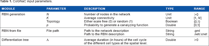
When CoGNaC is asked to generate a random network, the process can be iterated until a user-specified differentiation tree is matched by the generated network. This allows one to constrain the generation of GRN models so that the emergent differentiation patterns fits the provided biological data. Once a suitable NRBN is found, time-unit conversion concludes this phase. We refer to Table 1 for the definition of the main CoGNaC parameters.

Table 1

CoGNaC input parameters.

MODULE	PARAMETER	DESCRIPTION	TYPE	RANGE
RBN generation	N	Number of nodes in the network	Unit	>0
	K	Average connectivity	Unit	[1, N]
	Topology	Either scale free (0) or random (1)	Boolean	{0,1}
	p	Probability to generate a canalyzing function	Double	[0,1]
RBN from file	File path	Path to the network description	String	.gml
		Path to the RBN description	String	.net/.cnet
Differentiation tree	Λ	Average duration (in hours) of the cell cycle of the different cell types at the spatial level.	Double	>0

Example Applications

The CoGNaC plugin may be used generically within Chaste across a variety of modeling scenarios. We here present two applications of CoGNaC: the first in which the gene activation patterns of a real GRN, specifically that of human T-helper cells, are determined and investigated, confirming current evidence from experimental publications; the second regarding a simplified intestinal crypt-like multiscale model where, in certain cases, tumor cells emerge and start colonizing the tissue.

Gene Activation Patterns in T-Helper Cell Differentiation

Dynamical modeling and simulation of real architectures of GRNs is increasingly gaining attention, mostly in conjunction with the characterization of gene activation patterns identifying specific cellular functions, which are often not explainable with static analysis of genes and their interactions. Despite the underlying abstractions, Boolean modeling appears to be effective to this end and can be exploited with CoGNaC. In this example, the signaling network that drives the differentiation of T-helper (Th) cells – which is structurally and functionally characterized⁴⁴ – was analyzed with CoGNaC (Fig. 3). Note that several studies showed that this network is sufficient to qualitatively describe the real differentiation process of Th cells, see, eg, Ref. 45.

Figure 3

T-helper signaling network analysis. (Upper left) The regulatory network that rules the differentiation process of Th cells. Positive regulatory interactions are shown with green arrows, and negative interactions with red ones.⁴⁴ (Bottom) The three single-point attractors of the T-helper network detected by CoGNaC are shown. On the column header, the names of the genes are displayed, from Ref. 45. Each row corresponds to a specific attractor of the network, which is denoted by the corresponding cell type, namely Th0, Th1, and Th2. In the table, black cells represent inactive genes and white cells active genes. (Upper right) The stability of the gene activation patterns in terms of attractor transition network. Each edge stands for the probability of switching from a specific gene activation pattern (Th0, Th1, or Th2) to another, as a consequence of a random single-gene flip.

In brief, the human immune system includes several cell populations, including antigen-presenting cells, natural killer cells, and B and T lymphocytes. T lymphocytes can be divided into Th cells and T-cytotoxic cells (Tc). Th cells participate in cell- and antibody-mediated immune responses by secreting various cytokines, and they are subdivided into different cell types depending on the set of cytokines that they secrete.⁴⁶

In Figure 3 we show the three single-point attractors detected by CoGNaC on the Th network, as well as their stability in terms of ATN. It should be noted that these attractors indeed represent the gene activation patterns of the three main phenotypes characterizing the unperturbed T-helper network, namely, Th0, Th1, and Th2 cells. From experimental evidence (see, eg, Ref. 44), in fact, Th0 cells are supposed to produce none of the cytokines included in the model, ie, (IFN-β, IFN-γ, IL-10, IL-12, IL-18, and IL-4). The gene activation pattern representing Th1 cells, instead, is characterized by high activation of IFN-γ, IFN-γ R, T-bet, and SOCS1. Finally, in Th2 cells high level of activation of GATA-3, IL-10, IL-10R, IL-4, IL-4R, STAT3, and STAT6 are observed.

Besides, by simply assessing the patterns’ stability, it is possible to hypothesize that Th0 type is the less resistant to biological noise and specific perturbations (eg, triggering signals) and, thus, it might represent an unstable precursor stage in a differentiation path toward the more stable Th1 and Th2 types. This hypothesis is experimentally validated, as the Th cells’ differentiation process is supposed to proceed from precursors Th0 toward the effectors Th1 (secreting IFN-γ) and Th2 (secreting IL-4), which also appear to be more stable against perturbations.⁴⁶

We remark that this example serves as a proof of concept to show the usefulness and accuracy of CoGNaC in assessing the gene activation patterns of real gene regulatory networks and their stability. A direct application to more complex networks and biological phenomena will be achievable once experimental data on real architectures and regulatory functions becomes available, especially in regard with the investigation of the so-called cancer attractors (see, eg, Refs 47,48).

Cancer Cell Colonization of a Colon Crypt

A simplified multiscale model of a multicellular system that structurally resembles an intestinal crypt was designed and simulated with CoGNaC and Chaste. The model combines a center-based 2-D representation of cells at the spatial level, and an NRBN-based underlying GRN, as described in section “Noisy random Boolean network models of gene regulatory networks”.

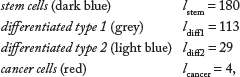
In particular, a certain number of structurally analogous NRBNs have been generated with the following parameters: 100 nodes, Alberts–Barabasi's preferential attachment scale-free topology, average connectivity K = 3, and mixed Boolean functions. These parameters were chosen, in accordance with similar studies,^{7, 49} as the number of nodes is in agreement with the number of estimated driver genes in colorectal cancer⁵⁰ and the topology is supposed to be plausible for real GRNs.^{51, 52} Among all the simulated networks, a specific one was then selected because of the properties of the emerging differentiation tree and of the attractor landscape (see Fig. 4 for details): the differentiation tree predicted by CoGNaC includes four cell types: a stem-like cell type (TES with δ = 0) and three differentiated cell types (three distinct TESs at δ = 0.45). Note that one of these non-stem types is characterized by a very low stationary probability and a short cycle length, thus reasonably representing cancer cells – unlikely to emerge, but with very fast proliferation pace. This network was specifically selected to allow the investigation of the scenarios under which the GRN dynamics may lead to cancer cells colonizing a healthy crypt.

Figure 4

GRN model in the example crypt simulation. (Upper left) The NRBN generated by CoGNaC has 100 genes, is scale-free, and each regulatory interaction depends, on average, from K = 3 other genes. Oriented edges represent regulation paths, the size of each node being proportional to its network degree and each color corresponding to the type of regulatory interaction (see the legend in the figure). (Upper right) Three different gene activation patterns are predicted (landscape of attractors where each node is a NRBN configuration). (Lower left) Noise-induced transition probabilities among attractors and their stationary probabilities. (Lower right) The emerging differentiation tree is displayed. The root of the tree is the TES including all attractors (resembling stem cells), and determines a cell cycle length as the average length of the three attractors, weighted by their stationary probabilities. The leaves of the tree correspond to two differentiated cell types plus a cancer type that is characterized by a short cell cycle length and a very low likelihood of occurrence. Visualizations were performed with the CABERNET tool.⁶⁰

Predicted cell types have the following cell cycle lengths, in NRBN time steps:

stem cells (dark blue)	l_stem = 180
differentiated type 1 (grey)	l_diff1 = 113
differentiated type 2 (light blue)	l_diff2 = 29
cancer cells (red)	l_cancer = 4,

their stationary probabilities being π _stem = 1, π _diff1 ⋍ 0.94, π _diff2 ⋍ 0.05 and π_cancer ⋍ 0.002.

The Chaste tissue is built by displaying 20 × 20 = 400 hexagonal stem cells at time t = 0 on a 2-D rectangular space with left-hand, right-hand, and bottom closed boundaries (ie, cell centers cannot move through these boundaries), whereas the upper side is left open, allowing cells to be expelled due to mitotic pressure. The parameters of the spatial model were chosen in line with⁵³ and, in general, the whole morphological representation of the crypt is meant to be a simplified version of that proposed in Ref. 7, specifically aimed at the investigation of cancer emergence in multicellular systems. Cells grow and divide according to a cell cycle length that is specific for the cell type (see section “The multiscale link” and Fig. 2). Given that the average cell cycle length is fixed to ∧ = 16 hours, in accordance with experimental data on intestinal crypt cell types,⁵⁴ and that ${\hat{ℓ}}_{r} = 63.5$ , we obtain the following relation

1 N R B N s t e p \approx 0.25 h o u r s

yielding the following cell-cycle timings: 27.2 hours for stem cells, 28.5 and 7.3 for differentiated type 1 and 2 cells, and 1 hour for cancer cells. In the initial configuration of the tissue, the age of stem cells is uniformly distributed in the interval [0: 27] hours. When stem cells asymmetrically divide (one daughter keeps the stem type), the differentiation fate is probabilistically chosen according to stationary probability of the differentiated TESs, whereas differentiated and cancer cells give origin to two daughter cells of the same type. Thus, we can expect a cancer cell to emerge – on average – after 500 stem cell divisions. In Figure 4 we summarize these findings.

One-hundred and forty independent stochastic simulations of crypt dynamics were performed, starting from equivalent initial configurations and lasting 1000 minutes (simulation time). Three behaviors were typically observed: (i) tissue homeostasis, (ii) control of cancer expansion via mitotic pressure, and (iii) cancer colonization; examples of these scenarios are displayed in Figure 5, along with further statistical analyses.

Figure 5

Crypt simulation scenarios: homeostasis, mitotic pressure, control and cancer colonization. (Top panels) Screenshots of the example multiscale simulations described in the text (further parameters of the spatial simulation are (a) spring stiffness, β = 30³⁵; growth duration, φ; = 0, ie, the time needed for the spring rest length of the newborn cells to increase up to the natural length; drag coefficient μ = 1 for any cell type). Three scenarios are shown. (i) Homeostasis, (ii) mitotic pressure control, and (iii) cancer colonization. Initially 400 stem cells are displayed in the crypt. After a transient time, differentiated cells appear due to mitotic events; some cells start being expelled from the upper open boundary. In scenario (i) at t = 1000 minutes, a reasonable balance between the different cell types is preserved. In scenario (ii), with the same initial conditions, a single cancer cell (red) emerges at t = 60 (not shown), but the resulting colony does not succeed in invading the tissue, because cancer cells are progressively pushed out of the tissue due to the mitotic pressure. Finally in scenario (iii), a cancer cell emerges at t = 500. This cell starts duplicating at a pace faster than other cell types (ie, as of a cell cycle length of about 1 hour, in spite of an average of 16 hours). Therefore, a spheroid-like dynamical structure involving an increasing number of cancer cell emerges and starts colonizing the system, pushing a progressively larger number of normal cells out of the crypt. (Bottom panels) The variation of cell populations in time is shown with respect to the three example simulation. Notice the rounds of progressive clonal expansions of cancer cells in the third scenario.

In the upper panel of Figure 5, a typical homeostatic behavior is shown [Scenario (i)], in which the proportion of stem and differentiated cells tends toward a dynamical equilibrium and no cancer cells originate, as quantified by the variation of cellular populations in time. Conversely in some cases, a cancer cell emerges and begins to proliferate, as it happens after 60 minutes in the simulation displayed in the middle panel of Figure 5. When this happens, the likelihood of cancer colonization strongly depends on the overall spatial arrangement, being less likely when cancer cells are close to the upper (open) boundary of the crypt. In this particular simulation, for instance, the number of cancer cells remains quite stable due to mitotic pressure [Scenario (ii)]. Furthermore, as it is observed in a certain number of simulations (see below), it is reasonable to expect that such cancer cells will be eventually expelled from the crypt, leading to a complete tumor eradication. In other words, the rapid turnover of intestinal crypts might act as a defense mechanism ensuring, sometimes, the maintenance of homeostasis by mitotic pressure, as cancer cells are expelled despite their fast replication pace. In some other cases, however, the outcome of these dynamics might be the opposite, as cancer cells indeed colonize the tissue and an increasingly larger number of differentiated cells are expelled out of the crypt. In that case, the fast-replicating cancer colony would tend to cluster in a spheroid resembling the early stages of a colorectal adenoma, as shown in the bottom panel of Figure 5 [Scenario (iii)].

In Figure 6, we quantitatively assess these observations by plotting the average density of cancer cells over time. One can notice that in some simulations, such a density reaches around 90% (complete colonization of the tissue), whereas in other simulations, the colonization fails, either because no cancer cells emerge or because of the mitotic pressure control. Summarizing these findings, homeostasis with no cancer cells is observed in 102 simulations of 140 (ie, around 73%) [Scenario (i)]; in 38 simulations (27%) at least one cancer cell originates, and this leads to a colonization in 27 cases (19%) [Scenario (iii)]; whereas in 11 cases (8%) mitotic control prevents the colonization [simulations in which less than 10 cancer cells are present were grouped in this category, Scenario (ii)]. We remark that the complete eradication of the tumor was observed in only three simulations of the latter cases. In the last panel of Figure 6, the probability distribution of cancer cell densities, computed in the simulations in which at least one cancer cell emerges, is shown (as a heatmap), highlighting the progressive appearance of very aggressive cancer colonies.

Figure 6

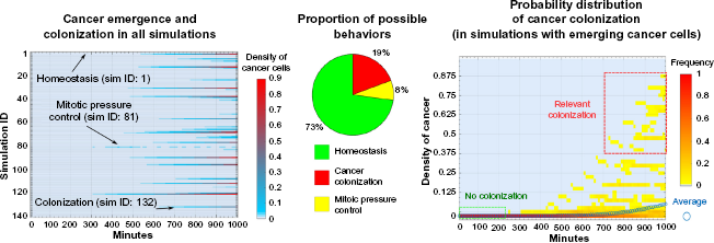
Statistical analysis of the crypt simulations. The statistical analysis of 140 independent simulations with identical initial configuration of the crypt (including the three examples of Fig. 5) is shown. In the left panel, the variation of the density of cancer cells (ie, the ratio of cancer cells over the total number of cells) in time with respect to all the simulations is shown. Notice that densities are computed on intervals of 10 minutes, and that very low densities (ie, <0.005) are not displayed in the graph. In the middle panel, the proportion of different behaviors observed in the simulations is displayed: (i) homeostasis: no cancer cells appear during the simulations; (ii) mitotic pressure control: at least one cancer cell emerges during the simulation, but at the end of the simulations there are fewer than 10 cancer cells; (iii) cancer colonization: more than 10 cancer cells are present at the end of the simulation. In the right panel, the probability distribution of the density of cancer cells, and the average value, computed only on simulations of scenarios (ii) and (iii) is displayed.

Notice that in Ref. 40 similar results are obtained in a center-based model of intestinal crypt (via Chaste), by modifying the drag coefficient μ (Equation 1) of a small set of mutant cells in an initially healthy crypt. The underlying rationale is that mutant cells showing an alteration of the Wnt pathway are characterized by a stronger cell–stroma adhesion (ie, increased drag) with respect to normal cells. Hence, given that mutant cells are more likely to persist in the crypt because of the greater resistance to the mitotic pressure, a colonization of the crypt may follow. Conversely, in our approach μ in normal and cancer cells is identical, and the crypt colonization is mainly due to the difference in the replication paces, thus hinting at the complementary relevance of both these biological phenomena in cancer development.

Conclusions and Future Work

The goal of this article was to introduce and describe CoGNaC, a Chaste plugin for the multiscale modeling and simulation of multicellular systems, that uses a GRN-based dynamical model of cell differentiation, and to show some of its potential applications.

In the two selected examples, we showed some of the utilities of CoGNaC within the modular Chaste library. CoGNaC can provide a fine instrument to investigate the complex interplay characterizing the behavior of multicellular systems, with particular focus on the possible emergence of dysfunctional dynamical structures such as tumors. For instance, CoGNaC was used in a multiscale simulation of a simplified intestinal crypt to assess the influence of emergent gene activation patterns on the homeostasis of the tissue. Interestingly, in certain cases, the activation of particular, and usually, unlikely patterns, due to random gene perturbations, was observed to lead to the emergence of fast replicating clones that quickly colonized the tissue, yielding spheroid-like structures resembling the first stages of colorectal adenomas. CoGNaC was also applied to experimental data on real GRNs, allowing, for instance, the formulation of hypotheses on the relation between genotype and phenotype and on the complex differentiation process of T-helper cells.

Many important refinements and developments of CoGNaC are under way, especially related to different GRN modeling approaches, which could be more suitable and effective when detailed quantitative data on real architectures will become available. To this end, for example, reliable and comprehensive models of tumor progression (see, eg, Ref. 55,56) could be sensibly integrated in the GRN model, in order to investigate the complex phenomenon of tumor origin and development with a multiscale framework.

Availability

Instructions on obtaining and using the code used in the paper are available at https://chaste.cs.ox.ac.uk/trac/wiki/PaperTutorials/CoGNaC. Instructions for installing and building Chaste are available from the same location. The tutorials included in this package will reproduce both the example applications discussed in the paper.

Author Contributions

Conceived and designed the experiments: SR, AG, GC. Analyzed the data: SR, AG, GC. Wrote the first draft of the manuscript: AG, GC. Contributed to the writing of the manuscript: SR, AG, GC, GM, JO, JPF, MA. Agree with manuscript results and conclusions: SR, AG, GC, GM, JO, JPF, MA. Jointly developed the structure and arguments for the paper: SR, AG, GC, GM, JO, JPF, MA. Made critical revisions and approved final version: SR, AG, GC, GM, JO, JPF, MA. All authors reviewed and approved of the final manuscript.

Footnotes

Appendix

References

Kitano

Computational systems biology.

Nature. 2002; 420(6912): 206–10.

Kaneko

Life: An Introduction to Complex Systems Biology. Springer-Verlag, Berlin, New York; 2006.

De Matteis

, Graudenzi

, Antoniotti

A review of spatial computational models for multi-cellular systems, with regard to intestinal crypts and colorectal cancer development.

J Math Biol. 2013; 66(7): 1409–62.

Noble

Modeling the heart – from genes to cells to the whole organ.

Science. 2002; 295: 1678–82.

Southern

, Pitt-Francis

, Whiteley

. Multi-scale computational modelling in biology and physiology. Prog Biophys Mol Biol. 2008; 96(1-3): 60–89.

Wong

S.Y.

, Chiam

K-H

, Lim

C.T.

, Matsudaira

Computational model of cell positioning: directed and collective migration in the intestinal crypt epithelium.

J R Soc Interface. 2010; 7: 351–63.

Graudenzi

, Caravagna

, De Matteis

, Antoniotti

Investigating the relation between stochastic differentiation, homeostasis and clonal expansion in intestinal crypts via multiscale modeling.

PLoS One. 2014; 5(9): e97272.

Pitt-Francis

, Pathmanathan

, Bernabeu

M.O.

. Chaste: a test-driven approach to software development for biological modelling. Comput Phys Commun. 2009; 180(12): 2452–71.

Mirams

G.R.

, Arthurs

C.J.

, Bernabeu

M.O.

. Chaste: an open source c++ library for computational physiology and biology. PLoS Comput Biol. 2013; 9(3): 1002970.

10.

Rubinacci

Noisy Random Boolean Networks Dynamics for Cellular Differentiation Using Chaste Environment [Master's thesis]. Milano: Department of Informatics, Systems and Communication, University of Milan-Bicocca; 2015.

11.

Ribeiro

A.S.

, Kauffman

S.A.

Noisy attractors and ergodic sets in models of gene regulatory networks.

J Theor Biol. 2007; 247: 743–55.

12.

Serra

, Villani

, Barbieri

, Kauffman

S.A.

, Colacci

On the dynamics of random Boolean networks subject to noise: attractors, ergodic sets and cell types.

J Theor Biol. 2010; 265: 185–93.

13.

Villani

, Barbieri

, Serra

A dynamical model of genetic networks for cell differentiation.

PLoS One. 2011; 6(3): 17703.

14.

Karlebach

, Shamir

Modelling and analysis of gene regulatory networks.

Nat Rev Mol Cell Biol. 2008; 9(10): 770–80.

15.

De Jong

Modeling and simulation of genetic regulatory systems: a literature review.

J Comput Biol. 2002; 9(1): 67–103.

16.

Heckera

, Lambeck

, Toepfer

, van Someren

, Guthke

Gene regulatory network inference: data integration in dynamic models – a review.

Biosystems. 2009; 96: 86–103.

17.

Kauffman

S.A.

At Home in the Universe. Oxford University Press, New York; 1995.

18.

Kauffman

S.A.

, Peterson

, Samuelsson

, Troein

Random Boolean network models and the yeast transcriptional network.

Proc Natl Acad Sci U S A. 2003; 100: 14796–9.

19.

Serra

, Villani

, Semeria

Genetic network models and statistical properties of gene expression data in knock-out experiments.

J Theor Biol. 2004; 227: 149–57.

20.

Kauffman

S.A.

, Peterson

, Samuelsson

, Troein

Genetic networks with canalyzing Boolean rules are always stable.

Proc Natl Acad Sci U S A. 2004; 101: 17102–7.

21.

Ramo

, Kesseli

, Yli-Harja

Perturbation avalanches and criticality in gene regulatory networks.

J Theor Biol. 2006; 242: 164–70.

22.

Serra

, Villani

, Graudenzi

, Kauffman

S.A.

Why a simple model of genetic regulatory networks describes the distribution of avalanches in gene expression data.

J Theor Biol. 2007; 249: 449–60.

23.

Sanchez

, van Helden

, Thieffry

Establishement of the dorso-ventral pattern during embryonic development of drosophila melanogasater: a logical analysis.

J Theor Biol. 1997; 189: 377–89.

24.

Sanchez

, Thieffry

A logical analysis of the drosophila gap-gene system.

J Theor Biol. 2001; 211: 115–41.

25.

Albert

, Othmer

H.G.

The topology of the regulatory interactions predicts the expression pattern of the segment polarity genes in drosophila melanogaster.

J Theor Biol. 2003; 223: 1–18.

26.

Kauffman

S.A.

Metabolic stability and epigenesis in randomly constructed genetic nets.

J Theor Biol. 1969; 22: 437–67.

27.

Kauffman

S.A.

Homeostasis and differentiation in random genetic control networks.

Nature. 1969; 224: 177.

28.

Hoffman

, Chang

H.H.

, Huang

, Ingber

D.E.

, Loeffler

, Galle

Noise driven stem cell and progenitor population dynamics.

PLoS One. 2008; 3(8): 2922.

29.

Lestas

, Paulsson

, Vinnicombe

Noise in gene regulatory networks.

IEEE Trans Automat Contr. 2008; 53: 189–200.

30.

Hayashi

, Lopes

S.M.

, Surani

M.A.

Dynamic equilibrium and heterogeneity of mouse pluripotent stem cells with distinct functional and epigenetic states.

Cell Stem Cell. 2008; 3: 391–440.

31.

Furusawa

, Kaneko

Chaotic expression dynamics implies pluripotency: when theory and experiment meet.

Biol Direct. 2009; 4: 17.

32.

Eldar

, Elowitz

M.B.

Functional roles for noise in genetic circuits.

Nature. 2010; 467: 167–73.

33.

Yamanaka

Elite and stochastic models for induced pluripotent stem cell generation.

Nature. 2009; 460: 49–52.

34.

Sulsky

, Childress

, Percus

J.K.

A model of cell sorting.

J Theor Biol. 1984; 106(3): 275–301.

35.

Meineke

F.A.

, Potten

C.S.

, Loeffler

Cell migration and organization in the intestinal crypt using a lattice-free model.

Cell Prolif. 2001; 34(4): 253–66.

36.

Nagai

, Honda

A dynamic cell model for the formation of epithelial tissues.

Philos Mag B. 2001; 81(7): 699–719.

37.

Graner

, Glazier

J.A.

Simulation of biological cell sorting using a two-dimensional extended potts model.

Phys Rev Lett. 1992; 69: 2013–7

38.

Figueredo

G.P.

, Joshi

T.V.

, Osborne

J.M.

, Byrne

H.M.

, Owen

M.R.

On-lattice agent-based simulation of populations of cells within the open-source chaste framework.

Interface Focus. 2013; 3(2): 20120081.

39.

van Leeuwen

I.M.M.

, Byrne

H.M.

, Jensen

O.E.

, King

J.R.

Crypt dynamics and colorectal cancer: advances in mathematical modelling.

Cell Prolif. 2006; 39(3): 157–81.

40.

Osborne

, Walter

, Kershaw

. A hybrid approach to multi-scale modelling of cancer. Philos Trans A Math Phys Eng Sci. 2010; 368(1930): 5013–28.

41.

Nachman

M.W.

, Crowell

S.L.

Estimate of the mutation rate per nucleotide in humans.

Genetics. 2000; 156(1): 297–304.

42.

Barabasi

, Albert

Emergence of scaling in random networks.

Science. 1999; 286: 509–12.

43.

Dubrova

, Teslenko

, Martinelli

Kauffman networks: analysis and applications.

Proceedings of International Conference on Computer-Aided Design (ICCAD'2005). IEEE and San Jose, CA, USA; 2005: 479–84.

44.

Mendoza

, Xenarios

A method for the generation of standardized qualitative dynamical systems of regulatory networks.

Theor Biol Med Model. 2006; 3: 13.

45.

Garg

, Di Cara

, Xenarios

, Mendoza

, De Micheli

Synchronous versus asynchronous modeling of gene regulatory networks.

Bioinformatics. 2008; 24(17): 1917–25.

46.

Murphy

K.M.

, Reiner

S.L.

The lineage decisions of helper t cells.

Nat Rev Immunol. 2002; 2(12): 933–44.

47.

Huang

, Ernberg

, Kauffman

Cancer attractors: a systems view of tumors from a gene network dynamics and developmental perspective.

Seminars in Cell & Developmental Biology. Elsevier, Amsterdam; 2009; 20: 869–76.

48.

Huang

, Kauffman

How to escape the cancer attractor: rationale and limitations of multi-target drugs.

Seminars in Cancer Biology. Elsevier, Amsterdam; 2013; 23: 270–8.

49.

Serra

, Villani

, Graudenzi

, Colacci

, Kauffman

S.A.

The simulation of gene knock-out in scale-free random Boolean models of genetic networks.

Netw Heterog Media. 2008; 3(2): 333.

50.

Tamborero

, Gonzalez-Perez

, Perez-Llamas

. Comprehensive identification of mutational cancer driver genes across 12 tumor types. Sci Rep. 2013; 3: 2650.

51.

Barabasi

Linked: The New Science of Networks. Perseus Publishing, New York; 2002.

52.

Barabasi

, Oltvai

Z.N.

Network biology: understanding the cell's functional organization.

Nat Rev Genet. 2004; 5: 101–13.

53.

Van Leeuwen

I.M.

, Mirams

, Walter

. An integrative computational model for intestinal tissue renewal. Cell Prolif. 2009; 42(5): 617–36.

54.

Alberts

, Johnson

, Lewis

, Raff

, Roberts

, Walter

Molecular Biology of the Cell. 5th ed. Garland Science, New York; 2007.

55.

Olde Loohuis

, Caravagna

, Graudenzi

. Inferring tree causal models of cancer progression with probability raising. PLoS One. 2014; 9(10): 108358.

56.

Ramazzotti

, Caravagna

, Olde Loohuis

. Capri: efficient inference of cancer progression models from cross-sectional data. Bioinformatics. May 13, 2015. doi: 10.1093/bioinformatics/btv296.

57.

Milano

, Roli

Solving the satisfiability problem through Boolean networks.

AI^*IA 99: Advances in Artificial Intelligence. Springer, Berlin; 2000; 1792: 72–83.

58.

Bryant

R.E.

Graph-based algorithms for Boolean function manipulation.

IEEE Trans Comput. 1986; 35: 677–91.

59.

Zheng

, Yang

, Li

, Wang

, Liu

, He

An efficient algorithm for computing attractors of synchronous and asynchronous Boolean networks.

PLoS One. 2013; S(4): 60593.

60.

Paroni

, Graudenzi

, Caravagna

, Mauri

, Antoniotti

Cabernet: a cytoscape app for augmented Boolean models of gene regulatory networks. 2015.

61.

ParaView Guide

Parallel Visualization Application. Kitware Inc; 2007

CoGNaC: A Chaste Plugin for the Multiscale Simulation of Gene Regulatory Networks Driving the Spatial Dynamics of Tissues and Cancer

Abstract

Keywords

Introduction

Noisy Random Boolean Network Models of Gene Regulatory Networks

Representation of the Morphological Dynamics via Chaste

Center-Based Spatial Model

The Multiscale Link

Cell Cycle Length

Differentiation Fate

Main Features of CoGNaC

Network Modeling

Random Generation

Custom Structure, Random Regulatory Interactions

Custom Structure and Regulatory Interactions

Network Simulation

Example Applications

Gene Activation Patterns in T-Helper Cell Differentiation

Cancer Cell Colonization of a Colon Crypt

Conclusions and Future Work

Availability

Author Contributions

Footnotes

Appendix

References