Sage Journals: Discover world-class research

Abstract

Glioblastoma multiforme is the most aggressive type of glioma and the most common malignant primary intra-axial brain tumor. In an effort to predict the evolution of the disease and optimize therapeutical decisions, several models have been proposed for simulating the growth pattern of glioma. One of the latest models incorporates cell proliferation and invasion, angiogenic net rates, oxygen consumption, and vasculature. These factors, particularly oxygenation levels, are considered fundamental factors of tumor heterogeneity and compartmentalization. This paper focuses on the initialization of the cancer cell populations and vasculature based on imaging examinations of the patient and presents a feasibility study on vasculature prediction over time. To this end, pharmacokinetic parameters derived from dynamic contrast-enhanced magnetic resonance imaging using Toft's model are used in order to feed the model. K^trans is used as a metric of the density of endothelial cells (vasculature); at the same time, it also helps to discriminate distinct image areas of interest, under a set of assumptions. Feasibility results of applying the model to a real clinical case are presented, including a study on the effect of certain parameters on the pattern of the simulated tumor.

Keywords

dynamic contrast-enhanced magnetic resonance imaging (DCE-MRI)pharmacokinetics Toft's model vasculature tumor physiology tumor growth model glioblastoma multiforme translational oncology

Introduction

Gliomas are one of the most common tumors that originate in the central nervous system (CNS). They derive most plausibly from multipotent progenitor cells, showing histological features similar to astrocytes or oligodendroglial cells,¹ and develop usually near the vascular niches.^{2, 3} Glioblastoma multiforme (GBM) is the most aggressive type of glioma, classified as grade IV by the World Health Organization.^{4, 5} The main characteristics of GBM include cellular polymorphism, brisk mitotic activity, microvascular proliferation, necrosis,⁶ high degree of invasiveness, and infiltrative edema. Particularly for edema, white matter surrounding the lesion is edematogenous; edema consists mainly of infiltrating tumor cells and a lesser proportion of vasculature.^{7, 8} Despite a multimodal treatment strategy and extensive research on possible new treatment approaches during the last decades, mortality has not changed significantly, with average life expectancy ranging between 12 and 15 months.^{6, 9}

Cancer cells in solid tumors form a mass with augmented metabolic needs due to constant, vigorous changes. As the solid tumor develops, it must generate its own blood supply due to insufficient diffusion of nutrients and oxygen from preexisting vasculature. GBM is a highly vascularized tumor, recruiting preexisting vessels of an already well-oxygenated organ like brain and generating neo-vasculature from excessive levels of circulating vascular endothelial growth factor (VEGF) apart from other pro-angiogenic molecules.¹⁰ Intratumoral hypoxia is considered to be the main driving force of induced angiogenesis within the tumor, in agreement with Folkman's assertion.¹¹ Hypoxia-inducible factor (HIF-1α) is a transcription factor that promotes ischemia-driven angiogenesis through the induction of differential expression of VEGF. VEGF appears to be a key molecule for both the pro-angiogenic events and the survival of newly formed vessels.¹² At a cellular/tissue level, the series of events is a multistep, repeatable process. In brief, first, the preexisting neighboring vessels stretch and expand toward tumor as a response to the pro-angiogenic factors released by cancer cells. The new endothelial cells migrate in a concrete way while degrading concurrently the extracellular matrix, and eventually form tube structures. ^13–15 However, the mechanisms of angiogenesis in tumors fail to promote mature vascular networks and lead to the formation of abnormal, leaky, tortuous, and/or shunt vessels,¹⁶ which fail to restore oxygen supply in hypoxic regions, which further induces HIF expression and a perpetual cycle of events from hypoxia and HIF-1α expression to VEGF, angiogenesis, and tumor growth.

The extreme invasive and neoplastic growth of GBM has motivated the development of mathematical models for augmenting the understanding of the mechanism of glioma growth and predicting the temporal evolution of growth and therapy response. A number of different mathematical models have been proposed, allowing the description of tumor growth and invasion at different spatiotemporal scales.^{17, 18} Among them, discrete mathematical models describe tumor cells as individual entities and study how their micro-interactions affect tumor behavior and morphology,¹⁹ while continuum approaches are better in describing tumors at tissue level assuming that tumor cells can be represented by densities or volume fractions.^20–25 More recently, the incorporation of patient-specific, noninvasive imaging data to the existing mathematical approaches seems to be critical for the validation and clinical translation of such models, which is evident by the growing interest in this direction.^{26, 27}

Magnetic resonance imaging (MRI) is used for the estimation of tumor size, borders, and vasculature. Dynamic contrast-enhanced MRI (DCE-MRI) is a technique where MRI sequences are obtained before, during, and after the intravenous administration of a low molecular weight gadolinium (Gd) chelate contrast agent. DCE-MRI data can later be processed using Toft's model (TM)²⁸ in order to evaluate pharmacokinetic (PK) parameters that are able to quantify the differential leakage during the pass of the tracer's bolus in the tumor compartment of the model. DCE-MRI is frequently applied in brain oncology because of the prominence of vasculature that characterizes these tumors.

Several approaches attempting to decode cancer physiology through imaging biomarkers and use them toward initializing computational models with clinical data have recently emerged. Swanson et al.²⁹ utilized two pretreatment time points of Gd-enhanced, T1-weighted (T1-Gd) and T2-weighted (T2) volume data to derive the microscopic tumor growth parameters of invasion and proliferation. Ellingson et al.³⁰ proposed a method of using serial diffusion-weighted MR (DW-MRI) images in order to estimate the same microscopic parameters. Szeto et al.^{31, 32} combined MRI and positron emission tomography (PET) images from GBM cases to show that tumor aggressiveness estimated by a reaction-diffusion equation and MRI data is correlated with hypoxic burden visible on fluoromisonidazole (FMISO)-PET. Recently Yankeelov et al.^{26, 33} emphasized the importance of having a direct relevance to clinical outcome using both diffusion and perfusion MRI for parameterizing a logistic growth model and predicting chemotherapy effect and cellularity in breast cancer. They used serial apparent diffusion coefficient measurements to estimate the tumor cell population and approximate the proliferation rate of tumor cells. An extended TM (ETM) was used in their work in order to incorporate the v_e and v_p PK parameters into the estimation of tumor cell number.³³ However, none of the above has made an effort or presented a framework to predict vascularity macroscopically based on imaging studies and predictive models.

In this work, we focus on translating anatomical information and functional imaging biomarkers derived from DCE-MRI into tumor characteristics in order to set the initial state of glioma growth models with perspectives on clinical outcome. Our central objective is to demonstrate the feasibility to predict vascularity changes over time under the assumption that the PK parameter K^trans well characterizes the vasculature in each imaging session. This assumption is based on published clinical studies where it is reported that determination of tracer kinetics by K^trans is a primary marker for monitoring vascular and angiogenic treatment effect.³⁴ We propose a method based on DCE-MRI in order to initialize an extended mathematical model^{35, 36} that describes the spatiotemporal evolution of tumor cells and their microenvironment. The model incorporates three types of cell populations (normoxic, hypoxic, and necrotic), endothelial cells (building vasculature), angiogenic factors, and oxygen concentration. The interactions among the different species are described using a system of coupled partial differential equations. DCE-MRI is used for extracting PK information and particularly K^trans, which is then used for (1) guiding tumor's compartment (viable cells and necrosis) selection within the region of interest (ROI) and (2) setting up the initial map of the vasculature.^{36, 37} To our knowledge, this is the first attempt of a glioma model initialization and validation based on the parametric map. The methodology proposed is subsequently applied to a real clinical case where the follow-up (FU) imaging examination is used as the gold standard for assessing vasculature prediction. The simulated tumor vasculature is correlated with the real tumor evolution, and the effect of certain model parameters is also examined.

Methods

In this work, we mainly address the question of whether the evolution of tumor vascularity can be predicted (through the integration of medical imaging and computational modeling). To elaborate on this, we first chose a well-developed tumor growth computational model that accounts for vasculature evolution.³⁶ Then, through DCE-MRI patient data, we incorporated spatial information of the initial vasculature into the model in the least possible arbitrary way. Although numerous research studies have been focused on tumor vascularization,^36,38–41 to our knowledge, this is the first attempt where the vasculature estimated by clinical MRI data is introduced to initialize a computational model of tumor growth. DCE-MRI, routinely used by clinicians, is used to extract tumor physiology information through PK model analysis. For this reason, we fitted TM, which converts Gd concentration time curves into the more informative PK parameters. In fact, the properties of K^trans, the PK parameter that we used, depend on the model used to calculate it. TM not only is the most common model for such estimations but also, as shown in comparative studies, is the best in terms of fitting errors and ambiguity compared to other more complex analytical models.⁴² Among the variables that are evaluated by TM, we chose K^trans because it is indicative of vascular permeability, and also depends on surface area and blood volume and flow.^{43, 44} The following sections explain our method in detail.

PK DCE-MRI Parameters

Perfusion DCE-MRI may characterize the rate of delivery of nutrients via blood into brain tissue parenchyma. The maps that are constructed through the analysis of such data reveal microvasculature information, which can be correlated to the levels of angiogenesis and the grade of the tumor. DCE-MRI is performed by acquiring T1-weighted images before, during, and after the intravenous injection of a low molecular weight Gd chelate, which enters the blood circulation and is deposited on the tissue without entering the cells. Due to the disruption of the blood–brain barrier (BBB), tumor sites show a faster and more acute development than healthy background tissue, followed by deamplification after repletion of the available space.⁴⁵ The boosted infiltration and vascularization of tumor lesions leads to enhanced permeability of contrast agents in blood vessels supplying the tumor, which results in corresponding “bright” image regions in the post-contrast phase during image acquisition. Afterwards, the Gd tracer evacuates the tissue with reentry to the vessels.

The concentration of the contrast agent, along with other parameters such as the transport rate constants, is measured when passing through the vessels to the extracellular space, and vice versa. DCE-MRI is used for the calculation of the vascular permeability constants through PK models and is a useful tool for characterizing tumor blood vessels and different compartments of the affected tissue.

This work uses TM²⁸ in order to quantify the permeability of the vessels by the measurement of K^trans (min^–1), the transfer constant between blood plasma and extravascular-extracellular space (EES), which is indicative of the volume of blood that flows out of the vessels; u_e, the volume of EES per unit volume of tissue, which represents the volume of blood which flows out of the vessels; and k_ep, the rate constant between EES and blood plasma (min^–1). DCE-MRI PK parameters, which reflect the physiology of the tumor, are used to obtain a more realistic estimation of the model's initial parameters and set their default bounds. The precise set of values is patient-specific since they depend on a DCE-MR image referring to a particular brain tumor.

Based on DCE-MRI, we can estimate the vascular permeability constants for an agent driven effectively through the blood vessels. Moreover, though Gd passes through the endothelium of the blood vessels, it cannot pass through the cancer cells and, thus, it remains in the EES until its resorption. In DCE-MRI, there is no linear relationship between the Gd concentration and the signal intensity of the tissue. In our approximation, the transfer constant K^trans is used, which represents a measure of trans-endothelial transport of Gd from the vessels to the tumor interstitium.⁴⁶ K^trans is assumed to be indicative of the tumor's morphological features in a twofold way: (1) the image areas of interest and (2) the microcirculation.

Tumor Areas Defined by K^trans

At first, we determine the location and space occupied by the tumor or, alternatively, the ROI. On comparing the enhancement showed in a DCE-MR image by a GBM tumor mass with the neighboring healthy tissue, the former appears to be more intense due to the loss of the BBB within the majority of the tumor blood vessels and the subsequent intensified Gd efflux from the vasculature. It should be noted that the acquisition time of DCE-MR images that we used in our model implementation was around five minutes in total. Given that Gd clearance can be fully attributed to renal excretion, the fact that Gd does not enter the cells⁴⁶ and in combination with such a short time of scanning, the visible Gd concentration can be assigned only to direct Gd exchange to and from the blood circulation in regions where blood vessels exist (and not to passive Gd diffusion).

Additionally, as already mentioned, the infiltrative nature of the edema of the GBM is confined in the peritumoral region with a small percentage of vasculature. Thus, there is limited, if any, concentration of Gd tracer in the area surrounding the tumor and no enhancement in the K^trans map.^{7, 8} Despite the fact that the intensity of the infiltrative edema should approximate that of the cerebrospinal fluid (CSF), this is not that clear due to the dark background of the nonaffected tissue above or below (Fig. 1) within a slice. In this way, we can define the ROI from PK analysis in a DCE-MR image as the enhanced area of the GBM plus the interior necrotic core.³²

Figure 1

Clarification of discrete regions with delineation based on signal intensity in histologically proven GBM tumor. Ventral surface of axial sections through dorsal portions of corpus callosum. (A) Post-contrast T1-weighted MR image with higher resolution. (B) T2-weighted MR image with water and fluid (ie, edema) appearing bright. (C) DCE-MR image where different regions are noted: 1. non-enhancing necrotic core; 2. tumor mass (normoxic and hypoxic cells) seen as a bright, ring-shaped tumor in the right frontal lobe; 3. hypointense peritumoral edematous infiltrating area; 4. lateral ventricle with cerebrospinal fluid, and 5. normal white matter (control); (D) The same DCE-MR image with superimposed the K^trans1 color map and with the dotted line showing the borders of the edema surrounding the tumor and extending to both the medio-lateral and the antero-posterior axes.

Moreover, K^trans is indicative of necrosis.³² The necrotic core of the brain tumor is not expected to maintain any vessels and, thus, there is no enhancement in the MR signal intensity (SI); that is the value of K^trans in that region is zero. In order to be more precise in the determination of the fraction of the ischemic necrosis, the chosen area can be set right inside after the nulls of K^trans spotted in the K^trans map. In other words, there is a sequence of areas with interchanged, attenuating or not, brightness. This observation was verified by a radiologist in each case.

Vasculature Defined by K^trans

Angiogenic mechanisms of vascularization in GBMs result in newly formed neoplastic vessels that are leaky, tortuous, and abnormal with irregularly increased permeability, larger pores, and fluid retention problems.¹⁶ The immatureness of the newly formed blood vessels may also explain the tendency of the BBB permeability. Furthermore, Gd tracers, in contrast to oxygen (O₂), have a much higher molecular weight, which makes obvious that there is a need for generally more permeable vessels in order for Gd to exit from the vasculature and pass into the interstitium.

We assume (1) any vessel inside the tumor mass is highly permeable and (2) within tumor regions with the same level of oxygenation, these vessels are homogeneously allocated.

Because of the existence of many vessels, the average vessel within a voxel is expected to satisfy these assumptions. Thus, since TM itself provides no particular information about the physiology of the vessels with any impact on steric effects, ie, size of pores or diameter, we assume that the higher the Gd concentration, the more the number of vessels. In this way, the higher the K^trans value, the higher the percentage of the vessels.

By incorporating this rationale into the model, there is a division of the tumor volume in regions with different levels of vasculature and, consequently, more or less effective oxygenation. It is also important to stress that K^trans is a quantitative measure and voxel-specific, with both high temporal and spatial resolution.

Having defined the necrotic (region 1 in Fig. 1C) and the viable tumor area (region 2 in Fig. 1C, on which the K^trans is used as vasculature map) from the DCE-MRI GBM patient data baseline, we proceed in the next sections to initialize the predictive model.

Computational Model of Tumor Growth

The mathematical model used in our work^{35, 36} incorporates the angiogenic cascade and oxygen supply as interacting with tumor cell populations. Depending on oxygen availability, tumor cells can be normoxic, hypoxic, or necrotic. Thus, the different components of the model are the concentrations of normoxic cells (c), hypoxic cells (h), necrotic cells (n), angiogenic factors (a), endothelial cells building vasculature (v), and oxygen (o). The interacting species are described using a system of partial differential equations of reaction-diffusion type (Equations 1–6).

More specifically, the model assumes that normoxic cells (Equation 1) diffuse at rate D, proliferate at rate p, and covert to hypoxic and necrotic cells at rates β and a_n, respectively. Hypoxic cells (Equation 2) are assumed, for simplicity, to diffuse at the same rate D and do not proliferate but can convert to normoxic cells at rate γ when oxygen becomes available. Necrotic cells (Equation 3) derive from normoxic, hypoxic, and endothelial cells that cease at a_n rate a when in contact with necrosis, as well as from hypoxic cells that turn to necrotic when oxygen is insufficient. Continuing as described in Refs ^{3, 6}, and Ref³⁵, endothelial cells structuring vasculature (Equation 4) migrate with a diffusion rate D_v, increase their population at a rate a_v, and die at a rate a_n. Angiogenic factors (Equation 5) diffuse with a diffusion rate D_a, are produced by normoxic and hypoxic cells at rates δ_c and δ_h, respectively, are consumed by endothelial cells at rate q a_v, decay at a rate λ, and are washed out by the vessels at a rate ω. Finally, oxygen diffuses at rate D_o, decays at rate a_o, is produced by vasculature with a rate β_o, and is consumed by normoxic and hypoxic cells at rates γ_oc and γ_oh, respectively (Equation 6). In all the equations, T is a capacity variable defined as $T= \frac{c + h + v + n}{k}$ , where k corresponds to the maximum capacity of a voxel, ie, the maximum number of cells it can host.

\frac{\partial c}{\partial t} = \nabla \cdot (D (1 - T) \nabla_{c}) + ρ c (1 - T) + γ h o - β c (1 - o) - a_{n} n c

(1)

\frac{\partial h}{\partial t} = \nabla \cdot (D (1 - T) \nabla_{h}) + γ h o + β c (1 - o) - (a_{h} (1 - o) + a_{n} n) h

(2)

\frac{\partial n}{\partial t} = a_{h} h (1 - o) + a_{n} n (c + h + v)

(3)

\frac{\partial v}{\partial t} = \nabla \cdot (D_{v} (1 - T) \nabla_{v}) + a_{v} v (1 - T) - a_{n} n v

(4)

\frac{\partial a}{\partial t} = \nabla \cdot (D_{a} \nabla_{a}) + δ_{c} c + δ_{h} h - q a_{v} v (1 - T) - ω a v - λ a

(5)

\frac{\partial o}{\partial t} = \nabla \cdot (D_{o} \nabla_{o}) + a_{o} o + β_{o} v - γ_{o c} v - γ_{o h} h

(6)

The spatiotemporal solution of the system is approximated by applying the alternative direction implicit method of finite differences in three spatial dimensions.^{47, 48} Neumann boundary conditions have been applied to all equations, by setting zero derivative at boundaries.

Stepping from ROI to Discrete Tumor Areas

In order to initialize the populations that comprise the computational model, it is important to define the necrotic cells, discriminate between normoxic and hypoxic areas, and determine the density of endothelial cells within the tumor area. As already mentioned, based on K^trans intensity map, the image area of necrosis (K^trans = 0) and the tumor's area with viable cell populations (K^trans ≠ 0) are defined within the ROI (regions 1 and 2 in Fig. 1C). Thus, although necrotic cells are concentrated in areas with no K^trans hypoxic and proliferative cells are not discriminable with PK parameters. For this reason, similar to Ref.⁴⁹, we propose a procedure to further approximate the necrotic area as well as to discriminate between normoxic and hypoxic areas.

As shown in Figure 2, the interior core of the K^trans is associated with areas of no vasculature. The areas that are nearly adjacent to the vascularized ring (intersection of the two areas) can be assumed to be marginally oxygenated and not necrotic. Therefore, in order to define the necrotic area, we erode away 10% of the K^trans = 0 area (regions marked as erosion 1 in Fig. 2). However, it should be noted that direct use of the K^trans = 0 area as necrotic region produces similar results in the simulations. In order to discriminate hypoxic and normoxic regions in the K^trans ≠ 0 area, we assume that proliferative cells must have their highest density toward the periphery,⁵⁰ while the hypoxic area must be considerably larger than the normoxic ring. We consider the thickness of the normoxic ring around the tumor surface as a variable, eroding the K^trans ≠ 0 area with several different reductions. Furthermore, the density of endothelial cells was assumed to be proportional to the K^trans intensity map.

Figure 2

Depiction of shape formation of the tumor areas within the region of interest. Dashed lines represent the erosions. The hypoxic tumor area extends between the two dashed lines, while the normoxic layer is a variable that is used in our result evaluation of the vasculature prediction.

Model Initialization and Parameterization

Before feeding the model with parameters, the system of Equations 1–6 was non-dimensionalized according to previous studies.^{35, 36} The length scale was set to 27.08 cm, which corresponded to the actual image size, and the time scale was set to X = 8 hours. We rescaled cell densities with the maximum cell density, k = 10⁸ cells/cm², and initial vasculature and angiogenic factors with v_0,max = 10^–2 and a_max = 5.75 × 10^–4 mmol/cm³, respectively Following bibliography,^{35, 36} we used the set of parameters listed in Table 1. The effect of varying the values of these parameters has been also explored in the Results section.

Table 1

Model parameters for simulation and their nondimensionalized versions.³⁷

Parameter	Value	Non-Dimensionalized	Parameter	Value	Non-Dimensionalized
ρ	$0.0087 (\frac{1}{d a y})$	τρ	β	$\frac{ρ}{10} (\frac{1}{d a y})$	8.7 10^-4
γ	$0.05 (\frac{1}{d a y})$	τγ	D	$3.6 \cdot 10^{- 8} (\frac{c m^{2}}{s})$	$\frac{τ}{L^{2}} D$
a_n	$\frac{I n^{2}}{50} (\frac{1}{d a y})$	$\frac{I n 2}{150}$	D_v	$3.6 \cdot 10^{- 9} (\frac{c m^{2}}{s})$	$\frac{τ}{L^{2}} D_{v}$
a_h	$\frac{ρ}{20} (\frac{1}{d a y})$	4.35 10^-4	D_a	$10^{- 3} (\frac{c m^{2}}{s})$	$\frac{τ}{L^{2}} D_{a}$
μ	$\frac{I n 2}{15} (\frac{1}{d a y})$	τμ	K_m	${5.7510}^{- 7} (\frac{m m o l}{c m^{3}})$	$\frac{K_{m}}{a_{\max}}$
δ_c	${7.5910}^{- 16} (\frac{m m o l}{c e l l d a y})$	$\frac{τ k}{a_{m a x}} δ_{c}$	λ	$\frac{I n 2}{64} (\frac{1}{\min})$	τλ
δ_h	${1.4310}^{- 12} (\frac{m m o l}{c e l l d a y})$	$\frac{τ k}{a_{\max}} δ_{h}$	ω	${1.4310}^{- 12} (\frac{1}{c e l l d a y})$	tkω
q	$10^{5} (\frac{m o l}{c e l l})$	$\frac{k}{a_{\max}} q$	D_o	$0.036 (\frac{c m^{2}}{s})$	$\frac{τ}{L^{2}} D_{o}$
a_o	$0.0013 (\frac{1}{d a y})$	τa_o	β_o	$0.05 (\frac{1}{d a y})$	τβ_o
γ_oc	$3.125 (\frac{1}{d a y})$	τγ_oc	γ_oh	$2 γ_{o c} (\frac{1}{d a y})$	τγ_oh

Two time points of DCE-MR images from a GBM patient were used in our study. The first image was used for model initialization, whereas the FU was used as a gold standard for validation. The original dataset consists of 37 DCE-MRI slices of 192 × 192 pixels. To keep computational load low, MRI images and the respective K^trans maps have been interpolated to a 96 × 96 × 96 voxel volume.

Figure 3 (left) shows an exemplar slice of the initial non-dimensionalized vasculature as derived from the K^trans map. In the absence of any additional information, and considering that GBMs are highly diffusive brain tumors, we set the maximum initial concentrations of each normoxic (c₀), hypoxic (h₀), and necrotic (n₀) subpopulations to one-third of the maximum voxel capacity. However, we must stress that other values were tested but they did not produce sufficiently good results (data not shown). In particular, after increasing the cellularity, the simulated tumor mass appeared to be homogeneous and highly rigid, contrary to the expected heterogeneity and diffusiveness of a real GBM tumor. Figure 3 shows the initial normoxic, hypoxic, and necrotic subpopulations. Note that there are areas that overlap between the three regions and that the peak densities are located in the periphery, the interior, and the center for normoxia, hypoxia, and necrosis, respectively. Furthermore, erosion shrinks the periphery of necrosis by 1 mm, which can be assumed a valid maximum distance for oxygen to be transferred⁵¹ from the K^trans ≠ 0 to the K^trans = 0 region. The ring of normoxic area in Figure 3 has a mean width of 1 mm.

Figure 3

Initial concentration of vasculature (v₀), normoxic (c₀), hypoxic (h₀), and necrotic (n₀) cells projected on the 57th slice of the initial state, after interpolation.

K^trans is informative regarding the levels of angiogenic factors. Thus, a negligible value of the angiogenic factors was initially chosen (a₀ = 0). Indeed, we will show in the following sections that different initial values of angiogenic factors have minimal effect on tumor growth. For simplicity, we also assumed that initially the oxygen concentration was set to its maximum saturation value; that is 1. It is important to mention that, at the moment studied, the tumor has generated its own blood supply and is characterized by augmented metabolism. Thus, the initial vasculature is expected to play a critical role in tumor evolution, while the need for consumption will quickly configure oxygen dynamics, which will further determine the distributions of normoxic, hypoxic, and necrotic subpopulations as well as angiogenic factors.

Quantitative Metrics for Spatial Evaluation

The resulting growth curves (cell populations over time), the similarity measurements, and a correlation analysis of the 3D volume comparing the modeling predictions and imaging data were set under study. Indicative examples/figures of 2D slices are also illustrated in Results section.

For evaluation, we use a scheme that uses solid metrics and provides objective comparison. Therefore, if the final pattern of K^trans is used as golden ground truth for vasculature, we use the Jaccard (JC), Dice (DS), and Volume Similarity (VS) metrics for assessing similarity.^20–25 JC, DS and VS are defined as follows:

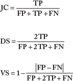
\begin{matrix} J C = \frac{T P}{F P + T P + F N} \\ D S = \frac{2 T P}{F P + 2 T P + F N} \\ V S = 1 - \frac{| F P - F N |}{F P + 2 T P + F N} \end{matrix}

TP (true positive) is the number of tumor voxels belonging to both the ground truth and simulated result; FP (false positive) is the number of tumor voxels belonging to the simulated result but not found in ground truth; and FN (false negative) is the number of tumor voxels belonging to ground truth but not found in the simulated tumor. For eliminating noise and artifacts, we set the detection threshold as 10% of the maximum value for both ground truth and the test datasets.

The evaluation metrics enable comparing the vasculature of the simulated tumor and the K^trans of the real FUI tumor, concerning their volumes. A cross-correlation analysis was made in order to further evaluate their internal transdifferentiations beyond size.

Results

Our method was applied to real patient data chosen from a nonresponder to therapy where the tumor was expanding, in order to approximate as much as possible free evolution. It is important to stress that it is hard to find patients without resection or untreated GBM for the entire duration of the disease. In this feasibility study, data were from a patient with two time points of DCE-MR images; the diagnostic and the FU clinical examinations were 39 days apart.

The clinical data used was taken from a patient with recurrent GBM, classified as stable disease using the Response Assessment in Neuro-Oncology (RANO) criteria, which is currently the clinical standard in the radiological FU of high-grade glioma patients. The data were taken from an imaging study approved by the local ethics committee of the University Hospitals Leuven, Leuven, Belgium. The DCE-MRI were acquired with a 3.0 T scanner (Achieva, Philips Medical Systems) using an é-channel head coil for reception and the body coil for transmission.

The presence of new lesions and the generalized tumor volume progression make this case appropriate for our study. The central necrotic lesions are located in the right frontal lobe. There is extensive edema, causing mass effect on the frontal horn of the right lateral ventricle.

Spatial Evolution of the Tumor and its Microenvironment

Figure 4 illustrates indicative simulation results after initializing vasculature and cell densities according to the described procedure. An analytic, quantitative evaluation of our modeling results that considers the 3D volume will be presented in the following paragraphs. An exemplar slice of the original K^trans map of the FU examination, which was performed 39 days after the initial examination, is also presented in Figure 4 for comparison. Within the frame of Figure 4 are illustrated the spatial distributions of the predicted vasculature (v) of the FUI, the normoxic (c), hypoxic (h), and necrotic (h) cell densities, as well as the angiogenic factors (a) after 39 fictitious days. The tumor increases in size, while hypoxic cells maintain the larger space within the tumor, and hypoxia-driven angiogenic factors are homogeneously allocated inside this hypoxia-bounded area. The predicted vasculature (v) is similar in shape with the actual FU of the K^trans map, and the model seems to qualitatively predict the hot spots of maximum abnormal vascularity (yellow to red intensity peaks). Such hot spots are usually important markers for the temporal therapeutic assessment and for therapy planning in general.

Figure 4

(Left) 57th slice with the K^trans map extracted from the real dataset of the FU1 session. (Within the frame) The simulated concentrations v, c, h, n, a of vasculature, normoxic cells, hypoxic cells, necrotic cells, and angiogenic factors, respectively.

Vasculature Predictions Correlated with K^trans map

The scatter plot of the K^trans map of the FUI image and the associated vasculature profile of the in silico approximation is shown in Figure 5. Higher values of either K^trans or vasculature density are expected at lower frequencies within a tumor mass. The calculated correlation coefficient is R = 0.8861, after truncating all zero values for K^trans and v. Taken together, the evaluation results show that the two tumors are strongly correlated both in terms of size and internal characteristics.

Figure 5

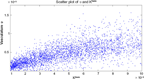
Scatter plot of K^trans against vasculature.

Vasculature Predictions Affected by D, ρ, and the Proliferative Rim

This section examines the effect of a number of critical modeling parameters on the simulation result, while quantitative metrics are used in order to better evaluate the outcome of the presented feasibility study. The first parameter studied was the diffusion coefficient D of tumor cells. Specifically, we explore how the simulated vasculature is affected when changing the diffusion rate of cells. Figure 6 shows the predicted spatial distribution of v for 0.1D and 10D, where D = 3.6 × 10^–8 cm²/s (Table 1) is within the range of values in relevant literature.³⁵ For comparison, Figure 6 also shows the original K^trans map of the FU examination as well as the predicted v for the original value of D. As expected, the pattern of v for low D is highly saturated, as the inability of tumor cells to migrate fast increases their local densities and consequently their demands for new vasculature. On the other hand, higher values of D result in an increase in tumor size and produce a pattern where the vasculature seems more extended and scattered than the original corresponding data of K^trans. A quantitative comparison has been also performed and presented in the next section.

Figure 6

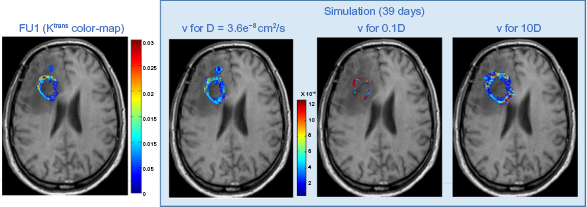
Effect of the different values of the diffusion coefficient D on the resulting vasculature.

The next step is to study the effect of the proliferation rate ρ to the results. Figure 7 shows how results differ for 0.1ρ and 10ρ, where ρ = 0.0087/day (Table 1) agrees with bibliography values.^{36, 52} The pattern of v for high ρ (ie, cells divide faster) shows a saturation of v, as increased cellular proliferation leads to increased tumor densities and metabolic demands that stimulate increase in vasculature. On the other hand, lower ρ produces a pattern where the vasculature seems more dispersed. Different values for both D and ρ were also tested (data not shown), but none reflected better the real FUI than the pair of values finally chosen.

Figure 7

Effect of the different values of the proliferation rate ρ on the resulting vasculature.

In summary, we present a quantitative evaluation of the agreement between the simulated tumor and the final tumor vasculature.

Table 2 presents the resulting metrics for different cases of parameters. Metrics regarding the uniform initialization of vasculature (uniform v) is noted, since it is commonly used in the absence of relevant information.³⁶ The scores for uniform vasculature are remarkably lower than the rest of the cases. Additionally, multiple erosions with different morphological operators were tried regarding the configuration of the area of the proliferative ring. However, this is not the case for the erosion of the necrotic core since the chosen erosion is representative of the population of cells changing between necrotic and hypoxic areas. Normoxic area diameter varied from 0 mm (no erosion) to ~10 mm (minimum hypoxia). As can be seen in Table 2, all metric scores are inversely proportional to the normoxic area expansion (erosions 1–5 mm show minimal differences). Alternatively, the less the assumed hypoxic region by erosion, the more inaccurate the model predictions become. According to our trials, the erosion of 1 mm appears to be the most appropriate. The parameters used in our approximation were selected to produce the highest scores for all three evaluation metrics.

Table 2.

Evaluation metrics of vasculature (%).

Temporal Evolution of the Tumor

Figure 8 shows the concentrations of the normoxic, hypoxic, and necrotic subpopulations over time. The total tumor population consisting of the sum of normoxic, hypoxic, and necrotic cells follows a Gompertzian-like growth, where an initially fast growth is followed by a slow-down phase. The normoxic subpopulation slightly decreases over time until it almost stabilizes, while hypoxic cells initially increase fast and then slow down where a plateau is reached. Furthermore, a slight increase of the necrotic population over time is also observed. As can be seen in Figure 8, hypoxic cells dominate within the tumor, indicating that oxygen supply is insufficient for the increasing metabolic demands of tumor cells. All populations start from a nonzero value determined by the initialization process.

Figure 8

Growth curves of the simulated concentrations c, h, n and the entire tumor (c + h + n) computed on the whole three-dimensional grid. Vertical axis is the non-dimensionalized concentration, and horizontal axis is time (days).

Figure 9 shows the evolution of vasculature and angiogenic factors over time. These biological phenomena are causally related; hypoxia leads to the expression of angiogenic factors, which in turn promote angiogenesis and the formation of vasculature in hypoxic areas. Note that, a few days after hypoxic cells start increasing (Fig. 8), both the levels of angiogenic factors and vasculature are rapidly multiplied (day 12 in Fig. 9). However, as hypoxic cells reach a plateau, the concentration of angiogenic factors is stabilized and vasculature keeps increasing.

Figure 9

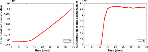
Growth curves of the simulated vasculature (left) and angiogenic factors (right) computed on the whole three-dimensional grid. Vertical axis is the normalized concentration, and horizontal axis is time (days).

As stated previously, the initial density of angiogenic factors, a₀, was set to zero. Once again, this model parameter was checked for values other than zero: particularly, a₀ was alternatively set to the maximum value of 1. Initially a steep drop by approximately three orders of magnitude of the angiogenic factors is observed as their consumption relative to their production is significantly higher (Fig. 10). However, as the tumor evolves and hypoxia increases, an increase in the angiogenic factors is also observed similar to that of Figure 9 (left). Interestingly, the resulting graphs of the three tumor populations and the overall tumor growth, as well as the growth of endothelial cells in time, appear to be almost the same as in Figures 8 and 9 (left). This indicates that the choice of initial a does not substantially affect the model's outcome.

Figure 10

Growth curve of the simulated angiogenic factors for a₀ = 1. A zoom of the phase after the steep drop (day 3) of the concentration of angiogenic factors is also shown.

Discussion

This paper focuses on predicting the evolution of the GBM tumor vascularization and presents a method that, in essence, is a feasibility study toward this difficult task. Models efficiently predicting vasculature are potentially of great interest, as the evolution of tumor growth is highly determined by the evolution of its vascularization, in the context of novel treatment strategies targeting angiogenesis and therapeutic decision making as well as predicting response to treatment.

DCE-MRI is a plausible clinical examination, while TM is the most common approach for Gd distribution estimations; hence, the significance of translating and subsequently using DCE-MRI to introduce multiple tumor development variables is evident. We presented a new way for defining the model inputs (image areas of interest and vasculature) of a glioma model by using biomarkers extracted by DCE-MRI, and demonstrated that it is feasible to predict vascularity despite the complexity of the model variables (Equations 1–6) and the assumptions made. In contrast to an arbitrary initialization with homogeneous vasculature as model input, we showed that the imaging-derived information regarding the initial vessel localization can yield more accurate results with respect to both tumor growth and vascularization predictions. The estimated spatial information of vasculature density within the ROI enables the model to predict intraregional differences that are closer to the ground truth. More interestingly, the method indicated that vascularity hot spot could be predicted, which in turn might be an important result for choosing the right therapy for the right patient.

Although we presented a number of qualitative and quantitative results on this study, also perturbing the parameters and the image areas of interest, the presented results need to be validated in a large number of patients in order to provide enough evidence that vasculature can be predicted with a standardized set of parameters and heuristics. In this respect, a sensitivity-specificity analysis would define a range of values within a patient database for the model parameters taken into account.³⁵

However, there is a difficulty in finding GBM patient data were the tumor evolution is unaffected from treatment, which renders this necessary validation hard. This represents a limitation of our model, since the actual therapeutic regimes (chemotherapy and radiotherapy) were not modeled in the current version. Use of the linear quadratic (LQ) model^{20, 22} could be in the direction for simulating radiotherapy, but the estimation of radiobiology parameters of the LQ is, however, the most challenging part of this task. We need to stress that, in order for this prediction method to reach the clinical setting, it will be also essential to model the effects of therapy.

An alternative prospect is to use additional imaging biomarkers in order to approximate other model parameters using either other MRI techniques, PET, or magnetic resonance spectroscopic imaging (MRSI). As an example, using diffusion MRI data, registered with the DCE MRI data, could also provide measures of cellularity to input the models.

A limitation of our method is that we oversimplified the discrimination of normoxic and hypoxic areas within the tumor. However, as a future perspective, determining these areas based on K^trans and/or other PK parameter values or even additional imaging modalities can be more accurate and representative of the reality. Alternatively, a control experiment could be used in order to determine the threshold value of K^trans in each image area. According to this procedure, a range of values would be assigned to a given area and the ROI divisions could be based on clustering the K^trans values.

Conclusion

The presented method focuses on vascularity prediction in GBM based on DCE-MRI data. The open challenges for patients with GBM and brain cancer in general are to find the right way of decoding MRI scans and obtain knowledge about the specific grade, characteristics, appropriate treatment, and patient response and probability of survival, all these from the very first moment that the cancer is diagnosed.

Our method, based on initializing a glioma model using DCE-MRI biomarkers, indicates that the 4D profile of vasculature can be predicted especially in the sense that it can prompt the clinician to regions were vascularity will reach very high K^trans values indicating tumor progression. Individualized predictions to monitor therapeutic effect and tumor development using computational models with noninvasive imaging biomarkers as input should be further investigated and validated, targeting direct clinical impact. This paper, however, presented a method for introducing vasculature in the modeling process, and this, if confirmed with large patient cohorts, can have a significant impact in predicting early the therapeutic effect especially with respect to tumor vasculature change. Clearly, the lack of proper retrospective patient data and the added computational requirements for calculating MRI-based vasculature maps are some of the obstacles and limitations to achieve larger scale verification. However, the potential benefit in predicting vasculature response can certainly outweigh these limitations and lead to the design of proper trials, which will also take into consideration patient clinical data such as gender, weight, and comorbidities, which have an effect on the computation of PK parameters and can therefore increase accuracy.

Another potential clinically relevant implementation of our method could be the prediction of a downstaging cancer as a result of a wider variety of factors, apart from radiotherapy. If this is the case, an operable GBM tumor could be identified in time, which would lead to improvement of clinical symptoms.

Author Contributions

Conceived and designed the experiments: AR, ET. Analyzed the data: MEO, ET, EK, SVC. Wrote the first draft of the manuscript: AR, MEO. Contributed to the writing of the manuscript: ET, EK. Agreed with manuscript results and conclusions: VS, KM. Jointly developed the structure and arguments for the paper: MEO, AR. Made critical revisions and approved final version: KM, VS. All authors reviewed and approved of the final manuscript.

References

Ali-Osman

Brain Tumors. Totowa, NJ: Humana Press; 2005.

Schiffer

Brain Tumor Pathology: Current Diagnostic Hotspots and Pitfalls. Dordrecht: Springer; 2006.

Goffart

, Kroonen

, Rogister

Glioblastoma-initiating cells: relationship with neural stem cells and the micro-environment.

Cancers. 2013; 5(3): 1049–71.

Krex

, Klink

, Hartmann

. German Glioma Network. Long-term survival with glioblastoma multiforme. Brain. 2007; 130(pt 10): 2596–606.

Zada

, Bond

A.E.

, Wang

Y.P.

, Giannotta

S.L.

, Deapen

Incidence trends in the anatomic location of primary malignant brain tumors in the United States: 1992–2006.

World Neurosurg 2012; 77(3-4): 518–24.

Hou

L.C.

, Veeravagu

, Hsu

A.R.

, Tse

V.C.

Recurrent glioblastoma multiforme: a review of natural history and management options.

Neurosurg Focus. 2006; 20(4): E5.

Lee

E.J.

, Ahn

K.J.

, Lee

E.K.

, Lee

Y.S.

, Kim

D.B.

Potential role of advanced MRI techniques for the peritumoural region in differentiating glioblastoma multiforme and solitary metastatic lesions.

Clin Radiol. 2013; 68(12): e689–97.

Tsougos

, Svolos

, Kousi

. Differentiation of glioblastoma multiforme from metastatic brain tumor using proton magnetic resonance spectroscopy, diffusion and perfusion metrics at 3 T. Cancer Imaging. 2012; 12: 423–36.

Flynn

J.R.

, Wang

, Gillespie

D.L.

. Hypoxia-regulated protein expression, patient characteristics, and preoperative imaging as predictors of survival in adults with glioblastoma multiforme. Cancer. 2008; 113(5): 1032–42.

10.

McNamara

M.G.

, Sahebjam

, Mason

W.P.

Emerging biomarkers in glioblastoma.

Cancers. 2013; 5(3): 1103–19.

11.

Zetter

B.R.

The scientific contributions of M. Judah Folkman to cancer research.

Nat Rev Cancer. 2008; 8(8): 647–54.

12.

Korkolopoulou

, Patsouris

, Konstantinidou

A.E.

. Hypoxia-inducible factor 1alpha/vascular endothelial growth factor axis in astrocytomas. Associations with microvessel morphometry, proliferation and prognosis. Neuropathol Appl Neurobiol. 2004; 30(3): 267–78.

13.

Daub

J.T.

, Merks

R.M.

A cell-based model of extracellular-matrix-guided endothelial cell migration during angiogenesis.

Bull Math Biol. 2013; 75(8): 1377–99.

14.

Zaman

M.H.

, Trapani

L.M.

, Sieminski

A.L.

. Migration of tumor cells in 3D matrices is governed by matrix stiffness along with cell-matrix adhesion and proteolysis. Proc Natl Acad Sci USA. 2006; 103(29): 10889–94.

15.

Mammoto

, Jiang

, Panigrahy

, Kieran

M.W.

, Mammoto

Role of collagen matrix in tumor angiogenesis and glioblastoma multiforme progression.

Am J Pathol. 2013; 183(4): 1293–305.

16.

Hanahan

, Weinberg

R.A.

Hallmarks of cancer: the next generation.

Cell. 2011; 144(5): 646–74.

17.

Hatzikirou

, Deutsch

Cellular automata as microscopic models of cell migration in heterogeneous environments. In: Santiago Schnell

PKMSAN

, Timothy

J.N.

eds. Current Topics in Developmental Biology. Vol. 81. Academic Press; 2008: 81.

18.

Lowengrub

J.S.

, Frieboes

H.B.

, Jin

. Nonlinear modelling of cancer: bridging the gap between cells and tumours. Nonlinearity. 2010; 23(1): R1.

19.

Stamatakos

G.S.

, Antipas

V.P.

, Uzunoglu

N.K.

, Dale

R.G.

A four-dimensional computer simulation model of the in vivo response to radiotherapy of glioblastoma multiforme: studies on the effect of clonogenic cell density.

Br J Radiol. 2006; 79(941): 389–400.

20.

Roniotis

, Marias

, Sakkalis

, Manikis

G.C.

, Zervakis

Simulating radiotherapy effect in high-grade glioma by using diffusive modeling and brain atlases.

J Biomed Biotechnol. 2012; 2012: 715S12.

21.

Clatz

, Sermesant

, Bondiau

P.Y.

. Realistic simulation of the 3-D growth of brain tumors in MR images coupling diffusion with biomechanical deformation. IEEE Trans Med Imaging. 2005; 24(10): 1334–46.

22.

Jbabdi

, Mandonnet

, Duffau

. Simulation of anisotropic growth of low-grade gliomas using diffusion tensor imaging. Magn Reson Med. 2005; 54(3): 616–24.

23.

Swanson

K.R.

, Alvord

E.C.

Jr , Murray

J.D.

A quantitative model for differential motility of gliomas in grey and white matter.

Cell Prolif. 2000; 33(5): 317–29.

24.

Roniotis

, Sakkalis

, Karatzanis

, Zervakis

M.E.

, Marias

In-depth analysis and evaluation of diffusive glioma models.

IEEE Trans Inf Technol Biomed. 2012; 16(3): 299–307.

25.

Roniotis

, Manikis

G.C.

, Sakkalis

, Zervakis

M.E.

, Karatzanis

, Marias

High-grade glioma diffusive modeling using statistical tissue information and diffusion tensors extracted from atlases.

IEEE Trans Inf Technol Biomed. 2012; 16(2): 255–63.

26.

Yankeelov

T.E.

, Atuegwu

, Hormuth

. Clinically relevant modeling of tumor growth and treatment response. Sci Transl Med. 2013; 5(187): 187–9.

27.

Baldock

A.L.

, Rockne

R.C.

, Boone

A.D.

. From patient-specific mathematical neuro-oncology to precision medicine. Front Oncol. 2013; 3: 62.

28.

Tofts

P.S.

, Kermode

A.G.

Measurement of the blood-brain barrier permeability and leakage space using dynamic MR imaging. 1. Fundamental concepts.

Magn Reson Med. 1991; 17(2): 357–67.

29.

Swanson

K.R.

, Rostomily

R.C.

, Alvord

E.C.

Jr . A mathematical modelling tool for predicting survival of individual patients following resection of glioblastoma: a proof of principle. Br J Cancer. 200S; 98(1): 113–9.

30.

Ellingson

B.M.

, LaViolette

P.S.

, Rand

S.D.

. Spatially quantifying microscopic tumor invasion and proliferation using a voxel-wise solution to a glioma growth model and serial diffusion MRI. Magn Reson Med. 2011; 65(4): 1131–43.

31.

Szeto

M.D.

, Chakraborty

, Hadley

. Quantitative metrics of net proliferation and invasion link biological aggressiveness assessed by MRI with hypoxia assessed by FMISO-PET in newly diagnosed glioblastomas. Cancer Res. 2009; 69(10): 4502–9.

32.

Swanson

K.R.

, Chakraborty

, Wang

C.H.

. Complementary but distinct roles for MRI and 18F-fluoromisonidazole PET in the assessment of human glioblastomas. J Nucl Med. 2009; 50(1): 36–44.

33.

Atuegwu

N.C.

, Arlinghaus

L.R.

, Li

. Parameterizing the logistic model of tumor growth by DW-MRI and DCE-MRI data to predict treatment response and changes in breast cancer cellularity during neoadjuvant chemotherapy. Transl Oncol. 2013; 6(3): 256–64.

34.

Leach

M.O.

, Brindle

K.M.

, Evelhoch

J.L.

. Pharmacodynamic/Pharmacokinetic Technologies Advisory Committee, Drug Development Office, Cancer Research UK. The assessment of antiangiogenic and antivascular therapies in early-stage clinical trials using magnetic resonance imaging: issues and recommendations. Br J Cancer. 2005; 92(9): 1599–610.

35.

Swanson

K.R.

, Rockne

R.C.

, Claridge

, Chaplain

M.A.

, Alvord

E.C.

Jr , Anderson

A.R.

Quantifying the role of angiogenesis in malignant progression of gliomas: in silico modeling integrates imaging and histology.

Cancer Res. 2011; 71(24): 7366–75.

36.

Hinow

, Gerlee

, McCawley

L.J.

. A spatial model of tumor-host interaction: application of chemotherapy. Math Biosci Eng. 2009; 6(3): 521–46.

37.

Tzamali

, Favicchio

, Roniotis

. Employing in-vivo molecular imaging in simulating and validating tumor growth. Conf Proc IEEE Eng Med Biol Soc. 2013; 2013: 5533–6.

38.

Hubbard

M.E.

, Byrne

H.M.

Multiphase modelling of vascular tumour growth in two spatial dimensions.

J Theor Biol. 2013; 316: 70–89.

39.

Bartha

, Rieger

Vascular network remodeling via vessel cooption, regression and growth in tumors.

J Theor Biol. 2006; 241(4): 903–18.

40.

Gevertz

J.L.

, Torquato

Modeling the effects of vasculature evolution on early brain tumor growth.

J Theor Biol. 2006; 243(4): 517–31.

41.

Frieboes

H.B.

, Jin

, Chuang

Y.L.

, Wise

S.M.

, Lowengrub

J.S.

, Cristini

Three-dimensional multispecies nonlinear tumor growth-II: Tumor invasion and angiogenesis.

J Theor Biol. 2010; 264(4): 1254–78.

42.

Thompson

, Mills

S.J.

, Coope

D.J.

, O'Connor

J.P.

, Jackson

Imaging biomarkers of angiogenesis and the microvascular environment in cerebral tumours.

Br] Radiol. 2011; 84(Spec No 2): S127–44.

43.

Harrer

J.U.

, Parker

G.J.

, Haroon

H.A.

. Comparative study of methods for determining vascular permeability and blood volume in human gliomas. J Magn Reson Imaging. 2004; 20(5): 748–57.

44.

Barker

P.B.

, Golay

, Zaharchuk

, eds. Clinical Perfusion MRI. Cambridge University Press; 2013.

45.

Turkbey

, Kobayashi

, Ogawa

, Bernardo

, Choyke

P.L.

Imaging of tumor angiogenesis: functional or targeted?

Am J Roentgenol. 2009; 193(2): 304–13.

46.

Jackson

, O'Connor

J.P.

, Parker

G.J.

, Jayson

G.C.

Imaging tumor vascular heterogeneity and angiogenesis using dynamic contrast-enhanced magnetic resonance imaging.

Clin Cancer Res. 2007; 13(12): 3449–59.

47.

Wachspress

E.L.

, Habetler

G.J.

An alternating-direction-implicit iteration technique.

J Soc Indust Appl Math. 1960; 8(2): 403–23.

48.

Douglas

J.J.

Alternating direction methods for three space variables.

Numerische Math. 1962; 4(1): 41–63.

49.

Neal

M.L.

, Trister

A.D.

, Cloke

. Discriminating survival outcomes in patients with glioblastoma using a simulation-based, patient-specific response metric. PLoS One. 2013; 8(1): e51951.

50.

Freyer

J.P.

, Sutherland

R.M.

Regulation of growth saturation and development of necrosis in EMT6/R0 multicellular spheroids by the glucose and oxygen supply

Cancer Res. 1986; 46(7): 3504–12.

51.

Mueller-Klieser

Method for the determination of oxygen consumption rates and diffusion coefficients in multicellular spheroids.

Biophys J. 1984; 46(3): 343–8.

52.

Hegedus

, Czirok

, Fazekas

, B'Abel

, Madar'asz

, Vicsek

Locomotion and proliferation of glioblastoma cells in vitro: statistical evaluation of videomicroscopic observations.

J Neurosurg. 2000; 92(3): 428–34.

A Proposed Paradigm Shift in Initializing Cancer Predictive Models with DCE-MRI Based PK Parameters: A Feasibility Study

Abstract

Keywords

Introduction

Methods

PK DCE-MRI Parameters

Tumor Areas Defined by Ktrans

Vasculature Defined by Ktrans

Computational Model of Tumor Growth

Stepping from ROI to Discrete Tumor Areas

Model Initialization and Parameterization

Quantitative Metrics for Spatial Evaluation

Results

Spatial Evolution of the Tumor and its Microenvironment

Vasculature Predictions Correlated with Ktrans map

Vasculature Predictions Affected by D, ρ, and the Proliferative Rim

Temporal Evolution of the Tumor

Discussion

Conclusion

Author Contributions

References

Tumor Areas Defined by K^trans

Vasculature Defined by K^trans

Vasculature Predictions Correlated with K^trans map