Sage Journals: Discover world-class research

Abstract

Recently, new but expensive treatments have become available for metastatic melanoma. These improve survival, but in view of the limited funds available, cost-effectiveness needs to be evaluated. Most cancer cost-effectiveness models are based on the observed clinical events such as recurrence-free and overall survival. Times at which events are recorded depend not only on the effectiveness of treatment but also on the timing of examinations and the types of tests performed. Our objective was to construct a microsimulation model framework that describes the melanoma disease process using a description of underlying tumor growth as well as its interaction with diagnostics, treatments, and surveillance. The framework should allow for exploration of the impact of simultaneously altering curative treatment approaches in different phases of the disease as well as altering diagnostics. The developed framework consists of two components, namely, the disease model and the clinical management module. The disease model consists of a tumor level, describing growth and metastasis of the tumor, and a patient level, describing clinically observed states, such as recurrence and death. The clinical management module consists of the care patients receive. This module interacts with the disease process, influencing the rate of transition between tumor growth states at the tumor level and the rate of detecting a recurrence at the patient level. We describe the framework as the required input and the model output. Furthermore, we illustrate model calibration using registry data and data from the literature.

Keywords

melanoma microsimulation modeling tumor growth cancer progression

Introduction

Melanoma incidence is rising worldwide. In the Netherlands, the incidence per 100,000 went up from 12.8 in 2001 to 19.7 in 2011 (world-standardized rate) and mortality increased by 44%.¹ Worldwide, over 55,000 people died from melanoma in the year 2012.² Most melanoma patients are diagnosed with local disease and treated with resection of the primary tumor only. Most of these patients are then cured, but about 15% will develop one or more recurrences.³ Until a few years ago, treatment options for (distant) metastatic melanoma were limited, and three-year overall survival (OS) was only about 15%.⁴ In the past few years, the number of treatment options for metastatic melanoma has increased with immunotherapeutic drugs such as ipilimumab and nivolumab and targeted drugs such as BRAF and MEK inhibitors. These expensive drugs greatly improve survival for subgroups of patients, but in view of the limited funds available, cost-effectiveness needs to be evaluated.^5–7 In addition, expensive forms of diagnostics such as next-generation sequencing and FDG-PET-CT are becoming available. It is important to evaluate whether it would be cost-effective to include these diagnostics in the care for melanoma and whether the timing of their use in the disease process may be optimized.

To evaluate cost-effectiveness in cancer, Markov-type mathematical models are often used.^8–11 Health states in these models are usually based on the observed clinical states. In cancer treatment, these are primary tumor, local and regional recurrence, distant metastasis, and death.^12–15 The times at which patients remain in these states are equivalent to recurrence-free survival (RFS), distant recurrence-free survival (DRFS), progression-free survival (PFS), disease-specific survival (DSS), and OS. Times at which clinical states are observed, however, largely depend on the timing of examinations and the choice of diagnostic tests.

Most cost-effectiveness models in oncology do not attempt to model the whole disease and care pathway, but only compare interventions within a single-treatment line. When a new treatment is evaluated, the surveillance schedule, imaging techniques, and other tests are kept same. If one of these change, the model would need to be redone. A better solution would be to construct a model of underlying disease including an overlay of diagnostic testing that can be applied at adjustable intervals. Such models already exist for another aspect of cancer care, namely, screening.^16–19 These models simulate the underlying tumor growth or their precursors and interact with the screening models, in which frequency and timing of testing, test characteristics, and follow-up procedures are specified. However, such models do not exist for disease progression and care after diagnosis. Although models including the whole cancer treatment pathway exist,^20,21 a description of the underlying disease is required to investigate the full impact of new diagnostics, treatments, follow-up, and downstream treatment effects. For recurrence and surveillance of colorectal cancer (CRC), a modeling approach roughly comparable with the approaches used in cancer screening has been applied by Rose et al.²²

For melanoma, we present in this study the development of a framework based on underlying tumor growth; MAICare -an acronym for “Microsimulation for the Assessment of Individualized Cancer Care”. The model allows for studying the effects of altering complex patterns of care in melanoma. We describe the structure and the required parameters of the model, the underlying assumptions, and the calibration procedure. Finally, we present the results of a first calibration of the model using the available Dutch and German data.

Methods

Model Framework

We developed a microsimulation framework to simulate the progression of melanoma. Essentially, health trajectories of individual melanoma patients are simulated from first diagnosis until death. The framework is structured in such a way that it can be adjusted to different treatments, altered surveillance schemes, and new diagnostics. It consists of two components, namely, the disease model and the clinical management module (Fig. 1). The model has been coded in C++ and has a Microsoft Excel user interface.

Figure 1

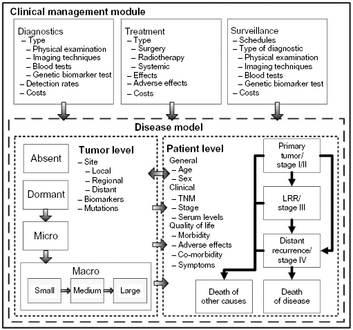
Structure of the model framework. The model consists of two components, a disease model and a clinical management module. The disease is modeled at two levels, including the level of the tumor and the level of the patient. The tumor level describes the progression of disease, the patient level, the clinical observed states, and the quality of life. The clinical management module consists of the interventions in the disease process, consisting of diagnostic techniques, treatments, and surveillance strategies.

Disease Model

The disease model is composed of two levels: the tumor level and the patient level. The tumor level describes underlying, and often unobservable, tumor growth and metastasis. The patient level contains clinically observable events such as recurrence of disease, progression, and death. The former level is nested within the patient level, and the two levels of the disease model interact. For example, size and location at the tumor level influence the chance to become symptomatic and, as such, be diagnosed with recurrent disease.

Tumor Level

Tumor growth is largely unobservable, but increasingly more is known about the process of growth, progression, and metastasis. We modeled tumor growth according to the current theory of rate-limiting steps (Fig. 2).^23–27 Tumor growth is simulated via three Markov chains, indicating recurrence on the local recurrence site, on regional sites, and progression and metastasis on distant sites, in agreement with the TNM staging classification.⁴ Local recurrence denotes the growth of a tumor within 4 cm of the primary tumor. Regional recurrence indicates the growth of one or more metastases in the regional lymph nodes. Distant recurrence indicates the growth of one or more metastases at distant sites and/or organs. Growth of tumors on local, regional, and distant recurrence sites are simulated in parallel.

Figure 2

The simulation cycle. Patients enter the model at first diagnosis, they then undergo additional diagnostic testing. If necessary, the stage is adjusted, and a treatment is selected and applied. This process is either completely successful, ie, all tumors and metastases have been detected and successfully treated, all tumor growth states are set to absent, and no tumor growth ensues. Or a metastasis is missed during the diagnostic process and/or a treatment is not completely successful, at least one tumor chain is set to the dormant or higher state and tumor growth ensues. At set intervals, surveillance has place, which entails the types of diagnostic tests that are done and their detection rates. This results in either detection of a recurrence, or no detection, after which tumor growth proceeds. If a tumor grows but remains undetected during surveillance, it will eventually become symptomatic and a recurrence is registered. After a recurrence has been registered, the cycle restarts. Patients undergo further diagnostic tests and receive treatment, and a surveillance strategy is applied.

Each Markov chain consists of the tumor growth states as follows: absent, dormant, micro, and macro. The absent state represents no tumor; the dormant state represents no demonstrable tumor, but circulating tumor cells; the micro state represents a small tumor without any vascularization (<2 mm); and the macro state represents a larger tumor with vascularization. To account for the fact that tumor detectability by imaging techniques depends on size, the macro state was divided into three sub states, ie, macro small (2–5 mm), medium (5–8 mm), and large (>8 mm). In time, a growing macro tumor will become symptomatic, also in the absence of diagnostic testing. Therefore, an additional tumor state was added, namely, macro symptomatic.

State transitions on the tumor level take place as follows. After initial diagnosis and treatment, there is the probability that a patient is cured from the disease. In that case, the three tumor chains are set to absent. If the patient is not (entirely) cured by treatment, the starting states of the tumor chains are drawn. There are four options such as follows: dormant on all three chains, and micro on one of the three chains while the remaining two chains are set to dormant. That is, at most on one chain, a micro tumor remains after treatment. Once the starting states for the tumor growth chains have been drawn, growth is simulated by a survival function. Parameters in the function are current tumor growth state, phase of disease (with the values stage I, stage II, stage III, local recurrence, and regional recurrence), and optionally additional patient features (see Appendix 1). Each transition between two tumor growth states is determined by a new random draw, and we assume that there is no correlation between transition times within or between chains. After each recurrence and treatment for this recurrence, the simulation of tumor growth is repeated.

Patient Level

The patient level of the disease model consists of the clinical disease phases that are used in practice to describe the extent and progression of disease in an individual patient. For melanoma, like in most cancer types, these are staged at initial diagnosis, ie, stages I, II, III, and IV, recurrence, ie, local, loco-regional, regional recurrence, and distant metastasis. In addition to the clinical disease phase, a patient has additional features, namely, sex, age, and WHO performance score.²⁸ These features may influence the tumor growth rate on the tumor level. Transitions on the patient level occur only indirectly, namely, when a growing tumor has become symptomatic or when tumor growth has been detected during surveillance in the clinical management module.

The final end point in the model is death. Death due to melanoma can occur only in patients with metastatic disease. From the moment of detection of a tumor on the distant chain, either by surveillance or by symptoms, time to death is drawn based on prognostic factors such as sex and age at diagnosis. The timing of death due to other causes is drawn, for each patient, at the start of the simulation. Death due to other causes depends on sex and age and is based on death rates published by Statistics Netherlands.²⁹ The simulated patient dies from the death cause that comes first in the model.

Note that there is no health state for cure of disease in the model. Patients may be classified as cured of disease, retrospectively, if there has been no recurrent disease after treatment during the remaining lifetime. Furthermore, note that by using this definition of cure of disease, the proportion of cured patients does not correspond with the proportion of individuals for whom all three tumor growth chains have been reset to the absent state after treatment. After all, a patient in whom the tumor growth states have been set to dormant after treatment may not experience a recurrence within their lifetime.

Clinical Management Module

The clinical management module consists of a diagnostics, treatment, and surveillance segment. In contrast to the disease model, parameters and schedules in the clinical management module can be changed by the ones used to simulate different healthcare scenarios.

Diagnostics

The diagnostic segment specifies which diagnostic tests are used and at which time point. It includes a list of possible diagnostic techniques such as physical examination, imaging techniques, and sentinel lymph node biopsy (SLNB). Each test has detection and miss rates specific to each tumor growth state and recurrence site on the tumor level. These rates are based on the values found in the literature.^30–34

Treatment

Different types of treatment (surgery, radiotherapy, and drug therapy) can be specified in the model, as well as decision rules that govern the choice of treatment for a specific patient. As a result of treatment, the three tumor chains are (re)set. Resetting each chain is done according to a probability distribution that specifies the proportion of patients who transition to the absent or dormant state, or remain in an active (micro) state for each relevant treatment choice. For an individual, we denote the resulting set of states for the three tumor chains as the tumor starting state distribution. Once the starting states after treatment have been drawn, growth is simulated.

In addition to influencing the tumor starting state distribution, treatment choice may influence the tumor growth rate, ie, the rate of transitioning between consecutive tumor growth states. This influence takes the form of a hazard ratio (HR) that is added to the parametric time-to-event function, as described in Appendix 1. At present, care (and the corresponding disease progression) according to the current clinical guidelines is assumed in the model. That is, the HR for treatment in the time-to-event functions describing tumor growth is currently set to 1, indicating that current care is the reference strategy. To evaluate the comparative (cost-)effectiveness of an alternative treatment choice for a specific patient population, the HR relative to current care for that population is to be specified.

Surveillance

The surveillance segment specifies the decision rules that describe which test is applied when (see Appendix 2). A typical surveillance strategy states the time points at which surveillance takes place, the total number of surveillance visits planned, and the tests performed during surveillance. These strategies are specified separately for stage IA, stages IB–IIC, stage III, local recurrence, and regional recurrence, because guidelines and clinical practice data indicate that different intervals for surveillance visits and different diagnostic tests are used for different stages of the disease.

The detection of recurrent tumors that are present at the tumor level causes a transition in the health state of the individual at the patient level, with the particular health state depending on the site(s) of recurrent tumor(s). After initial detection of the recurrent tumor, further diagnostic testing and treatment for the recurrence or metastasis is initiated. The treatment upon detection of recurrence may be specified as a function of site of recurrence, previously administered treatments, and other features of the patient or the tumor, such as age, performance status, and genetic mutations. It is possible to specify the proportion of patients who refrain from treatment after the detection of a recurrence. This proportion may differ depending on the number of past treatments.

Simulation Cycle

Figure 2 depicts the simulation cycle, illustrating the order of the different simulation steps. Below we describe the clinical management module, with the relevant assumptions, inputs, and the output.

Patients enter the model at first diagnosis. A patient is generated by drawing sex, age, stage, and additional stage-specific characteristics such as presence of ulceration, according to (conditional) probabilities that are directly taken from routinely collected data from the Dutch cancer registry. Using data from Statistics Netherlands, time to death due to other causes is drawn, conditional upon sex and age at diagnosis.

Based on the patient characteristics, further diagnostic tests are selected, for example, like SLNB, and a treatment is assigned. Based on the test results and treatment, the starting states of the local, regional, and distant chain on the tumor level are drawn.

Subsequently, at the tumor level, tumor growth is simulated from the starting states drawn in the previous step, taking the impact of the choice of treatment on the tumor growth rates into account. There are two options as follows.

All three chains are in the absent state: No growth is simulated. The only transition to occur is death due to other causes (drawn during step 1).

The three chains are all in the dormant state or one of the three chains is in the micro tumor growth state. Growth is simulated based on the tumor growth model.

Based on the phase and the chosen treatment, a surveillance schedule is selected, in agreement with the Dutch guidelines. At each scheduled surveillance visit, detection rates of planned diagnostic tests are applied to a patients’ true underlying tumor state on each of the three chains. This may result in the detection of a recurrence or of progression of disease. Surveillance continues until the end of the surveillance schedule as specified in the clinical management module, until a recurrence is detected or until the death of other causes, whatever comes first. Note that, if not detected by surveillance, recurrent or progressive disease may also be detected through symptoms. This occurs when a patient enters the state symptomatic tumor on any of the three chains.

When a patient enters the recurrence state on the patient level, the type of recurrence is determined by the chain that first reached the symptomatic state, or in case of detection during surveillance the severest type of recurrence. In case of a local or regional recurrence, the patient goes back to step 2 and proceeds through the model as described in steps 2–5. In case of progression to metastatic disease, time to death of melanoma is drawn.

Further information about the implementation of the model, the user interface, and internal versus user-defined model parameters can be found in Appendix 3.

Model Parameters and MCMC Calibration Procedure

The model framework is specified by quantifying the following groups of parameters.

The parameters in the growth function that specify the rate of transitioning between the five tumor growth states dormant, micro, macro small, macro medium, and macro large and the decision rules for the choice of treatment.

The proportion of patients for whom the growth state at the tumor level is reset to absent, dormant, or micro.

The decision rules for the timing and the type of test applied during surveillance after treatment.

The test positivity rate for each test specified during diagnosis or surveillance, dependent on tumor state, site of the tumor, and other relevant patient and/or tumor features.^30–34

The parameter groups 3 and 4 are quantified on the basis of literature estimates, clinical guidelines, and real world data on clinical practice. Parameter groups 1 and 2 are essentially unobservable and cannot be quantified directly on the basis of patient data. Values for these parameters are obtained by calibration, in such a way that model predictions for a large sample of patients are in agreement with a number of observed targets. These targets are data on RFS, DRFS, PFS, and OS. Preferably these are obtained from patient-level data, but it is possible to use survival estimates from the literature as well.

To calibrate the group 1 and group 3 parameters, an automatic MCMC calibration procedure with rejection sampling was implemented.³⁵ As five different unobservable tumor states are included in the model, an infinite number of fitting parameter sets may be obtained and parameter values may not converge. To limit the number of fitting parameter sets and eliminate illogical parameter combinations, one restriction was added to the calibration procedure; the assumption that, on average, dwelling times in the macro growth states only decrease with larger sizes.³⁶ Thus, the hazard rate (HR) for the transition from micro to macro small, HRmicro–macro small, must be higher than HRdormant–micro. Likewise HRmacro small–macro medium must be higher than HRmicro–macro small, and HRmacro medium–macro large must be higher than HRmacro small–macro medium. This restriction did not apply to HRmacro large–symptomatic. An example of the resulting growth curve is depicted in Figure 3. The shape of the curve is broadly comparable with the Gompertzian growth curve described in the literature.³⁶

Figure 3

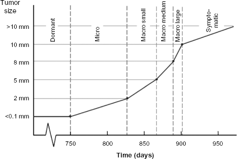
Tumor growth according to the rate - limiting steps theory. Tumor growth as it is currently simulated in the model, with example dwelling times (in days) for each tumor growth state.

The calibration procedure results in a prespecified number of parameter sets that all lead to model predictions in agreement with the calibration targets. These parameter sets can be used to simulate alternative treatment scenarios in such a way that a credible range for model-based outcomes can be obtained.

Model Assumptions

At present, the simulated population in the MAICare framework is the Dutch patient population, with baseline TNM staging and additional features as registered in the Dutch cancer registry between 2006 and 2011. Only one treatment arm, ie, current care, is currently simulated by the model. Decision rules for diagnostic testing, treatment, and surveillance were based on current Dutch guidelines. Sensitivities and specificities found in literature were transformed to detection and miss rates for the diagnostic tests and imaging techniques in the model.^37–39 We assumed that no local recurrence could occur after treatment in stage III, local recurrence, or regional recurrence. Thus, only two tumor chains (regional and distant) were simulated after stage III, namely, the regional and the distant chain.

Data for Calibration

With respect to OS, we used the stage-specific OS in Dutch melanoma patients from the Dutch Cancer Registry (2000–2012) as calibration data.¹ No data on time to recurrence are yet available for the Dutch melanoma patient population. However, detailed data on melanoma progression, stratified according to stage at diagnosis is available from a large German cohort.⁴⁰ These data were presently used to calibrate stage-specific RFS in the model, as well as OS after local, regional, and distant recurrence.^41,42 In addition, as a validation step, we compared the stage-specific OS to that of Dutch Registry data.¹

Analyses

The calibration of a microsimulation model is always an iterative process. In principle, the calibration was done in the stepwise fashion described below, but occasionally, we had to return to a previous step to achieve a better fit.

We established starting state distributions after treatment in accordance with literature and expert opinion. Also, we set the probabilities of detection for each surveillance test, based on literature and expert opinion.

We started a calibration round for the tumor growth parameters by fitting the stage I, II, and III RFS output of our model to RFS curves based on German data.⁴⁰ We carried out the calibration procedure with a patient population of size 250,000. Model fit for RFS was assessed at 6 months, and after that yearly up till 10 years after diagnosis. Based on discussions with clinical experts, we assumed a median dormancy state duration between 1.5 and 3 years and used this as an additional calibration target. We started with calibration of the tumor growth parameters scale and shape, the proportional hazards for phase of disease: stages I, II, and III at diagnosis (reference stage I) and the tumor growth transitions to micro (reference transition), macro small, macro medium, macro large, and symptomatic. We started the calibration algorithm using betas [ln(HR)] of zero as starting values. We ran the calibration procedure five times, to manage the correlation between draws. Parameter sets that resulted in a binomial deviance statistic of over 3.84 (P < 0.05) on any of the RFS targets over time were excluded.

We calibrated the parameters of the time to death of melanoma model that becomes active after diagnosis of metastatic disease. Calibration targets were again taken from German data and consisted of OS in stage IV/metastatic patients.^41,42 We calibrated the scale, shape, and the proportional hazards for M-status [M1a (reference), M1b, and M1c] in the same manner as we calibrated the tumor growth parameters.

Finally, we calibrated the model against the OS after a local or a regional recurrence.³ Model parameters that were calibrated in this step are the proportional hazards for phase of disease (local, recurrence, or regional recurrence) and the tumor starting state distribution after treatment for stage III or a regional recurrence.

After calibration to OS after local and regional recurrence, we checked whether stage-specific OS matched with that of Dutch Registry data. Because no satisfying fit was obtained, we systematically varied the tumor starting state distributions after treatment for stage III and after treatment for regional recurrence. The proportion of patients that started in the absent state was kept as in step 1 (0.35 for stage III, and 0.1 for regional recurrence), but the proportion of individuals in whom the tumor state was set to dormant, micro regional, and micro distant was varied. For these three proportions, both for stage III and for regional recurrence, a total of 1134 scenarios were explored. The only constraint was that the sum of three was 0.65 in stage III and 0.9 in regional recurrence. All analyses were run with a patient population of size 250,000.

Results

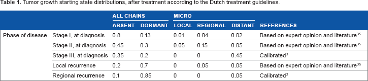
The tumor starting state distributions after treatment are shown in Table 1. Note again that these are mostly based on expert opinion. Only the tumor starting state distributions after treatment for stage III and after regional recurrence were obtained by calibration. The proportion of individuals with all tumor chains set to absent after treatment decreases considerably with the severity of disease phase. Particularly after treatment for recurrent disease, the chance to be free from any remaining tumors is small.

Table 1

Tumor growth starting state distributions, after treatment according to the Dutch treatment guidelines.

		ALL CHAINS		MICRO			REFERENCES
		ABSENT	DORMANT	LOCAL	REGIONAL	DISTANT	REFERENCES
Phase of disease	Stage I, at diagnosis	0.8	0.13	0.01	0.04	0.02	Based on expert opinion and literature³⁵
	Stage II, at diagnosis	0.45	0.3	0.05	0.15	0.05	Based on expert opinion and literature³⁵
	Stage III, at diagnosis	0.35	0.2	0	0	0.45	Calibrated³
	Local recurrence	0.2	0.7	0	0.05	0.05	Based on expert opinion and literature³⁵
	Regional recurrence	0.1	0.85	0	0	0.05	Calibrated³

The probabilities of detection per surveillance test, dependent on tumor site and growth state, can be found in Table 2.

Table 2

Probability of detection during surveillance.

TEST	TUMOR CHAIN	TUMOR GROWTH STATE					REFERENCES
TEST	TUMOR CHAIN	DORMANT	MICRO	MACRO S	MACRO M	MACRO L	REFERENCES
Physical examination	Local	0	0.2	0.5	0.7	1	Based on expert opinion
	Regional	0	0	0.1	0.3	0.8
	Distant	0	0	0	0.1	0.25
CT	Local	0	0.2	0.5	0.7	1	Based on literature^{29,30,31,32,33}
	Regional	0	0	0.1	0.3	0.8
	Distant	0	0	0	0.1	0.25

The best fitting set of parameters for the tumor growth model is given in Table 3. Mean tumor growth state transition times in stage I as predicted by this model are shown in Figure 3. Note that the shape of the curve is in agreement with the current theory of cancer growth according to rate-limiting steps.

Table 3

Tumor growth model.

MODEL TYPE	WEIBULL PH			REFERENCES
Shape		0.59		Calibrated³⁵
		Beta	HR^*
Constant		0.11	1.12	Calibrated³⁵
Phase of disease	Stage I, at diagnosis	0	1	Calibrated³⁵
	Stage II, at diagnosis	0.72	2.05
	Stage III, at diagnosis	1.42	4.15
	Local recurrence	0.2	1.22	Calibrated³
	Regional recurrence	0.8	2.23
Transition	Dorm → Micro	0	1	Calibrated³⁵
	Micro → Macro S	2.32	10.18
	Macro S → Macro M	4.55	94.49
	Macro M → Macro L	4.85	128.25
	Macro L → Sympt	1.12	3.06

HR = exp(beta).

Model fit with regard to RFS in stages I, II, and III for the best fitting set of parameters for the tumor growth model is shown Figure 4A, B, and C, respectively. The model-based predictions did not differ significantly from the German calibration data. The best fitting parameter set for the stage IV time-to death of melanoma model is shown in Table 4. Model fit with regard to stage IV/metastatic OS for M1a, M1b, and M1c is shown in Figure 4D, E, and F, respectively. Again model-based predictions did not differ significantly from the calibration data. With respect to OS after local recurrence and OS after regional recurrence, the difference between model predictions and the German calibration targets was again not statistically significant (figures not shown). Finally, model-based OS from diagnosis of stage I, II, and III and the corresponding Dutch cancer registry data are shown in Figure G, H, and I, respectively. Herein, model-based predictions did differ significantly from the data, because the sample size of the cancer registry data results in extremely small confidence intervals. Nevertheless, the predictions were reasonably close to the observed OS curves for the Netherlands.

Figure 4

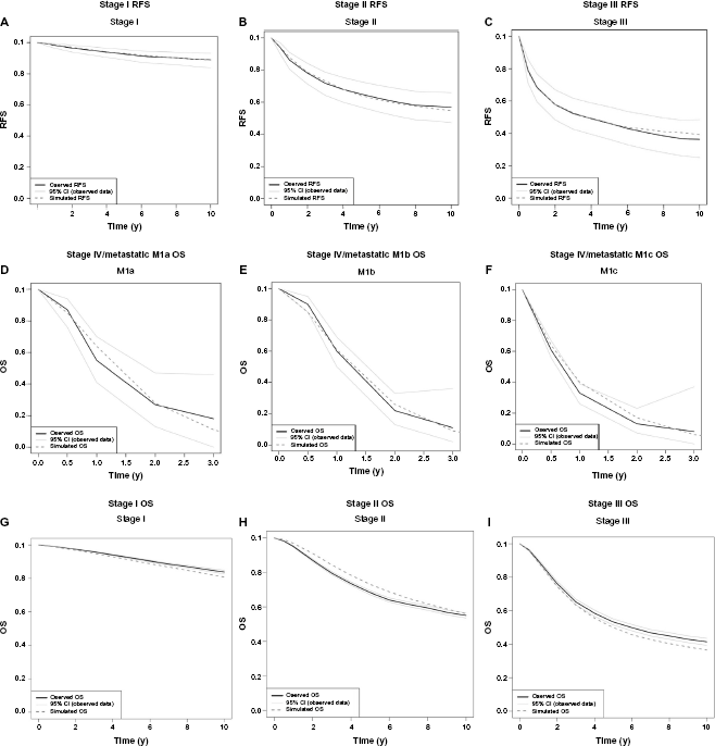
Model - based predictions for the best fitting parameter set, resulting from the calibration procedure and calibration data for different model outcomes. Solid black lines represent the data, light gray lines the 95% CI of the data, and the dark gray dashed lines the simulation model results. Figures 4A, B, and C show the model fit for RFS for stages I, II, and III, respectively. Figures 4D, E, and F show the model fit for OS for stages IV and metastatic M1a, M1b, and M1c, respectively. Figures 4G, H, and I show the model fit for OS for stages I, II, and III, respectively.

Table 4

Death of melanoma model.

MODEL TYPE	WEIBULL PH			REFERENCES
Shape		1.46		Calibrated^38,39
		Beta	HR^*
Constant		0.46	1.58	Calibrated^38,39
M status	M1a (soft tissue only)	0	1	Calibrated^38,39
	M1b (lung)	0.02	1.02
	M1c (other visceral)	1.87	6.49

HR = exp(beta).

Discussion and Conclusion

We have introduced a new modeling framework for simulating melanoma care and progression, MAICare, which stands for “Microsimulation for the Assessment of Individualized Cancer Care”. The framework was developed with a focus on melanoma care, but generalizability to other solid tumor types was a guiding principle during the development. We presented a calibration procedure to quantify the model and demonstrated that acceptable model predictions for a range of health outcomes can be achieved using literature-based summary statistics.

Parameter calibration is an approach used for many complex models in order to quantify internal, unobservable, model parameters. We carried out a first model calibration for the Dutch patient population. Because of a lack of Dutch data on intermediate outcomes, we used German data on RFS and OS after recurrence. In addition, we did not have patient-level data to our disposition, and as such, we were forced to make many simplifying assumptions. Nevertheless, we were able to calibrate the model such that model-based predictions for stage-specific OS closely approached Dutch registry data. For future use of the model in, for example, health-economic analyses, however, it is recommended to carry out a more detailed calibration using patient-level data specifically for the Dutch patient population. For this purpose, a large retrospective study in 1000 melanoma patients has been initiated. These data will deliver detailed information on number, location, and timing of consecutive recurrences, allowing full model calibration.

Another disadvantage of the present model is the fact that the stage IV/metastatic disease model is calibrated against care data from the years 1996 and 2010, as reported in the literature.⁴² This essentially means that the metastatic model reflects treatment with surgery, radiotherapy, and primarily dacarbazine; from start of treatment, only time to death from melanoma is simulated. Multiple treatment lines in the metastatic phase, with different consecutive drugs can presently not be simulated in the MAICare model. Nevertheless, the current model provides an appropriate reference strategy against which to explore the cost-effectiveness of new, expensive therapies such as BRAF inhibitors and immunotherapeutic drugs. Furthermore, in the near future, the model will be extended to include multiple treatment lines using the above-mentioned retrospective study as well as data from the recently initiated prospective Dutch melanoma treatment registry.⁴³

The strength of our framework is the fact that we modeled the disease process not only on a patient level but also on a tumor level, describing the growth and metastasis of tumors in different locations. In addition, we included a separate clinical management module that interacts with this disease process. This model structure makes it possible to explore the impact of simultaneously altering two or more interventions in the care process. Furthermore, it is possible to assign molecular features to the tumor chains, such that the model may also be used to generate hypotheses concerning the potential impact of molecular diagnostics in combination with targeted treatments. For example, we envisage exploration of the potential value of next-generation sequencing and subsequent adaptation and personalization of treatment within the adjuvant or metastatic setting.

The analysis of multiple interventions is useful for the optimization of the whole care pathway. Especially when new interventions have high incremental costs, it may be helpful to modify care on more than one point. For example, many of the new cancer treatments for metastatic disease show some beneficial effects, but are expensive and response durations are limited due to acquired tumor resistance. During treatment with these drugs, patients are under surveillance, and usually a CT scan is done every three months. If tumor progression is detected, the drug treatment is stopped. It has been suggested that surveillance using molecular imaging tests, such as FDG-PET-CT scans, with shorter time intervals, would allow for earlier detection of drug resistance and subsequent tumor progression. Theoretically, this would make it possible to discontinue futile treatment earlier, saving costs and potentially improving survival and quality of life^37–39. Our model was built to explore such hypotheses.

In addition, we argue that the basic model structure of the tumor and patient level of the model, combined with the clinical management module, can be applied to most types of solid tumor cancers. The basis of the model, the tumor growth chains, consists of dormant, micro, and macro growth states, conform current theory on tumor growth and progression. The model can be parameterized to fit the disease course of cancer types with a short or possibly absent dormant phase like non-small-cell lung cancer, as well as cancer types with a suspected long dormant phase, such as breast cancer. The patient level can be adapted to incorporate the characteristics of the specific cancer type, and the clinical management module can be structured with decision rules based on other care guidelines.

Models describing multiple treatment lines are referred to in the literature as whole disease models²¹ or models that describe the full disease course.¹⁵ A whole disease model describes the preclinical phase of the disease until diagnosis, after which multiple treatment lines follow until death. A full disease course model describes multiple treatment lines from diagnosis till death. An example of a whole disease model is the CRC model by Tappenden et al.²¹ This model includes the preclinical phase, after which multiple treatment lines follow. Each treatment line is modeled on the results from clinical trials and/or cohort studies. The main outcome of the model is the incremental cost-effectiveness ratio, by which the most favorable combination of interventions can be determined.

Our model differs from this model in the fact that it does not describe the preclinical phase. Another difference is the fact that in the Tappenden model, only those treatment and surveillance combinations can be compared that have been investigated in practice. Unlike in our model, it is not possible to search for an optimal surveillance scheme by adjusting surveillance intervals if these strategies have not been tested in real life. The same can be said of other models which include multiple treatment lines, such as the model describing the full disease course of myeloma by Leunis et al.¹⁵ This model lacks the option of simultaneously changing diagnostics and surveillance schedules.

One model that also simulates underlying tumor growth is the CRC surveillance and recurrence model by Rose et al.²² In this model, disease progression is predicted by simulating the time to earliest detectability by means of surveillance, and from that point onward, simulating the time to which the tumor is no longer amenable to curative surgery. Thus, in this model, underlying tumor growth is simulated indirectly; tumor size is not specified, but detectability is used as a proxy instead. Sensitivity and specificity of surveillance techniques in the detectable state are specified and may be used to simulate the effects of alternative surveillance schemes.

In conclusion, one aspect of our model structure differs notably from most existing disease models. We model underlying tumor growth and progression, and its interaction with diagnostics, treatments, and surveillance, separately. Simulation of underlying cancer progression has been done before, but only in screening models. Examples are models that describe the development of intestinal polyps, and the subsequent carcinoma pathway^16,18; models that describe HPV infection, CIN development and the subsequent cancer pathway^17,44; models that describe the formation and growth of tumors in an unscreened population for breast cancer^19,45,46; and lung cancer.⁴⁷ All these models describe the natural history of a cancer type and interventions for early detection of cancer or precancer.

Because of the underlying largely unobservable natural history component in these screening models, at least part of the parameters are obtained by calibration to observed outcomes. After calibration, models are validated by comparing model simulation outcomes to studies not used in parameterization or calibration of the model. These may be cohort studies found in literature, but also country-specific data such as incidence or OS rates. Our model framework was inspired by such screening models, modeling tumor growth after initiation of cancer instead of growth of precursor lesions. Simulation of tumor growth has been done before as a continuous process,^19,47 whereas we describe growth as a series of rate-limiting steps. We used this approach because it is in agreement with the current theory on cancer growth.^23–25

To conclude, the MAICare framework was developed as a template for the simulation and evaluation of complex patterns of care in oncology. We described the model components and showed that it is feasible to calibrate the model using summary statistics from different data sources.

Author Contributions

Conceived and designed the experiments: EM, VC. Analyzed the data: EM. Wrote the first draft of the manuscript: EM, VC. Contributed to the writing of the manuscript: EM, VC. Agree with manuscript results and conclusions: EM, VC, AE, SL, RF, GM. Jointly developed the structure and arguments for the paper: EM, VC, AE, SL, RF, GM. Made critical revisions and approved final version: EM, VC, AE, SL, RF, GM. All authors reviewed and approved of the final manuscript.

Supplementary Material

Appendix 1. Tumor state transitions.

Appendix 2. Surveillance schedules.

Appendix 3. For the user.

Footnotes

Appendix 1: Tumor state Transitions

Appendix 2: Surveillance Schedules

Surveillance schedules are specified as follows. First, the interval at which surveillance takes place is specified according to the phase of the disease (Table A1). Second, for each phase of disease, a strategy consisting of a set of tests can be chosen for each surveillance visit (Table A2). Finally, Table A3 describes the tests that make up each strategy. Third, the detection rates for each test are specified (Table 2 in the main manuscript).

Appendix 3: For the User

The model has been coded in C++ and has a Microsoft Excel user interface. The object-oriented programming language provides a fast running simulation; the current melanoma application simulates 200,000 patients in 30 seconds on a desktop computer.^* Time-to-event distribution functions were implemented using the boost math library.⁴⁸ For usability, the application was embedded in a Microsoft Excel user interface (UI) with visual basic. This enables the user to change model parameters on worksheets in the UI, and subsequently run the model.

Computer with an Intel i5-3470 CPU (3.2 GHz) and 4 GB RAM, system running on Microsoft Windows XP.

We distinguish two types of parameters in the model, such as those that can be considered internal to the model and those that are to be set by the user. Internal model parameters are the parameters that govern transition rates between the tumor growth states, the starting state distributions after treatment, and finally, the parameters in the time to death of melanoma model that becomes active once a tumor has metastasized. Values for these parameters are obtained through a process of calibration, as described below. Parameters that may be adapted by users are (1) the correlated distributions that determine the composition of the patient population, (2) the life tables describing death of other causes, (3) the HR in the tumor growth model that specifies the effect of an alternative treatment relative to current care. In addition, users may change the surveillance schedules and/or test characteristics.

Model output has the form of a patient-level dataset, similar to the one that would be obtained from a longitudinal cohort study. That is, the dataset contains transition times between health states on the patient level, such as the timing of recurrences and death. In addition, in contrast to real-world data, the model-based dataset also contains transition times on the tumor level, between the tumor growth states on each recurrence site. This dataset can be used for analysis in the same way as cohort data, and therefore, output is flexible. Common output measures are RFS, DRFS, PFS, DSS, and OS, as well as total costs and life years. These can be used to calculate the incremental cost-effectiveness ratios when multiple care pathways are compared.

References

Cijfers Over Kanker. Cijfers Over Kanker. Available at: http://cijfersoverkanker.nl/selecties/dataset_2/img5587b3d955bd0. Accessed June 22, 2015. Publication year 2012.

Global Cancer Atlas. Global Cancer Atlas; 2012. Available at: http://globocan.iarc.fr/ia/World/atlas.html. Accessed June 22, 2015.

Mervic

Time course and pattern of metastasis of cutaneous melanoma differ between men and women.

PLoS One. 2012; 7(3): e32955.

Balch

C.M.

, Buzaid

A.C.

, Soong

S-J

. Final version of the American Joint Committee on cancer staging system for cutaneous melanoma. J Clin Oncol. 2001; 19(16): 3635–48.

Luengo-Fernandez

, Leal

, Gray

, Sullivan

Economic burden of cancer across the European Union: a population-based cost analysis.

Lancet Oncol. 2013; 14(12): 1165–74.

Sorenson

, Drummond

, Bhuiyan Khan

Medical technology as a key driver of rising health expenditure: disentangling the relationship.

Clinecon Outcomes Res. 2013; 5: 223–34.

Niezen

M.G.H.

, Stolk

E.A.

, Steenhoek

, Uyl-De Groot

C.A.

Inequalities in oncology care: economic consequences of high cost drugs.

Eur J Cancer. 2006; 42(17): 2887–92.

Jäkel

, Plested

, Dharamshi

, Modha

, Bridge

, Johns

A systematic review of economic evaluations in second and later lines of therapy for the treatment of non-small cell lung cancer.

Appl Health Econ Health Policy. 2013; 11(1): 27–43.

Chan

A.L.F.

, Leung

H.W.C.

, Lu

C-L

, Lin

S.J.

Cost-effectiveness of trastuzumab as adjuvant therapy for early breast cancer: a systematic review.

Ann Pharmacother. 2009; 43(2): 296–303.

10.

Marra

, Cloutier

, Oteng

, Marra

, Ogilvie

Effectiveness and cost effectiveness of human papillomavirus vaccine: a systematic review.

Pharmacoeconomics. 2009; 27(2): 127–47.

11.

Earnshaw

S.R.

, Brogan

A.P.

, McDade

C.L.

Model-based cost-effectiveness analyses for prostate cancer chemoprevention: a review and summary of challenges.

Pharmacoeconomics. 2013; 31(4): 289–304.

12.

Karnon

, Stahl

, Brennan

; ISPOR-SMDM Modeling Good Research Practices Task Force. Modeling using discrete event simulation: a report of the ISPOR-SMDM Modeling Good Research Practices Task Force-4. Value Health. 2012; 15(6): 821–7.

13.

Siebert

, Alagoz

, Bayoumi

A.M.

; ISPOR-SMDM Modeling Good Research Practices Task Force. State-transition modeling: a report of the ISPOR-SMDM modeling good research practices task force-3. Value Health. 2012; 15(6): 812–20.

14.

Rueth

N.M.

, Xing

, Chiang

Y-J

. Is surveillance imaging effective for detecting surgically treatable recurrences in patients with melanoma? A comparative analysis of stage-specific surveillance strategies. Ann Surg. 2013; 259(6): 1215–22.

15.

Leunis

, Redekop

W.K.

, van Montfort

KAGM

, Löwenberg

, Uyl-de Groot

C.A.

The development and validation of a decision-analytic model representing the full disease course of acute myeloid leukemia.

Pharmacoeconomics. 2013; 31(7): 605–21.

16.

Greuter

M.J.E.

, Xu

X-M

, Lew

J-B

. Modeling the adenoma and serrated pathway to colorectal cancer (ASCCA). Risk Anal. 2013; 34(5): 889–910.

17.

Coupé

V.M.H.

, van Ginkel

, de Melker

H.E.

, Snijders

P.J.F.

, Meijer

CJLM

, Berkhof

HPV16/18 vaccination to prevent cervical cancer in The Netherlands: model-based cost-effectiveness.

Int J Cancer. 2009; 124(4): 970–8.

18.

Loeve

, Boer

, van Oortmarssen

G.J.

, van Ballegooijen

, Habbema

J.D.F.

The MISCAN-COLON simulation model for the evaluation of colorectal cancer screening.

Comput Biomed Res. 1999; 32(1): 13–33.

19.

Tan

SYGL

, van Oortmarssen

G.J.

, de Koning

H.J.

, Boer

, Habbema

J.D.F.

The MISCAN-Fadia continuous tumor growth model for breast cancer.

J Natl Cancer Inst Monogr. 2006; 36: 56–65.

20.

Lord

, Willis

, Eatock

Economic modelling of diagnostic and treatment pathways in National Institute for Health and Care Excellence clinical guidelines: the Modelling Algorithm Pathways in Guidelines (MAPGuide) project.

Health Technol Assess. 2013; 17(58): 1–192.

21.

Tappenden

, Chilcott

, Brennan

, Squires

, Glynne-Jones

, Tappenden

Using whole disease modeling to inform resource allocation decisions: economic evaluation of a clinical guideline for colorectal cancer using a single model.

Value Health. 2013; 16(4): 542–53.

22.

Rose

, Augestad

K.M.

, Kong

C.Y.

A simulation model of colorectal cancer surveillance and recurrence.

BMC Med Inform Decis Mak. 2014; 14(1): 29.

23.

Hanahan

, Weinberg

R.A.

The hallmarks of cancer.

Cell. 2000; 100(1): 57–70.

24.

Hanahan

, Weinberg

R.A.

Hallmarks of cancer: the next generation.

Cell. 2011; 144(5): 646–74.

25.

Fidler

I.J.

The pathogenesis of cancer metastasis: the “seed and soil” hypothesis revisited.

Nat Rev Cancer. 2003; 3(6): 453–8.

26.

Aguirre-Ghiso

J.A.

Models, mechanisms and clinical evidence for cancer dormancy.

Nat Rev Cancer. 2007; 7(11): 834–46.

27.

Ossowski

, Aguirre-Ghiso

J.A.

Dormancy of metastatic melanoma.

Pigment Cell Melanoma Res. 2010; 23(1): 41–56.

28.

Oken

M.M.

, Creech

R.H.

, Tormey

D.C.

Toxicity and response criteria of the Eastern Cooperative Oncology Group.

Am J Clin Oncol. 1982; 5(6): 649–55.

29.

CBS StatLine. Available at: http://statline.cbs.nl/Statweb/. Accessed March 30, 2016. Publication year 2013.

30.

Bastiaannet

, Uyl-de Groot

C.A.

, Brouwers

A.H.

Cost-effectiveness of adding FDG-PET or CT to the diagnostic work-up of patients with stage III melanoma.

Ann Surg. 2012; 255(4): 771–6.

31.

Meads

, Davenport

, Małysiak

Evaluating PET-CT in the detection and management of recurrent cervical cancer: systematic reviews of diagnostic accuracy and subjective elicitation.

BJOG. 2014; 121(4): 398–407.

32.

Collins

C.D.

PET/CT in oncology: for which tumours is it the reference standard?

Cancer Imaging. 2007; 7(Spec No A): S77–87.

33.

Yee

, Akerkar

G.A.

, Hung

R.K.

, Steinauer-Gebauer

A.M.

, Wall

S.D.

, McQuaid

K.R.

Colorectal neoplasia: performance characteristics of CT colonography for detection in 300 patients.

Radiology. 2001; 219(3): 685–92.

34.

Sosna

, Esses

S.J.

, Yeframov

Blind spots at oncological CT: lessons learned from PET/CT.

Cancer Imaging. 2012; 12: 259–68.

35.

Stout

D.N.K.

, Knudsen

A.B.

, Kong

C.Y.

, McMahon

P.M.

, Gazelle

G.S.

Calibration methods used in cancer simulation models and suggested reporting guidelines.

Pharmacoeconomics. 2009; 27(7): 533–45.

36.

Fauci

A.S.

, Kasper

D.L.

, Braunwald

Harrison's Principles of Internal Medicine. Vol. 2. New York: McGraw-Hill Medical; 2008. Available at: http://www.mheducation.asia/catalog/assets/Trade/Spring2008/Medical-Nursing.pdf. Accessed June 20, 2014.

37.

Boss

D.S.

, Olmos

R.V.

, Sinaasappel

, Beijnen

J.H.

, Schellens

J.H.

Application of PET/CT in the development of novel anticancer drugs.

Oncologist. 2008; 13(1): 25–38.

38.

Antoch

, Kanja

, Bauer

Comparison of PET, CT, and dual-modality PET/CT imaging for monitoring of imatinib (STI571) therapy in patients with gastrointestinal stromal tumors.

J Nucl Med. 2004; 45(3): 357–65.

39.

Van den Abbeele

A.D.

The lessons of GIST-PET and PET/CT: a new paradigm for imaging.

Oncologist. 2008; 13(suppl 2): 8–13.

40.

Leiter

, Buettner

P.G.

, Eigentler

T.K.

Hazard rates for recurrent and secondary cutaneous melanoma: an analysis of 33,384 patients in the German Central Malignant Melanoma Registry.

J Am Acad Dermatol. 2012; 66(1): 37–45.

41.

Weide

, Faller

, Büttner

Prognostic factors of melanoma patients with satellite or in- transit metastasis at the time of stage III diagnosis.

PLoS One. 2013; 8(4): e63137.

42.

Weide

, Elsässer

, Büttner

Serum markers lactate dehydrogenase and S100B predict independently disease outcome in melanoma patients with distant metastasis.

Br J Cancer. 2012; 107(3): 422–8.

43.

Dutch Melanoma Treatment Registry. Available at: http://dmtr.clinicalaudit.nl/. Accessed March 31, 2016. Publication year 2015.

44.

Bogaards

J.A.

, Xiridou

, Coupé

V.M.H.

, Meijer

CJLM

, Wallinga

, Berkhof

Model-based estimation of viral transmissibility and infection-induced resistance from the age-dependent prevalence of infection for 14 high-risk types of human papillomavirus.

Am J Epidemiol. 2010; 171(7): 817–25.

45.

Santen

R.J.

, Yue

, Heitjan

D.F.

Modeling of the growth kinetics of occult breast tumors: role in interpretation of studies of prevention and menopausal hormone therapy.

Cancer Epidemiol Biomarkers Prev. 2012; 21(7): 1038–48.

46.

Lin

R.S.

, Plevritis

S.K.

Comparing the benefits of screening for breast cancer and lung cancer using a novel natural history model.

Cancer Causes Control. 2012; 23(1): 175–85.

47.

Schultz

F.W.

, Boer

, de Koning

H.J.

Description of MISCAN-lung, the erasmus MC lung cancer microsimulation model for evaluating cancer control interventions.

Risk Anal. 2012; 32(s1): S85–98.

48.

Sewani

, van den Berg

Math Toolkit; 2006. Available at: http://share.korepwx.com/study/boost_1_49_pdf/math.pdf. Accessed February 28, 2014.

The Melanoma MAICare Framework: A Microsimulation Model for the Assessment of Individualized Cancer Care

Abstract

Keywords

Introduction

Methods

Model Framework

Disease Model

Tumor Level

Patient Level

Clinical Management Module

Diagnostics

Treatment

Surveillance

Simulation Cycle

Model Parameters and MCMC Calibration Procedure

Model Assumptions

Data for Calibration

Analyses

Results

Discussion and Conclusion

Author Contributions

Supplementary Material

Footnotes

Appendix 1: Tumor state Transitions

Appendix 2: Surveillance Schedules

Appendix 3: For the User

References